Positioning error compensation of an industrial robot using neural networks and experimental study

Bo LI ,Wei TIAN ,Chufn ZHANG ,Fngfng HUA ,Gungyu CUI ,Yufei LI

a College of Mechanical and Electrical Engineering,Nanjing University of Aeronautics and Astronautics,Nanjing 210016,China

b Hebei Hanguang Industry Co.,Ltd,Handan 056017,China

KEYWORDS Aircraft assembly;Error compensation;Industrial robot;Neural network;Robotic drilling

Abstract Due to the characteristics of high efficiency,wide working range,and high flexibility,industrial robots are being increasingly used in the industries of automotive,machining,electrical and electronic,rubber and plastics,aerospace,food,etc.Whereas the low positioning accuracy,resulted from the serial configuration of industrial robots,has limited their further developments and applications in the field of high requirements for machining accuracy,e.g.,aircraft assembly.In this paper,a neural-network-based approach is proposed to improve the robots’ positioning accuracy.Firstly,the neural network,optimized by a genetic particle swarm algorithm,is constructed to model and predict the positioning errors of an industrial robot.Next,the predicted errors are utilized to realize the compensation of the target points at the robot’s workspace.Finally,a series of experiments of the KUKA KR 500-3 industrial robot with no-load and drilling scenarios are implemented to validate the proposed method.The experimental results show that the positioning errors of the robot are reduced from 1.529 mm to 0.344 mm and from 1.879 mm to 0.227 mm for the no-load and drilling conditions,respectively,which means that the position accuracy of the robot is increased by 77.6% and 87.9% for the two experimental conditions,respectively.

1.Introduction

The aviation manufacturing industry occupies a vital strategic position in all countries all over the world,and can demonstrate the comprehensive national strength and industrialization level of a country.It is therefore considerably significant for a country to vigorously develop aviation manufacturing technology for ensuring national defense security and promoting economic development.As an extremely critical step in the aircraft manufacturing,aircraft assembly accounts for approximately half of the total workload.Hence,studying the high-quality,high-efficiency and flexible technology of aircraft assembly is an important prerequisite to guarantee quality,reduce costs and shorten the cycle.Due to their high efficiency,high flexibility,and low cost,industrial robots are being widely used in aircraft assembly,e.g.,drilling,riveting,and milling.Different from the traditional manufacturing industry,the higher quality and accuracy indicators of the aircraft industry require industrial robots with higher positioning accuracy.However,the current accuracy of the industrial robot is only±1-2 mm,which cannot satisfy the requirement for position accuracy of drilling within±0.5 mm in aircraft assembly.

To deal with the above-mentioned problem,tremendous compensation approaches,typically divided into online feedback and offline calibration,are developed to improve the robot’s positioning accuracy.The online feedback method adds an external detection device to improve the positioning accuracy of the robot,which can generally reach±0.2 mm.Kihlman et al.combined a laser tracker and a visual camera to correct a robot’s pose online,reducing its positioning error to 0.05 mm.To amend a robot’s pose in real time,Pan and Zhangused the force sensor on the end effector as feedback device,and the experimental results showed that this method can significantly improve the robot’s trajectory accuracy.Wang et al.developed methodologies to compensate robot path errors in real time using a single three-degrees-offreedom laser tracker,and gave the experimental results with and without compensation.Schneider et al.designed a feedback controller based on a compensation mechanism to perform a robot’s correction online,which increased its path accuracy by eight times for the milling operation.The research results from Gharaatyshowed that the feedback correction using binocular vision instrument to measure the pose of the FANUC M20-iA robot can improve its position and posture accuracy to 0.05 mm and 0.05°,respectively.Moeller et al.proposed a method to improve the pose accuracy of an industrial robot by using the Leica laser tracker,where a specific adapter was mounted on a milling spindle to provide a 6DOF measurement for a closed-loop feedback control.Although the online correction technique involved in the above researches can significantly improve the robot’s accuracy,it is highly dependent on external measuring equipment and is difficult to fulfill in complex industrial sites.

Offline calibration approaches can be categorized as kinematic model and non-kinematic model methods.The basic principle of the former is to obtain robot’s kinematic parameter errors through certain measurement and identification procedures,and then to modify the robot’s kinematic model.The disadvantage of this method is that the modeling and identification process is complicated,and especially it cannot compensate for non-geometric error,which usually causes poor compensation effect.In this case,the non-kinematic model calibration method with higher accuracy and stronger versatility emerged.Commonly-used non-kinematic model calibration methods include spatial interpolationand neural network(NN).Spatial interpolation is to estimate and compensate for the error of unknown points by polynomial fitting or bilinear interpolation using the data of known points in the robot’s workspace.Alici and Shirinzadehcombined Fourier series and orthogonal polynomial to estimate the position error of the Motoman SK 120 robot,and the experimental results proved the accuracy and universality of the approximation method.Baiproposed a novel error estimation method to improve the accuracy of a robot in the 3D workspace by fuzzy interpolation of the known point data,and the corresponding simulation results found that the compensation accuracy of this method is higher than that of the kinematic model calibration method.Zhu et al.proposed a bilinear interpolation method to estimate the target point error based on the measured boundary point error.Nonetheless,since most of the planes are not ruled surfaces,the compensation accuracy is limited.On the basis of spatial grid sampling,Zhou et al.approximated the location error of the points to be compensated in the grid by performing inverse distance weighted interpolation on the location error of the vertices of the cube grid.However,this method only considered the influence of the eight vertices of the cube ignoring the influence of the overall sampling space.Zeng et al.found that the positioning error of the robot has similarities in the joint space,and established a positioning error estimation model based on Kriging interpolation through the theoretical pose and actual error of the sampling points.Then this estimated model was used to realize the compensation of the robot’s positioning error.The principle of the NN method is to use sampling point data to train it,and then implement the prediction and compensation of the robot’s positioning error according to the trained model.Xu et al.used a fast backpropagation algorithm to train the feedforward NN for predicting the joint error,and then applied it to the robot’s control system to correct the positioning error.Nguyen et al.adopted a NN to compensate for nongeometric error with three joint angles as the input.Wang et al.established the mapping model between the actual and theoretical coordinates of the target points by using the extreme learning machine (ELM) algorithm to increase the positioning accuracy of the robot by 45%.Nevertheless,the spatial sampling range of this method is too small to be applied to practical engineering problems.None of the above methods considers the effect of the robot’s posture on the position error,hence the compensation accuracy is limited.

In summary,error compensation is one of the key technologies to promote the robots’application to high-precision manufacturing.Many researchers have conducted in-depth research on improving the positioning accuracy of the robots.Although the accuracy of online feedback technology is high,it is difficult to be universally applicable to various application fields owing to its long development cycle,high cost,and strict requirements on the site environment.The compensation performance of the offline calibration methods can basically meet most engineering needs.Among them,the calculation complexity of the kinematic model method is relatively high,and the robot is required to have an open control system,which causes the calibration technology of this method to be poor.In addition,the spatial interpolation method has a large amount of calculation and poor versatility.The existing NN method has low compensation accuracy ignoring the influence of the robot’s posture on the positioning error.

Motivated by the above points,the aim of the present study is to develop a positioning error compensation method of an industrial robot based on NN optimized by genetic particle swarm optimization (GPSO-NN) algorithm.Considering simultaneously the influence of the position and posture of the target points on the robot’s positioning error,it is compensated by establishing the NN prediction model.Through comparative experiment and drilling experiment,the precision and effectiveness of the proposed method in the paper are verified.The contributions of this paper are as follows:

(1) The error compensation approach based on the NN is suggested to improve the robot’s positioning accuracy.

(2) The GPSO means is developed to optimize the NN combining the genetic and the particle swarm algorithms.

(3) The proposed compensation strategy is successfully applied to the accuracy enhancement of robotic drilling,which meets the precision requirements of aircraft assembly.

The rest of this paper is organized as follows.The strategy of the error compensation based on GPSO-NN for the industrial robot is presented in Section 2.In Section 3,the training of the NN and the corresponding results are given and discussed.Section 4 concentrates on the experimental results and analyses to validate the proposed approach.In Section 5 is included the conclusions.

2.Neural-network-based error compensation

2.1.Error modeling and prediction

NNs are essentially computational models which can establish a nonlinear mapping relationship between input and output sample data.Due to the advantages of quick convergence,universal approximation,and not falling into a locally optimal solution,the NN is chosen to establish the error prediction model of the robot.Its internal structure is shown in Fig.1,where x=[],the desired pose of the robot,is the input and y=[ΔΔΔ]is the output,the predicted position error of the robot.The reason why the posture error is neglected in the output of the NN is that the compensation method studied in this paper is mainly applied to robotic drilling.In these application scenarios,the posture error is mainly corrected by the normal alignment tool composed of four laser displacement sensors amounted on the end effector,i.e.,the required posture accuracy is achieved through the external measurement system,but not through the control of the robot.Therefore,the posture error is not considered in this study.If the posture error is added to the output of the NN,the amount and difficulty of calculation will be greatly increased.

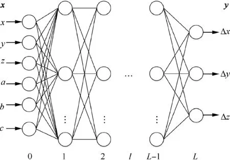
Fig.1 Schematic diagram of NN structure.

It is worth noting that the output of the input layer is equal to its input,namely

Inputting the data x into the NN,and computing it layer by layer according to Eq.(1),one can acquire the output of the network a.

Define the loss function as E(y，y)with ybeing the desired output of the NN,which is used to reflect the degree of inconsistency between the actual and desired output values.The NN is trained typically by error backpropagation (BP) algorithm,to continuously adjust the parameters Wand bof each layer neurons,through multiple forward and backward calculations aiming at minimizing the loss function.After each parameter update,the loss function value is recalculated to determine whether to continue to update the parameters or not.Upon using the desired pose and the actual error of the sampling points as the input and output of the NN,respectively,one can realize the error prediction by training the NN.

2.2.Genetic particle swarm optimization algorithm

The number of hidden layers and nodes has a significant influence on the performance and prediction accuracy of NNs.Generally,to ensure high enough generalization ability of the NN,and to avoid ‘‘over-fitting” phenomenon,a compact network structure should be selected as much as possible.Currently,there is still no effective theory to guide the selection for the optimal value of the number of hidden layers and nodes,which is mainly determined by empirical formulas.Besides,the initialization of the weights and the thresholds are also important to the convergence performance of NN algorithms.The random initialization methods commonly used can easily put the search range of the network parameters into the nonoptimal interval,causing the network to converge slowly.

A GPSO algorithm is proposed in this paper to obtain the optimal value of the number of hidden layer nodes,the number of hidden layers,the initial weights and thresholds for the NN,to finally realize the prediction of the robot’s positioning error.It adopts the selection and crossover operations in the genetic algorithm to generate a new population for expanding the search space of the particle swarm,and implementing the update.The position and speed of the particle swarm can be acquired as

where Xand X(=1,2)represent the positions of the child and parent particles respectively;Vand V(=1,2) represent the velocities of the child and parent particles respectively;is the crossover probability;the subscriptis the number of the child particles or the parent particles.

In this study,the particle positions are used to represent the number of the hidden layers and nodes,the initial weights and thresholds for the NN,and the mean square error (MSE)between the actual output and the desired output of the NN is selected as the fitness function

The training process of the NN model based on the GPSO algorithm is shown in Fig.2,which can be clarified as follows:

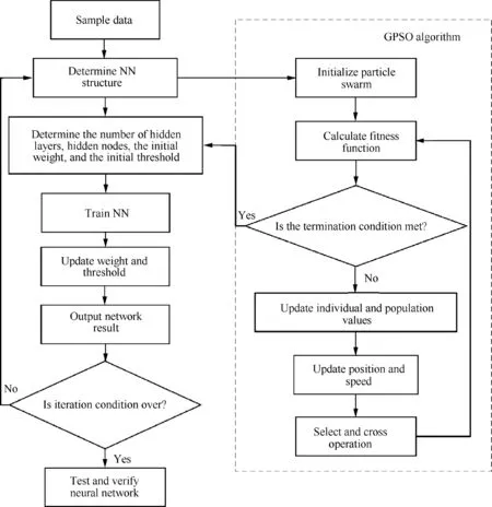
Fig.2 Flowchart of NN model training with GPSO algorithm.

(1) Normalize the sample data and divide them into training samples and test samples according to a certain proportion.

(2) Determine the range of the number of hidden layers and nodes,and initialize the network structure.

(3) Obtain the optimal parameters of the NN using the GPSO algorithm under the current network structure.

(4) Train the NN utilizing the BP algorithm,and test the network structure and the prediction results.

(5) Determine whether the loop condition of the algorithm is satisfied,if not,terminate the loop and store the most accurate network structure and the corresponding prediction results;otherwise,return to step (2).

The obtained NN model,i.e.,the prediction model of the robot’s positioning error,is then used to predict the positioning error of the robot’s target points.

2.3.Positioning error compensation

Based on the previous section,the error compensation strategy is presented in this section,which can realize the compensation of the robot’s positioning error without modifying its kinematic parameters.The basic principle is to correct the command pose of the robot by identifying its positioning error of the points to be compensated,then to make the robot move to the target position.The proposed approach is essentially an open-loop control method for the robot’s positioning accuracy before it executes the machining operation.The principle of the NN-based error compensation method for the robot is shown in Fig.3,and the associated process is as follows:

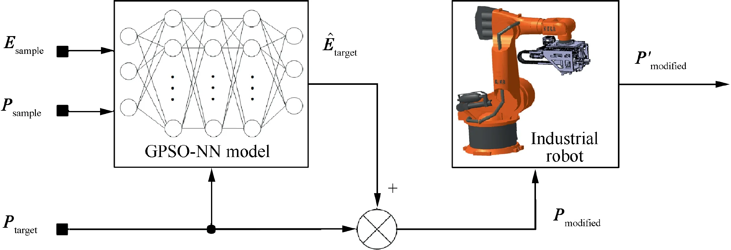
Fig.3 Schematic of error compensation based on NN.

(1) Select an appropriate sampling method to plan the robot’s task workspace,and obtain the desired pose Pof the corresponding sampling points.

(2) Measure the actual pose by a laser tracker,and calculate the positioning error Eof the sampling points.

(3) Train the NN model by taking Pand Eas the input and output,respectively,to acquire the prediction model of the robot’s positioning error.

(4) Input the desired pose of the points to be compensated Pinto the trained NN model,and output the predicted value of the robot’s positioning error ^E.

(5) Superimpose the predicted value ^Eon the desired value Pto obtain the corrected value P,i.e.,P=P+^E.

(6) Input the corrected command Pinto the robot’s control system to drive its movement,and the actual position of the robot is P,which is quite close to the desired value of the target point.

3.Training of neural network

3.1.Acquisition and processing of sample data

The KUKA KR 500-3 articulated robot is considered in this paper,as shown in Fig.4.The planning of sampling points is conducted in the robot’s Cartesian space.A laser tracker is adopted to measure the positioning error of the robot.To ensure that the sampling points can reflect the state of the entire working space of the robot as much as possible,the Latin Hypercube Sampling (LHS)method is used to plan the sampling.A rectangular parallelepiped area with a size of 600 mm×700 mm×1000 mm and an attitude angle of±15° is chosen as the sampling space,as shown in Fig.5.According to the LHS method,10 position coordinates and 30 attitude angles are randomly generated in the sampling space,and then they are arranged and combined to achieve the desired pose of 300 sampling points.The desired pose of the sampling points obtained by the above sampling plan is sent to the robot’s control system and the robot is controlled to move to the position of the instruction points in sequence,then the positioning error of the 300 sampling points is measured by the laser tracker.

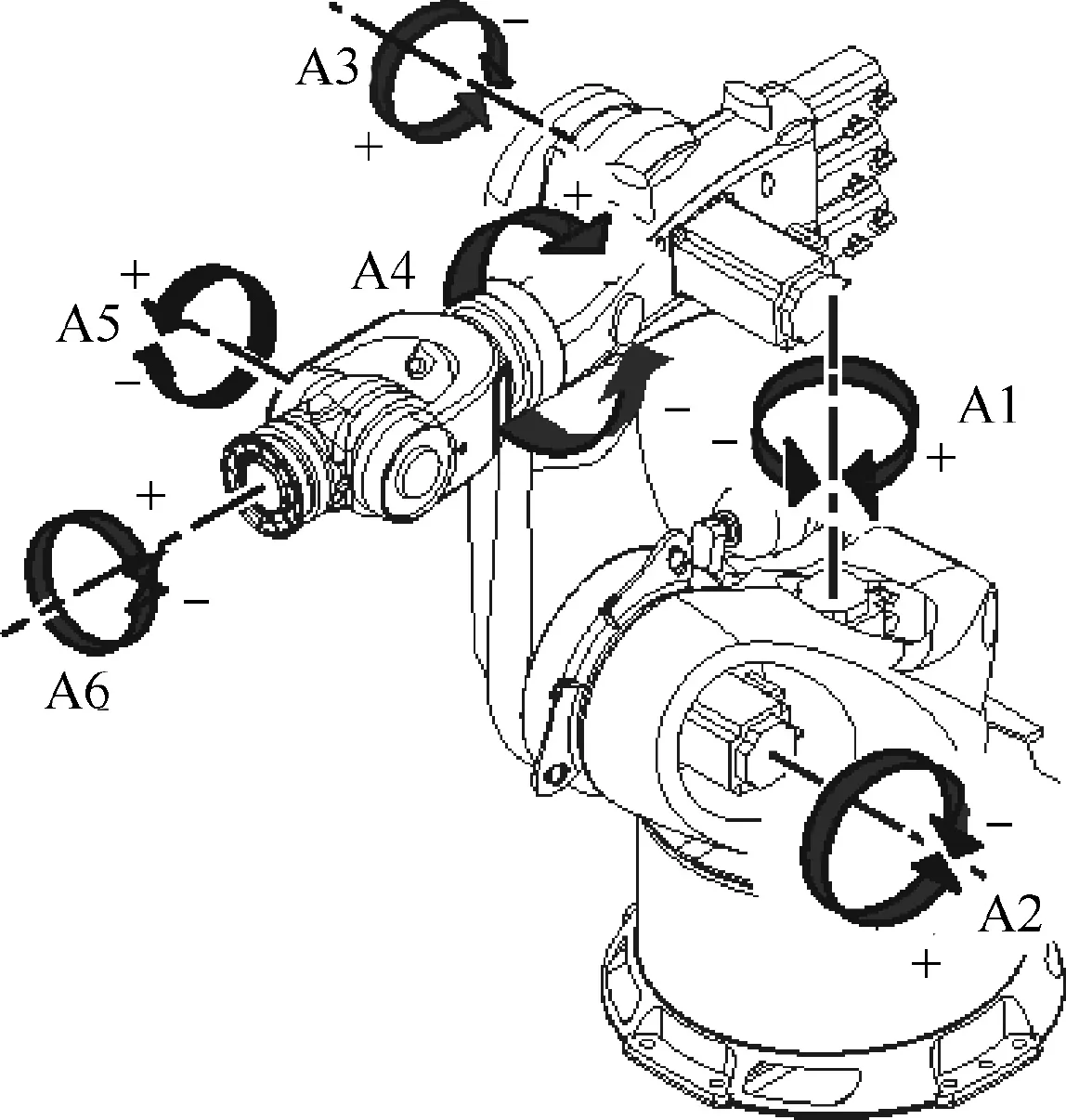
Fig.4 KUKA KR 500-3 articulated robot and its joint axis steering.25

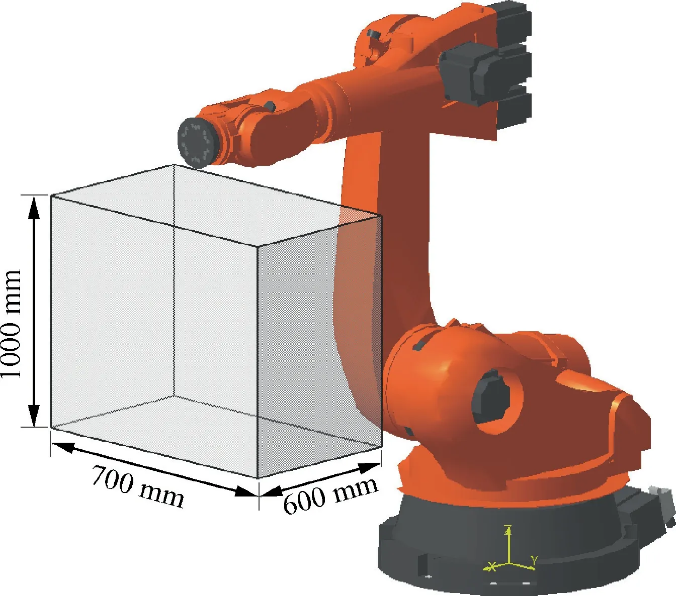
Fig.5 Schematic diagram of sampling range for robot’s Cartesian space.

The data collected typically need to be normalized for eliminating their dimensional difference.To ensure that the sample data can function and eliminate the difference between them,in this paper,the maximum normalization method is used.The transformation function is defined by

whereis the normalized data,the original data,the minimum value of the original data,andthe maximum value of the original data.

3.2.Training and prediction of neural network

The number of training samples is a critical factor in the NN.Therefore,it is necessary to study its influence on the NN prediction accuracy and determine the optimal range to ensure the accuracy and efficiency of the robot’s positioning error compensation.Firstly,according to the LHS method,2500 data of the desired pose in the workspace of KUKA KR 500-3 robot are produced as training samples.Assumed that the number of nodes in the hidden layer is.100,200,...,2400,2500 sets of samples are utilized,respectively,to train the NN for investigating the influence of the number of samples on the NN prediction deviation.Additionally,another 100 sets of sampling data are generated to test the prediction accuracy of the optimized NN model.Finally,the deviation between the predicted positioning error and the actual one is calculated.The maximum prediction deviation vs.the number of samples curve is shown in Fig.6(a),and in(b)is shown the average prediction deviation-the number of samples relationship.

From Fig.6(a),it is observed that when the number of samples is less than 2000,the maximum prediction deviation shows a downside with the increase in the number of samples;when it is larger than 2000,the maximum prediction deviation remains approximately unchanged.Besides,the maximum prediction deviation converges ultimately to 0.17 mm.It is obviously from Fig.6(b) that like the result of the maximum prediction deviation,the average prediction deviation shows a trend of falling first and then remaining constant as the number of samples improves.Moreover,when it exceeds 2000,the average deviation converges to nearly 0.08 mm.It can be concluded from the above analyses that when the number of samples is sufficient,the trained NN can reach a high prediction accuracy.

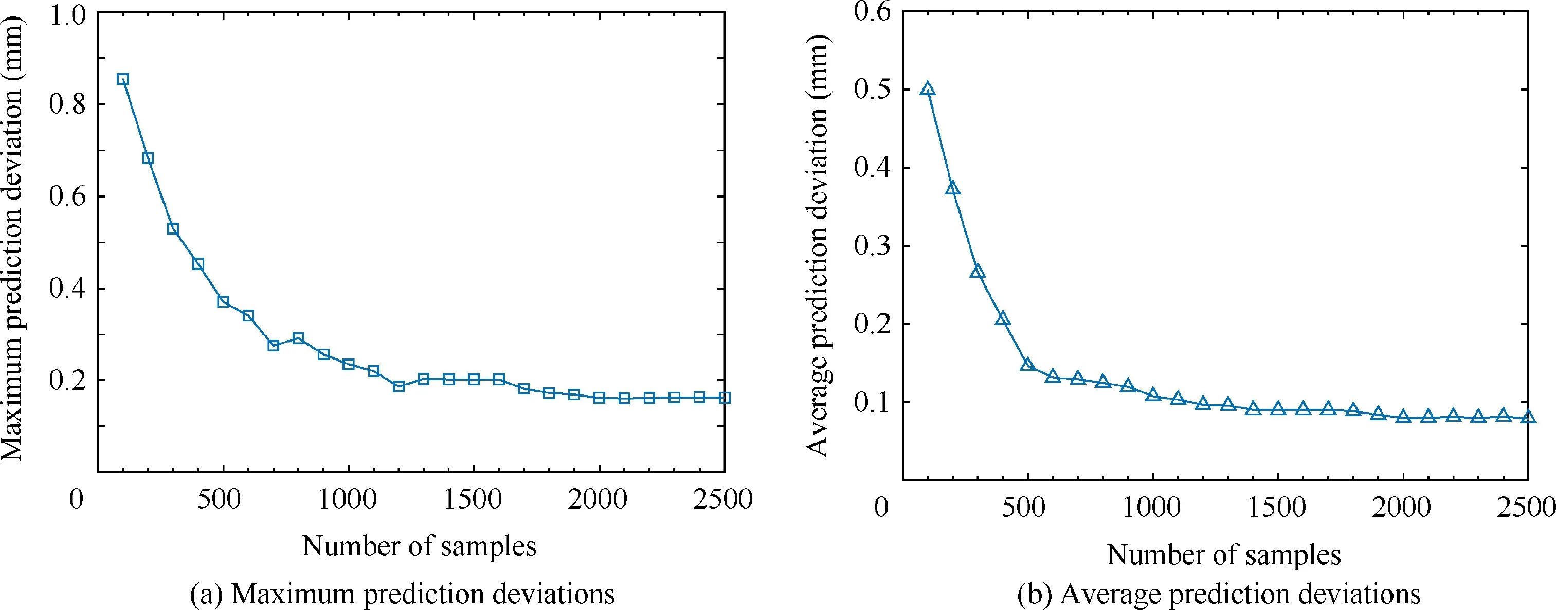
Fig.6 Prediction results vs.number of samples.

Because the measurement for the sampling data is the most time-consuming step in the robot’s error compensation process,to improve the efficiency,the number of training samples should be reduced as much as possible under the premise of ensuring the compensation accuracy.Based on the above research,the number of samples is selected as 1900 for the NN prediction in this paper.

According to the ratio of 19:1,the sample sizes in the training set and the test set are 1900 and 100,respectively.Some parameters of the NN model to be trained are tabulated in Table.1.The training of the NN is implemented based on the GPSO algorithm presented in Section 2.2,and the corresponding results are shown in Fig.7.Fig.7(a) shows the performance changes during the training of the NN model,which is evaluated using the MSE.It can be seen from Fig.7(a) that the MSEs of the model loss function corresponding to the training set,test set,and verification set decrease first and then stabilize as the number of training enlarges.The green circle in the figure indicates the best performance of the verification set,i.e.,the training accuracy of the verification set is the highest at the training times of 25.The MSE roughly converges to 10not reaching the target threshold of 10,which suggests that the NN model does not continue to converge after the training reaches a certain level.The relationship curve of the gradient vs.the number of iterations is shown in Fig.7(b).It can be found that with the increase of the training times,the gradient first decreases,then rises and finally converges to 0.006665 when the iteration reaches 31.

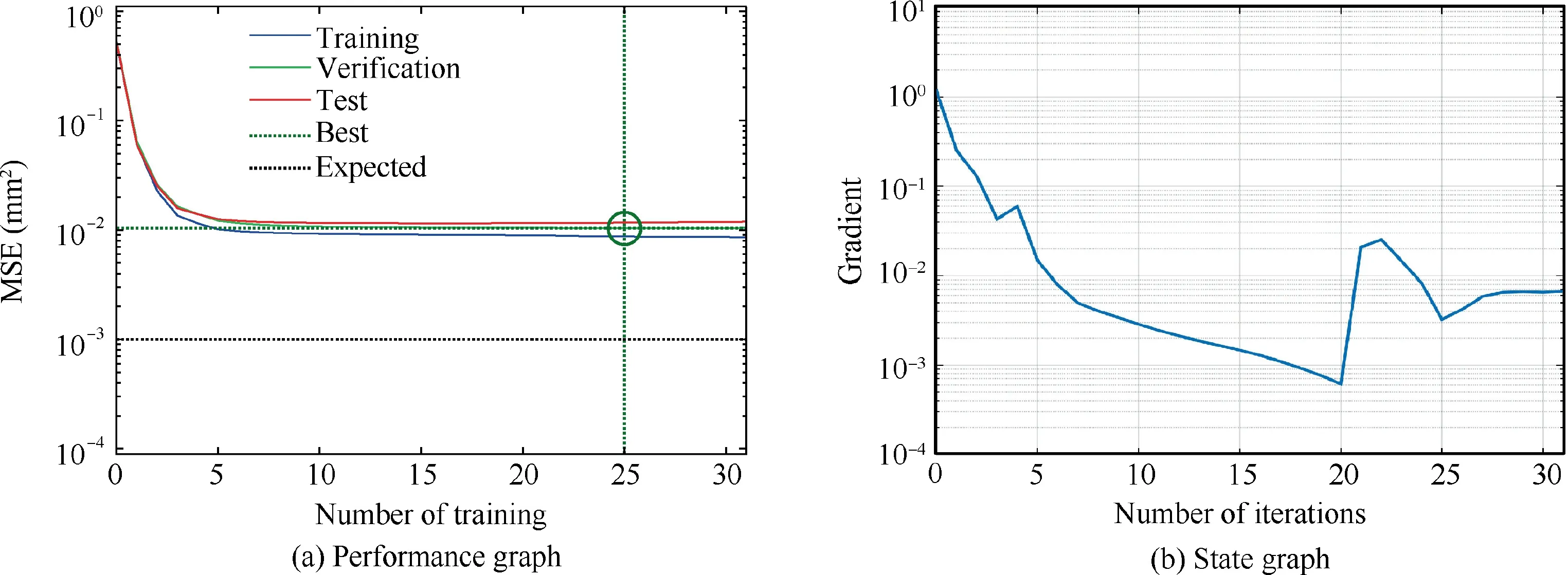
Fig.7 Training results of NN.

The regression line,shown in Fig.8,is obtained to measure the degree of fit of the trained NN corresponding to the data set.It can be observed form Fig.8 that the model regression correlation coefficients associated with the training set,the verification set,the test set and all the samples are=0.95881,=0.95302,=0.94521 and=0.95591,respectively.All the four regression coefficient values approach 1,which means that the trained NN fits the sample data to a high degree with a satisfactory regression performance.

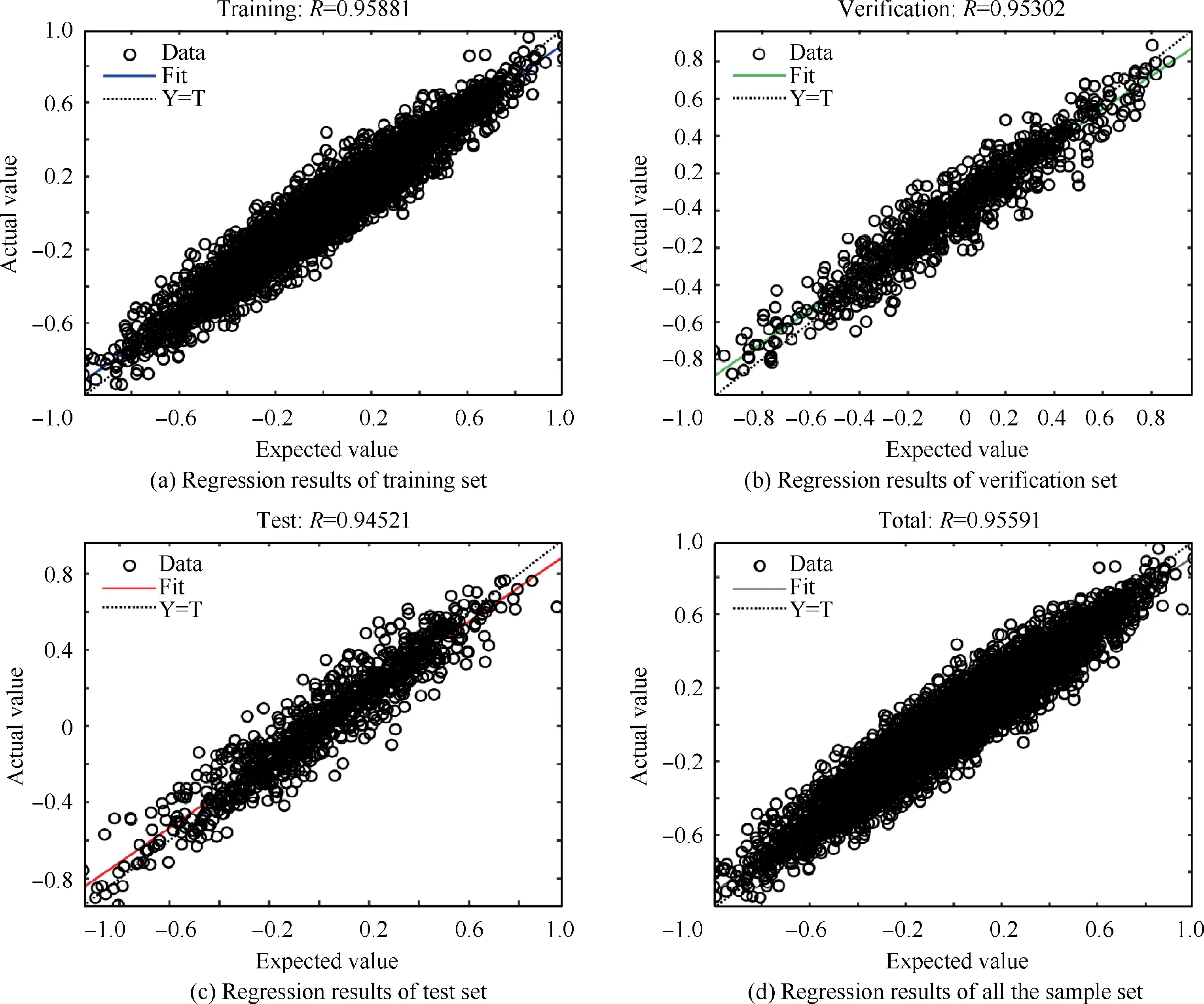
Fig.8 Regression performance results of NN.

Then the trained NN is utilized to predict the positioning error of 100 points in the test set.The model prediction deviation with the highest accuracy is shown in Fig.9,which is obtained by comparing the predicted errors with the actual ones.From Fig.9,the prediction deviation is within 0.25 mm,which indicates that the prediction accuracy of the NN model is acceptable.The results of the obtained NN are shown in Table.2,from which it can be seen that the number of the hidden layers is 3 with the numbers of nodes of 15,10,and 5,respectively.Furthermore,the MSE of the training set is 0.00859,which suggests that the optimized model is well-fitted for the training set.The training time is 3 s,showing that the model training efficiency is high.Besides,the accuracy of the test set is 83.33%,which manifests that the trained NN has a high accuracy in predicting the robot’s positioning error.

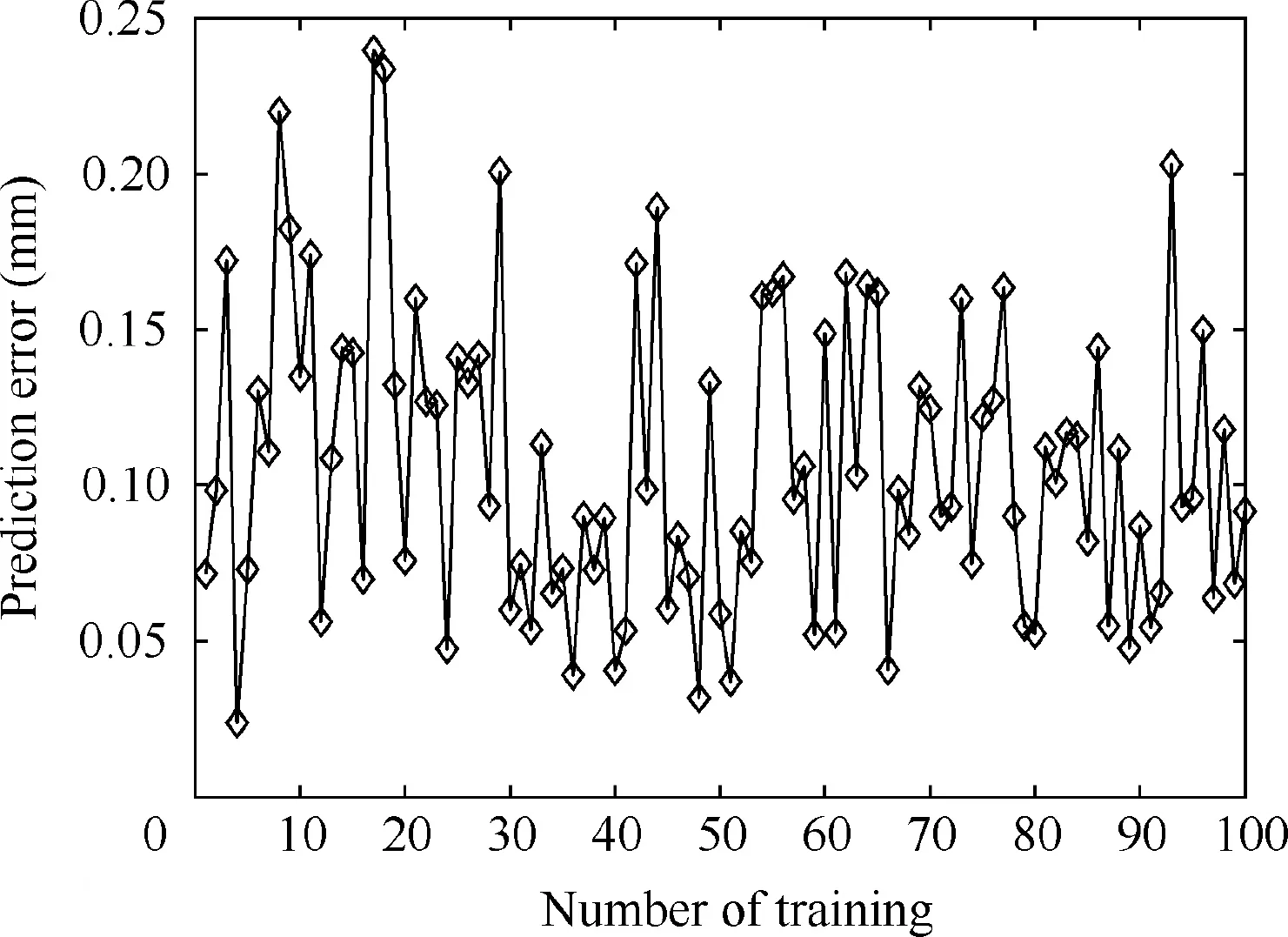
Fig.9 Model prediction deviation.

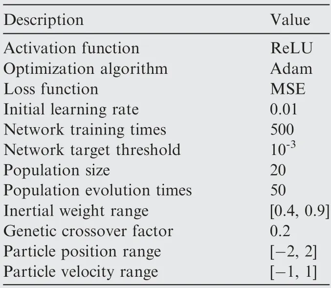
Table 1 Some parameters of NN model.

Table 2 Results of obtained NN.

4.Experimental verification

4.1.Experimental platform

The experimental platform is developed strictly for the purposes of conducting the current research,and is illustrated in Fig.10.It consists of the KUKA KR 500-3 industrial robot with an end effector,the API Radian laser tracker with target ball and other equipment.Partial performance parameters of the robot are shown in Table.3.The end effector is a drilling spindle,which is mounted on the flange of the robot to realize the machining.The API Radian laser tracker is adopted as the sensor,which can track a moving point in space statically or dynamically,and determine its spatial coordinates.Its main parametric specifications are shown in Table 4.Two scenarios of no-load and drilling are carried out to validate the GPSONN approach proposed in this paper.

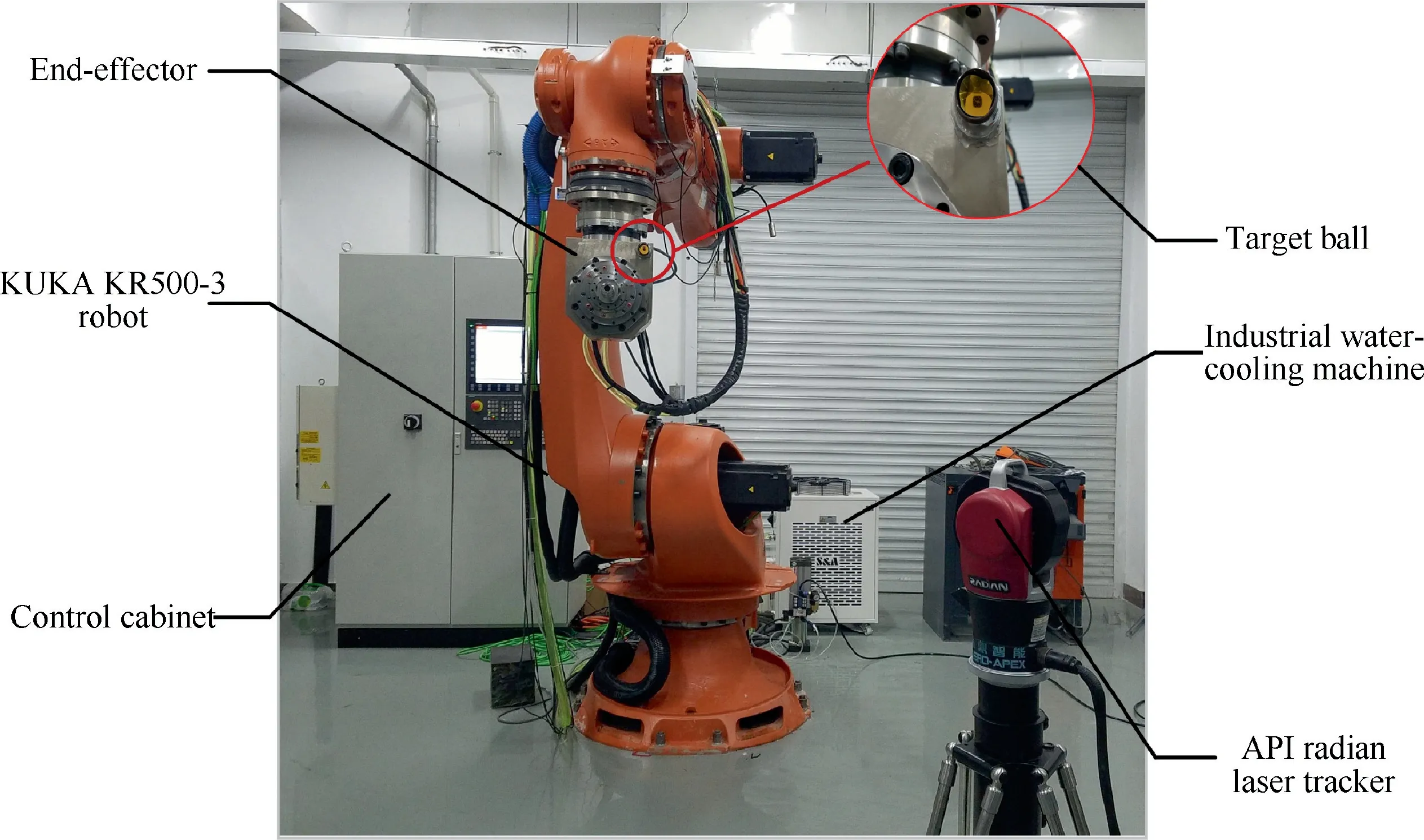
Fig.10 Experimental platform.

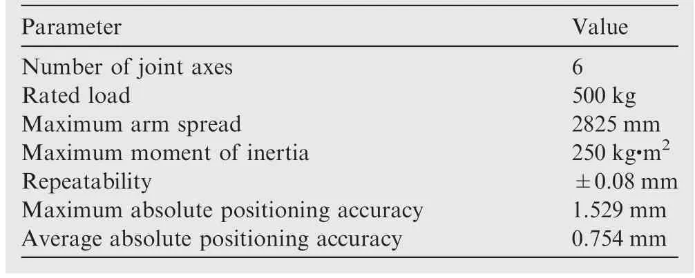
Table 3 Basic parameters of KUKA KR 500-3 robot.

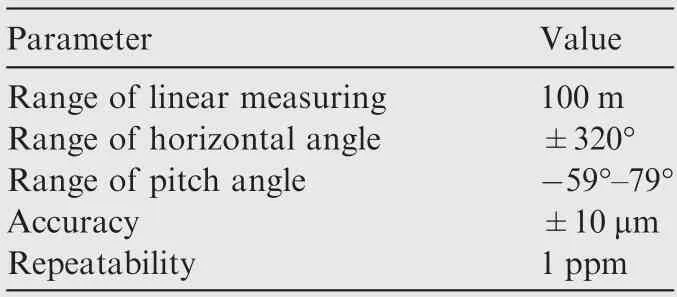
Table 4 Specifications of API radian laser tracker.

4.2.No-load scenario

Firstly,the proposed approach is individually applied to the robot in the no-load scenario.For comparison,the other methods are then used to compensate for the robot’s positioning error.

The experimental procedure in this paper is as follows:

(1) Plan a cuboid area with a size of 600 mm×1200 mm×800 mm and with an angle range of a ∈[-10，10],b ∈[-10，0],and c ∈[-10，10]in the robot’s workspace;then generate randomly 2000 sampling data using the LHS method.

(2) Input the above-mentioned sampling points into the robot’s control system and actuate it to the command points sequentially.Meanwhile,measure the actual position coordinates of the command points via the laser tracker,and compute the errors by comparing them with the desired position coordinates.

(3) Divide the positioning errors of 2000 sampling points into the training and test sets in terms of the ratio of 19:1 to train the NN model,and input the desired pose of the verification points into the trained NN to predict the robot’s positioning error.

(4) Correct the position coordinates of the verification point according to the predicted result in step (3);enter the corrected points into the robot and utilize the laser tracker to measure their actual position coordinates;then compare them with the desired values to obtain the positioning errors of the compensated points.

From Fig.11(a)-(c),it is obvious that the positioning error of the robot in each direction before compensation exceeds 0.8 mm,which cannot meet the accuracy requirement of 0.5 mm for aircraft assembly.Particularly,the positioning error in theaxis generally deviates to the negative direction,while the positioning errors in theandaxes deviate to the positive direction,and none of them fluctuate around 0 mm.The reason is that on the one hand,the robot’s various error sources have different effects on the positioning accuracy in,andaxes,on the other hand,in the process of establishing coordinate system,error transmission and accumulation have a deviation on the positioning accuracy of all directions,resulting in different error distributions in,andaxes.Moreover,it can be found from Table.5 and Fig.11(a)-(c) that the positioning error of the robot inaxis reduces to within 0.35 mm,and the positioning errors in theandaxes decline to within 0.2 mm after compensation.Besides,the error fluctuation range in each direction with compensation becomes smaller compared to that without compensation.From Table.5,the maximum total error of the robot is reduced from 1.529 mm to 0.343 mm,and the average error is decreased from 0.754 mm to 0.223 mm,i.e.,the maximum positioning error and average error of the robot are reduced by 77.57% and 70.42%,respectively.The above analyses prove the effectiveness of the error compensation method based on the NN proposed in this paper.

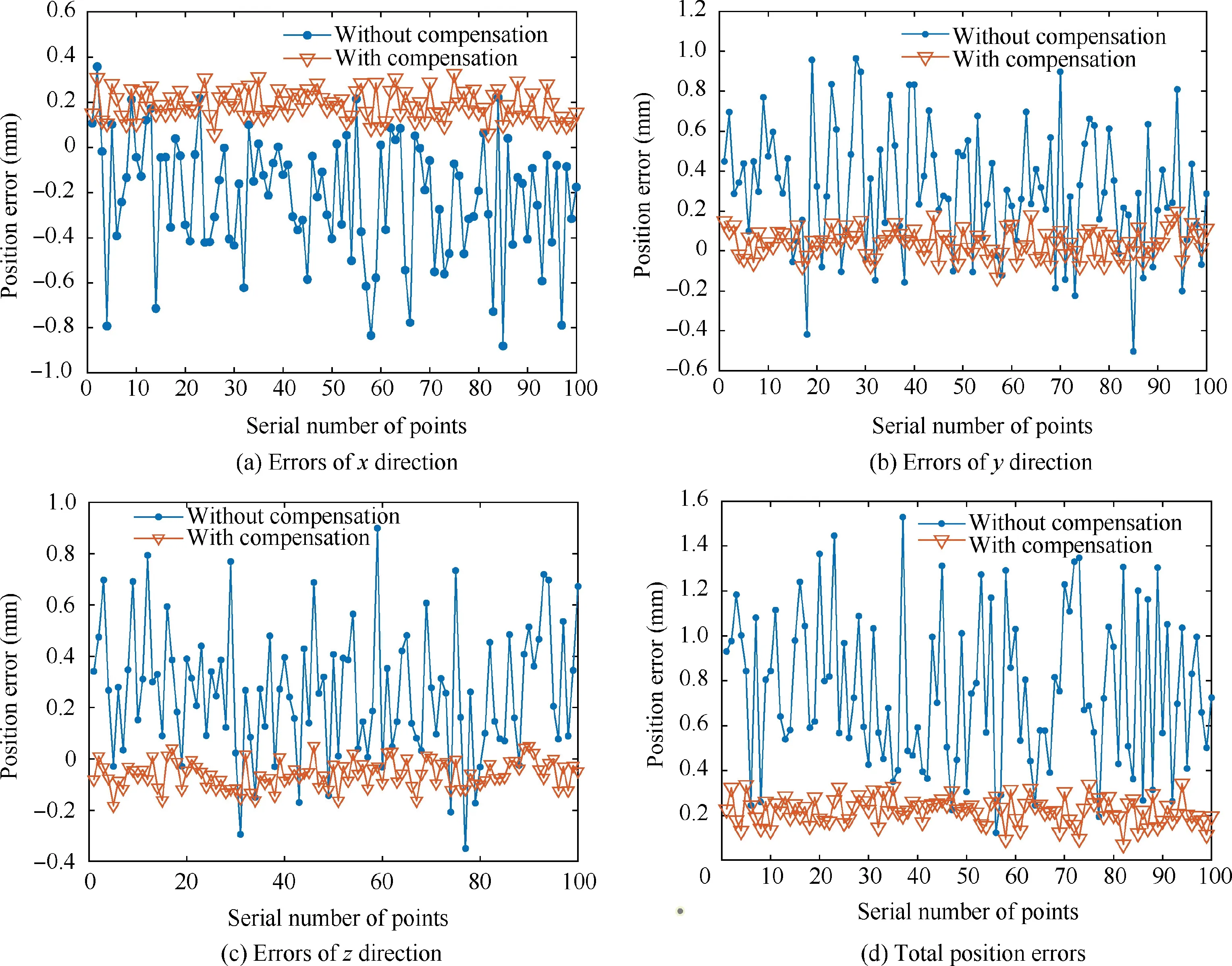
Fig.11 Position errors without and with proposed method under no-load scenario.

Table 5 Statistics of positioning error with and without compensation.

The proposed GPSO-NN method in this paper is compared with ELM,parameter identification,and traditional neural network(TNN).The data statistics of the total error with and without compensation of these methods are shown in Table 6.To show the experimental comparison results more intuitively and clearly,the contrast line chart and the frequency histogram are shown in Fig.12.By analyzing the experimental results in Table 6 and Fig.12,it is clear that the total error after compensation for each method is significantly lower than that before compensation.All the compensated errors are reduced to within 0.5 mm,which shows that these methods have effectiveness and feasibility for the robot’s accuracy enhancement.Additionally,from Fig.12(b),it can be seen that the errors compensated with the proposed method almost fall within the interval of 0.1-0.3 mm,while most of the errors compensated by the other methods are within the interval of 0.2-0.4 mm,which shows that the proposed method has the best effect for error compensation of the robot.Furthermore,it can be found that the maximum total error of the proposed method is 0.343 mm,smaller than 0.503 mm,0.474 mm and 0.453 mm of the other three methods after compensation.In summary,the comparative results demonstrate that the error compensation method based on GPSO-NN proposed in this paper can effectively improve the positioning accuracy of the robot.Compared with the other three error compensation approaches,the proposed method has the lowest compensation error for the robot,which proves the accuracy and superiority of this method.

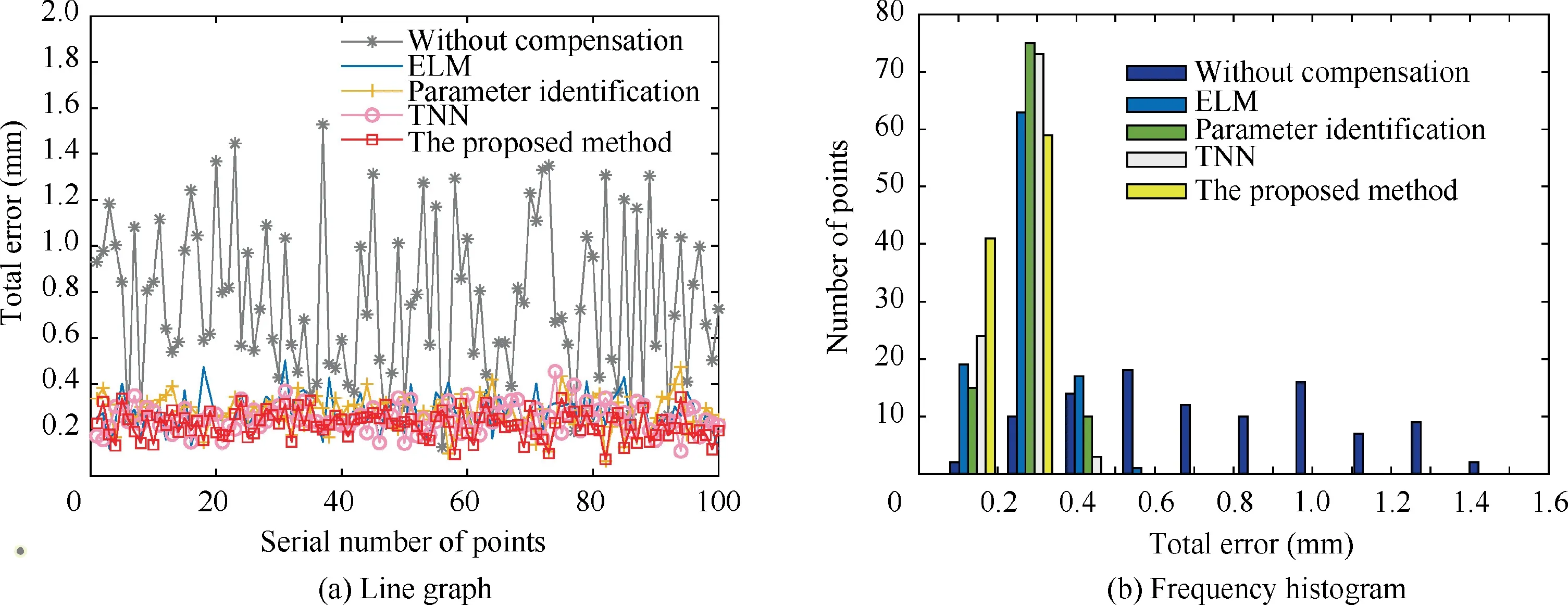
Fig.12 Comparison of total positioning error without and with compensation.

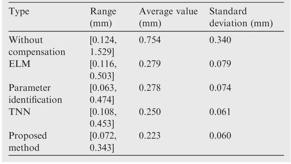
Table 6 Comparative results of total error for robot.

4.3.Drilling scenario

The error compensation method proposed in this paper is for the operation of robotic drilling in aircraft assembly.Therefore,it is necessary through the drilling experiment to verify whether the positioning accuracy by this method can meet the accuracy requirements.In the experiment,the tool coordinate system{T}and the product coordinate system{P}are the two most important frames for performing the drilling operation.The device shown in Fig.13 is used to establish the tool coordinate system {T},where the auxiliary measuring rod is clamped on the motorized spindle,and the target ball of the laser tracker is fixed on the target holder at the end of the measuring rod.The center point of the target ball is the origin of the tool coordinate system {T};the-axis is the spindle feed direction;the-axis is along the-axis of the robot’s base coordinate system;the-axis is determined by the right-hand rule.The product is fixedly installed on the tooling,and the establishment of the product coordinate system {P} generally requires drilling some reference holes in advance.Two reference holes are pre-drilled in a relatively flat plate to build the product coordinate system {P},as shown in Fig.14.Theaxis is the direction of the straight line formed by reference holes 1 and 2;the origin is the center of the circle for the reference hole 1;the-axis is the straight line perpendicular to the plane of the product;the-axis is determined by the right-hand rule.

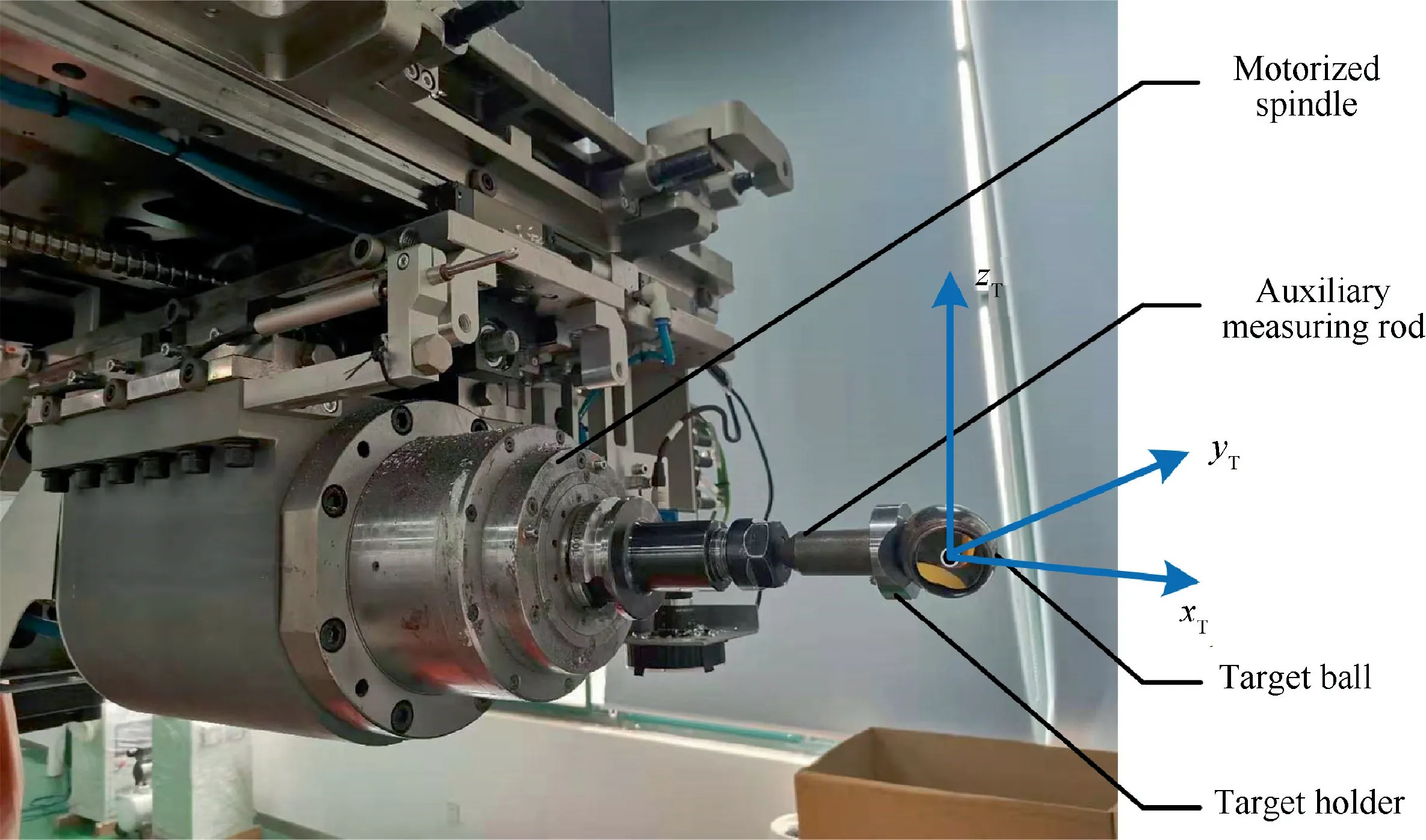
Fig.13 Tool coordinate system and installation of target ball of laser tracker.

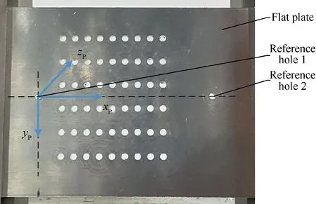
Fig.14 Schematic diagram of product coordinate system.

The scene of the robotic drilling is shown in Fig.15.The workpiece is mounted on the tooling through the fixture,and 54 positions to be drilled are planned in the product coordinate system {P}.The-direction hole spacing is 8 mm,and thedirection hole spacing is 15 mm.The robot with and without compensation is actuated respectively to drill holes;finally,a three-coordinate measuring instrument is utilized to measure the positioning error of the drilled holes.It is worthwhile noticing that in the drilling experiment,the end-effector of the robot is composed of a drilling tool driven by a motorized spindle and a pressure foot driven by a feed motor,shown in Fig.16.In the end-effector,a length gauge is mounted on the motorized spindle.Before drilling,the pressure foot is pressed directly to the workpiece’s machining plane with a desired force,then the feed spindle starts drilling depending on the measurement from the length gauge to ensure the holedepth.Particularly,the depth of the hole drilled by the robot is the difference between the measured value and the preset value of the length gauge,and is almost unaffected by the-direction error of the robot.Hence,synthesizing the cost,the complexity and the accuracy,the-direction error of the robot is not considered in our drilling experiments.To prove the abovementioned point of view,four groups of comparative experiments,where the holes with a depth of 12 mm are drilled,are conducted to assess the positioning accuracy of the drilled holes.

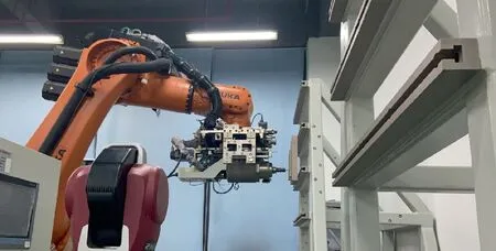
Fig.15 Scene of robotic drilling.

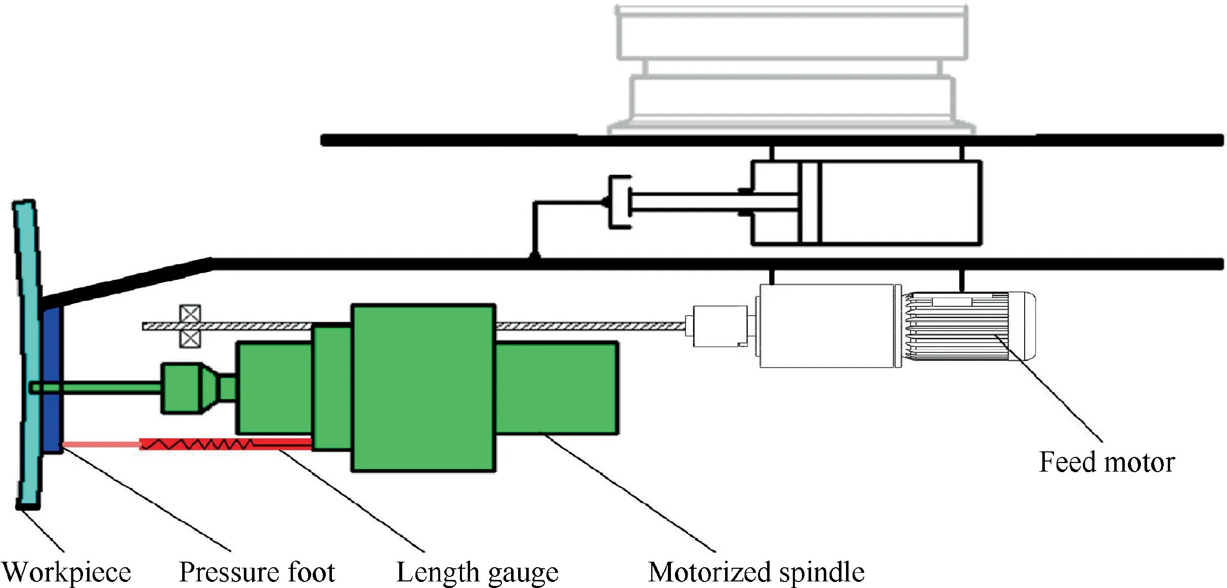
Fig.16 Robot’s end-effector with pressure foot and length gauge.

Group 1:without compensation and without length gauge.

Group 2:with compensation and without length gauge.

Group 3:with compensation and with length gauge.

Group 4:without compensation and with length gauge.

Table 8 Statistics of positioning error of drilled holes.

Table 7 Key process parameters related to robotic drilling.

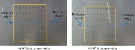
Fig.17 Drilling Robotic drilling results.

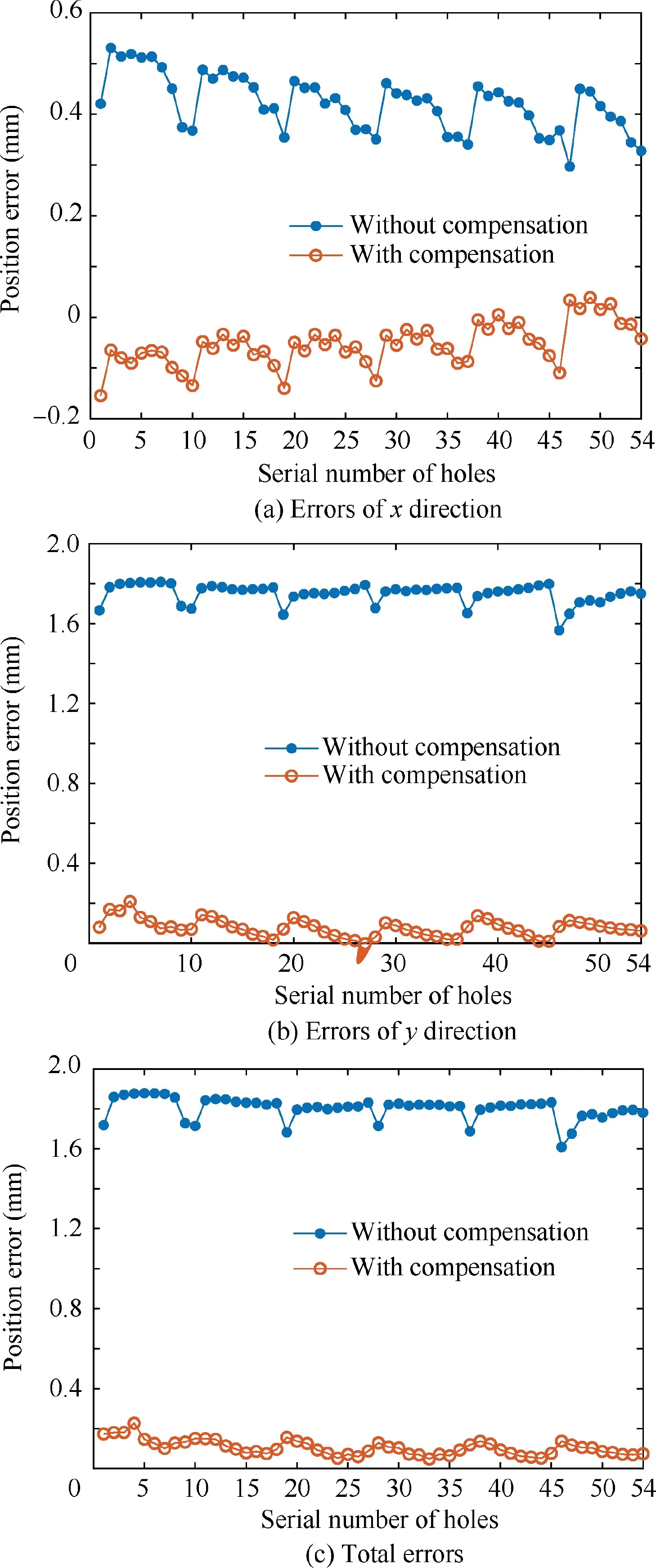
Fig.18 Position errors of drilled holes with and without compensation.

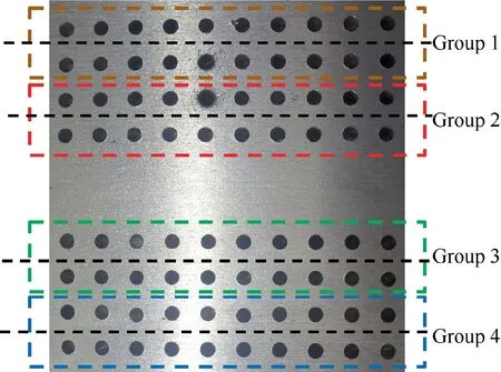
Fig.19 Results of robotic drilling under different conditions.

The comparative drilling results are shown in Figs.19 and 20.From Fig.20,it can be seen that the positional errors of the holes in theanddirections show great variability for the compensated and uncompensated robot.It means that the accuracy of the robot itself affects significantly the positional error of the holes in theanddirections.In addition,the error of the holes in thedirection is an order of magnitude smaller than the errors in theanddirections for all the four groups of drilling experiments.Furthermore,it can be observed that thedirection error of the holes exhibits a slight difference for both the compensated and uncompensated cases with length gauge,which indicates that it is whether to use the length gauge as a feedback that exerts a profound influence on thedirection error of the holes.Hence,the-direction errors of the holes for all the drilling experiments in this paper are guaranteed by the length gauge,regardless of the-direction accuracy of the robot.

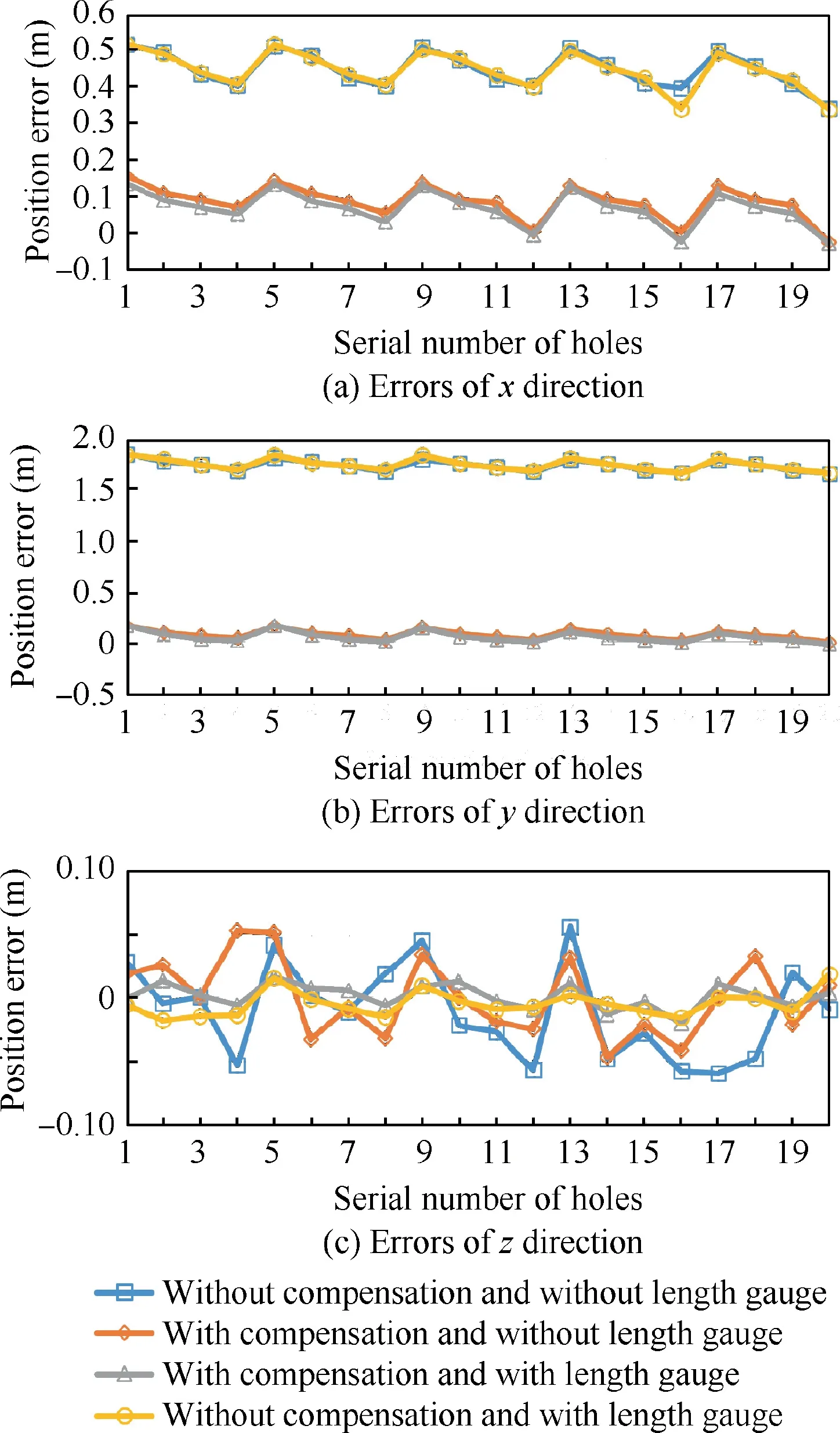
Fig.20 Position errors of drilled holes under different conditions.

5.Conclusions

An accuracy enhancement method of an industrial robot based on the GPSO-NN is proposed in this paper.A NN is constructed to predict the positioning error of the industrial robot using the GPSO algorithm.Furthermore,the error compensation is realized for the KUKA KR 500-3 industrial robot.The experimental results show that the proposed method can reduce the positioning error from 1.879 mm to 0.227 mm,increasing the drilling accuracy of the robot by 87.9%.The above results verify the effectiveness and feasibility of the proposed method in terms of reducing the robot’s positioning error.

The proposed method in this paper can only improve the robot’s position accuracy.Future study can be focused on expanding the method to the error compensation of the robot’s posture.In addition,the transfer learning can be further studied to extent directly the trained NN of the KUKA KR 500-3 robot to other types of robots for the purposes of error compensation.

The authors declare that they have no known competing financial interests or personal relationships that could have appeared to influence the work reported in this paper.

This study was co-supported by the Natural Science Foundation of Jiangsu Province(No.BK20190417),the National Natural Science Foundation of China (No.52005254) and the National Key R&D Program of China (No.2018YFB1306800).