A combined technique of Kalman filter, artificial neural network and fuzzy logic for gas turbines and signal fault isolation

Simone TOGNI, Theoklis NIKOLAIDIS, Suresh SAMPATH

Department of Power and Propulsion, Cranfield University, Cranfield MK-43, United Kingdom

KEYWORDS Artificial neural network;Data analytics;Data filtering;Diagnostics;Fuzzy logic;Gas turbine;Kalman filter;Performance-based diagnostics

Abstract The target of this paper is the performance-based diagnostics of a gas turbine for the automated early detection of components malfunctions. The paper proposes a new combination of multiple methodologies for the performance-based diagnostics of single and multiple failures on a two-spool engine. The aim of this technique is to combine the strength of each methodology and provide a high success rate for single and multiple failures with the presence of measurement malfunctions. A combination of KF (Kalman Filter), ANN (Artificial Neural Network) and FL(Fuzzy Logic)is used in this research in order to improve the success rate,to increase the flexibility and the number of failures detected and to combine the strength of multiple methods to have a more robust solution.The Kalman filter has in his strength the measurement noise treatment,the artificial neural network the simulation and prediction of reference and deteriorated performance profile and the fuzzy logic the categorization flexibility,which is used to quantify and classify the failures.In the area of GT(Gas Turbine)diagnostics,the multiple failures in combination with measurement issues and the utilization of multiple methods for a 2-spool industrial gas turbine engine has not been investigated extensively.

1. Introduction

The performance-based gas path analysis is a topic that has been studied in the last 40 years since Urban1defined the possibility of making diagnostics on the gas turbines components,based on the performance parameters. The other consolidated techniques that had taken place before,were the vibration and the lube oil diagnostics.The first consists of checking the bearing absolute and relative vibration caused by unbalance,rotor bow,rotor crack or blade separation and the second of checking if debris,caused for example by erosion,are present in the lubrication oil circuit. These techniques, especially the vibration diagnostics, are renowned for malfunction detection and for prognostics. Instead, the performance-based diagnostics proposes to detect loss of performances and malfunctions from the early stages of operation with several clear advantages:identifying which part of the engine is subjected to shortages,evaluate different schedules for a certain engine to save its lifetime or reduce maintenance costs, prevent unplanned outages,extend the lifetime of certain components.Indeed,the maintenance costs on industrial gas turbines and combined cycle plants can reach 50%of the total O&M(Operation and Mainteinance) costs2that represent 7% of the overall project cash flow. Additionally, statistic studies conducted over 3000 E and F class engines concluded that the unplanned maintenance cost can reach 8% of the O&M costs, or 2% of net revenue income and the loss of revenue can reach the 15% of the O&M cost or 5% of net revenue income.3

A methodology is intended to offer an easy way to detect the components deterioration or failure.4The final set up for the health monitoring should include the features remarked by the experts in this field:5interface with the increasing amount of data available from the engines; integrate new sensor suites and capabilities; precise modelling of the baseload and part load conditions; leverage all available information including user-specific inputs; have a practical design. What is meant to be detected is the deterioration of every single component – single failure – and the combination of components deterioration – multiple failures. The measurements bias are omitted since, due to the redundant measurements available in the industrial gas turbines,have fewer chances to be encountered. This assumption is also supported by Kerr et al.6Measurements noise instead,shall also be part of the simulation as they are relevant in any working engine. For instance, the detection of the multiple failures in combination with the detection of measurement noise is a point that has not been fully investigated in the reference.

Sampath and Singh7described how to detect multiple failures including measurements noise and bias.The methodology was built with an auto-associative neural network used to isolate the bias and a combined genetic algorithm,artificial neural network, employed to detect multiple failures. However, the methodology resulted in unsuitable for the online diagnostics.

Instead, multiple failures with single or the combination of multiple techniques have been frequently investigated in the references.Viharos and Kis8proposed a comparison of different neuro-fuzzy solutions. The authors found that the combination of the neural network learning, together with the fuzzy logic, reduces the setup time and improves the quality of the detection. In addition to that, fuzzy logic can be manually implemented to include some user-based rules.Wang et al.9introduced a series of fuzzy logic, which is coupled with the TOPSIS (Technique for Order of Preference by Similarity to Ideal Solution) methodology. Dewallef et al.10proposed a combination of Bayesian belief with Kalman filter in order to benefit from their mutual advantages. The Kalman filter is used to improve the information the Bayesian belief is using for the prediction of the failure. Verma et al.11instead, proposed a genetic fuzzy logic with a radial basis function neural network.The aim of the genetic fuzzy is to automatically tune the failures based on genetic algorithm analysis while the neural network is used to isolate the noise. The methodology is only tested for a single deterioration case scenario. Kumar et al.12coupled the fuzzy logic with the support vector machine not only for the diagnostics but also for the remaining lifetime estimation. Recent papers, taking advantage of the increasing knowledge and power of the neural network13applied it to the diagnostics of a gas turbine.Finally, Li et al.14coupled neural network with support vector machine for the quantification and classification of the gas turbine failures with standard white noise.

Comparing the reference review against the objectives stated at the beginning of the chapter, it can be seen that there’s no clear answer on the multiple failure detection together measurement noise.This is a primary objective to effort,as all the turbomachines will encounter both problems at the same time.

In addition to that, the growing computational capabilities increased the number of resources that can be employed in the performance-based diagnostics. The ANN (Artificial Neural Network), in particular, became faster and reliable both for fault isolation,noise reduction and for performance modelling prediction. It is a common point, among the papers coupling multiple techniques, the idea of taking the strength of each contributor while reducing their limitations. This can lead to a more robust combination.

Starting from these objectives of detecting multiple failures in combination with measurement issues and coupling the strength of multiple techniques a methodology has been built.The structure is thought in three phases:

(1) The data analytics, where the measurements are corrected by measurement noise.

(2) The key performance parameter prediction starting from the measurements previously corrected.

(3) The failure diagnostics in terms of quantification and classification of single and multiple failures.

For each phase,a contributor has been selected resulting in the combination of KF+ANN+FL.The Kalman filter has been selected for the measurement noise correction because of its performance and simplicity. In fact, as it is conceived to work with a big amount of data and with online signals, it has to be robust, fast and adaptable. The Kalman filter has been successfully used by Lu et al.15to improve performance monitoring.

Looking at the second step, the quantification of multiple failures needs to consider not only the measurement values but also the gas path parameters (efficiencies). The dedicated model needs to be accurate in order to calculate these parameters and its relationship16,17and the ANN has been successfully tested by Fast18and Kanelopoulos19et al.Moreover, in the light of increasing of the amount of available data, the ANN has been tested to be the right model to provide an enhanced understanding of the relationship between signal and failure, so far not deeply known or difficult to detect.20

The preferred method to perform quantification and classification of the failure is the fuzzy logic. This technique offers the possibility of clearly and easily quantifying the failures and it’s not much affected by the noise. Moreover, it is flexible enough to be used for quantification purposes or for classification reasons. Additionally, its adaptability allows increasing the number of rules, while detecting engine specific failures or while increasing the generic failure portfolio.Finally, the quantification done within the fuzzy logic frame offers the possibility to be used for prognostics purposes.12The fuzzy logic has been already tested by Eustace21and Palade et al.22

This combination is investigated in this paper and the objective is to offer a performance-based diagnostics, which is able to detect, with a high degree of confidence, both single and multiple failures with the presence of measurement noise.

2. Problem formulation

From the introduction,it is meant that the topic is intended to be investigated is the multiple failure diagnostics with the presence of measurements noise.The targeted type of failures considered is the compressor fouling, the turbine fouling and the turbine erosion, failing with different magnitude Refs. 23–32 The methodology that has been established for this purpose is divided into three sections (see Fig. 1):

(1) Data filtering to correct for noise.

(2) GT thermodynamic parameters prediction.

(3) GT components single and multiple failure quantification and classification.

Considering that no real data are available for the validation of the methodology, an additional step has been added at the beginning of the structure and is: GT Performance reference cycle modelling.

The research is focusing on the study of a new combination of multiple methodologies consisting of ANN, KF, FL.

The key contributors and their interaction are shown in Fig. 1. Where X are the measurements, n is the noise, nris the remaining noise, Δƞ and ΔX are the delta efficiency and measurement, Amb are the ambient conditions and ref is the reference of the non-deteriorated engine.

2.1. Performance modelling

The gas turbine considered is a 2-spool industrial gas turbine of small size with a pressure ratio of 17:1. The gas turbine has been modelled with hardware including two compressors and two turbines (Low Pressure Compressor (LPC), High Pressure Compressor (HPC), High Pressure Turbine (HPT)and Low Pressure Turbine (LPT)) in Fig. 2.

The performance values are modelled on Turbomatch the thermodynamic cycle modeller built and maintained at Cranfield University. Turbomatch is a software-based Gas Turbine performance simulation tool developed by the Propulsion Engineering Centre (formerly department of Power and Propulsion), at Cranfield University.32The tool is a 0-D performance simulation code, featuring off design and transient simulation as well Ref. 33.

The gas turbine is modelled to match the performance of 11.9 MWe with the pressure ratio of 17:1, an inlet mass flow of 41.6 kg/s and an exhaust temperature of 485°C. This is defined as the nominal condition. On top of it, the deterioration of one or multiple components is simulated (see Table 1).

The deterioration is built taking into account the relationship reported in the literature to make the simulation realistic.Based on the Refs.23–32,the ratio of delta efficiency(Δƞ)and delta air inlet mass flow (Δ) deterioration is set to 1:2.

2.2. Kalman filter

The Kalman filter is built to compensate for measurement noise. It relies on the MM (Multiple Measurements) installed on the industrial gas turbines. The number of probes used for each measurement point is five.33,34Exceptions are on the TET T6 where the probes increase to 1835and on the power P and fuel mass flowfuel, where the probes decrease to 1.The noise injected is randomly normally distributed around the mean value.Each probe is noised separately to have different values for each sensor.Moreover,as reported by Joly et al.36the level of noise of the pressure probes,is¼of the noise of the temperature probes. This relation is also applied, and the resulting reference 0.4% noise is shown in Table 2. The measurements bias,as already reported in Introduction are omitted since, due to the redundant measurements available in the industrial gas turbines, have fewer chances to be encountered.This assumption is also supported by Kerr et al.6

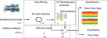
Fig. 1 Flowsheet of established methodology.

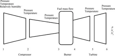
Fig. 2 Gas turbine measurements location.

Table 1 Efficiency vs mass flow for different types of failure.

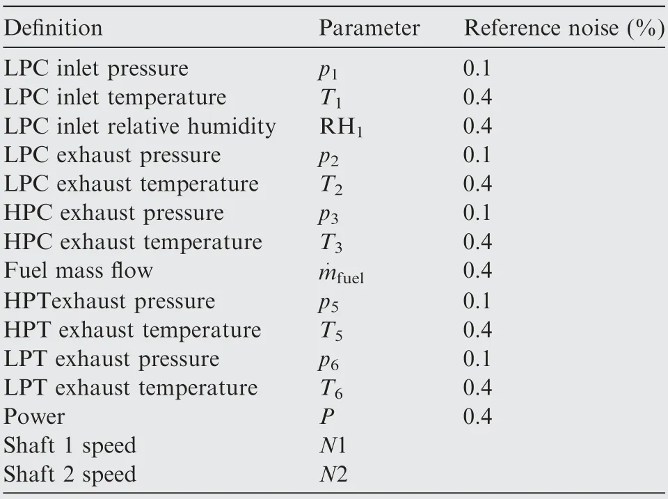
Table 2 Noise level.

The intent of the Kalman filter is to use all the available singles to make an information fusion at each point of the gas turbine (see Fig. 2) as already tested by Anitha37and Gu¨len35et al. In this way, the prediction is expanded by the number of measurements located at each measurement point and results on being more accurate. To apply this procedure two different types of structures have been built: a multiple-layer linear Kalman filter, Fig. 3 (The dashed lines show the measurement that is used as initial estimation (xk–)– Meas 1, Meas 3 and Meas 5 in the first layer,xk1in the second layer.),and a SLKF (Single Layer Kalman Filter), Fig. 4. With the MLKF(Multiple Layer Kalman Filter), the data are processed in two different layers before calculating the final output.Instead in the single-layer Kalman filter, the data are processed in a unique layer and fused to a single output.These two structures provide the opportunity to compare the additional expansion of information offered by the multiple layer configuration and the possible smearing effect associated with it. In fact, if it’s true that more layers can improve the prediction quality,it is also true that they can extend the measurements errors.

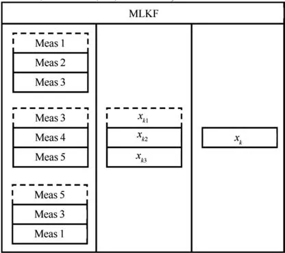
Fig. 3 Multiple layer linear Kalman filter set up.

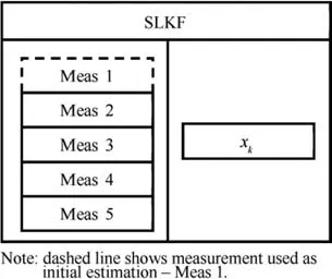
Fig. 4 Single layer linear Kalman filter set up.

The output estimate of the Kalman filter is called aposteriori state ^xkand is determined as

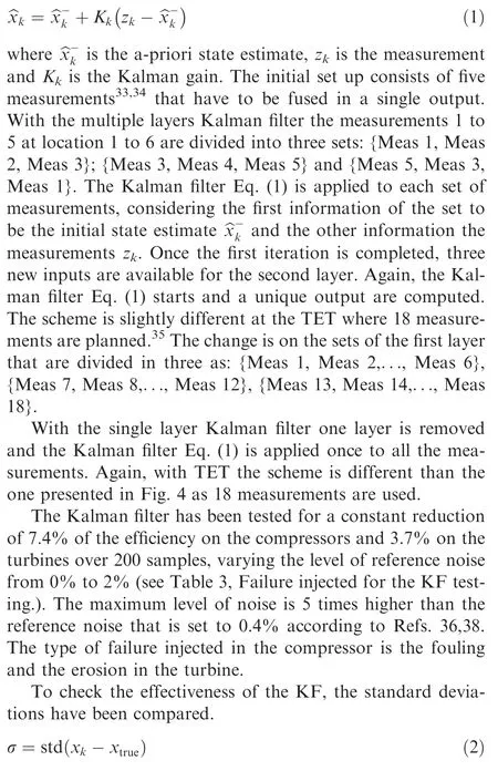
where xkis the real measurement after the KF,xtrueis the true reference without any noise and std is the equation used by MATLAB for the standard deviation calculation. According to Fig. A1 in the Appendix A, the MLKF with MM leads to a maximum reduction of 83% of the measurement standard deviation. The reduction moves to 76% if the SLKF with MM is used meaning that the second layer of the Kalman filter is worth 7% improvement. Instead, if the pressure is considered, the maximum reduction is 32% for MLKF with MM and 36% for SLKF with MM (it must be remarked that the noise level of the pressure is¼of the noise level of the temperature). This means that for the pressure the SLKF results in a higher reduction of the noise.However,the MLKF is better onoverall for all the measurements and at different noise levels(see Appendix A).

Table 3 Failure characterization.

2.3. Artificial neural network

The ANN is used to predict the efficiency of every single component and the deterioration parameters associated with it –mass flow, pressure ratio and efficiency decay. The type of ANN selected for this study is the cascade forward neural network that is working in a similar way as the feed-forward back propagation neural network but is adding a connection between the input and the n+1 layer. The neural network is set up in three layers that proved to be effective while keeping the computational time reasonable. The equation governing the artificial neural network is:

where W is the vector weight containing the input of each neuron and V is the vector. b is the bias assigned to each neuron and R are the number of entries. For a given problem, once the weight and the bias are established in the learning phase,the ANN is able to predict the output. The measurements included in the ANN are listed in Table 4 and are the result of the optimization performed during the testing phase. If‘‘No” is specified the measurement is not included, if ‘‘Yes”is specified the measurement is included

The pressure at the turbine exhaust p6is not included in the ANN because of the uncertainty even after the filtering shown in Fig. A2 in the Appendix A. The measurements of the first reference point and of the fuel mass flow are also ignored as they have been found less effective if included in the simulation.

For the given set of inputs in Table 4,the ANN is tuned to predict the efficiencies of the gas turbine components (LPC,HPC, HPT, LPT). The objective is to keep the deviations below a minor order of magnitude to rely on ANN as a model and do not affect the diagnostics because of model deviations.

Starting from the same failure characterization of Table 3,the maximum deviation on the predicted efficiency values,compared to the reference value of the model is 0.38% absolute at 2% measurement reference noise. The deviation isreduced to 0.14% absolute if the MLKF+ANN+FL is used (see Fig. A3).

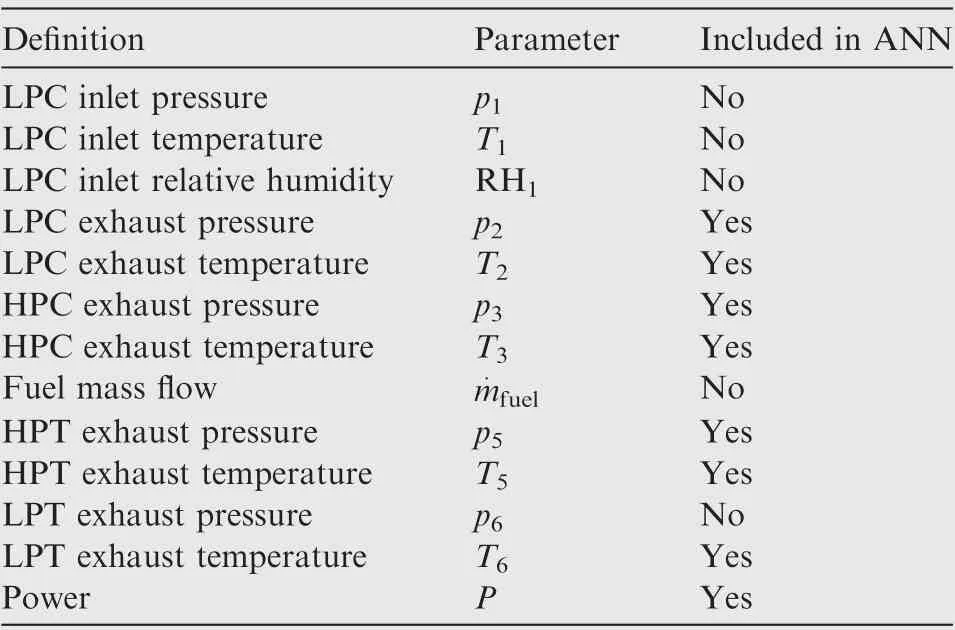
Table 4 Set of measurements included in the ANN.

2.4. Fuzzy logic

The fuzzy logic is used to quantify the severity of the failure of each component and to classify the type of malfunction. The quantification is based on the measurements data filtered in the KF module and on the efficiencies predicted in the ANN section. The FL must relate the cause-effect of each component to the severity of the failure.37To establish this relationship, eight cases, representative of single and multiple cases have been calculated (see Table 5).

The relationship out of the simulation done with the reference gas turbine presented in Performance modelling is shown in Table 6.From this matrix,it can be seen the effect the deterioration is playing on the affected components and the interaction with the other components. In case 4 for example –HPT erosion–the efficiency of the HPT decreases.The consequence is an increase of the HPC efficiency and a decrease of the LPC efficiency.

While establishing a direct cause-effect relationship and associating a severity level to it, the FL allows faster and unambiguous detection of the failures. The FL is set up in two sections: one for the quantification and another for the classification of the failures. The quantification relates the deterioration level to a magnitude that is set on a scale from 0 to 100. 0 represents the new engine without failures and 100 stands for the maximum level of deterioration recorded from the Refs. 23–32 and set up in the simulation. The relationship between the parameters in Table 6 and the FL magnitude is built with a neuro-fuzzy designer as shown in Fig. 5.The role of the ANN in this section is to tune, by modifying the weights,the fields of the FL.The classification is done with the FL and is tuned to classify the six types of failures listed in Table 5. The discriminant for the failure classification is the measurement,efficiency and deterioration reference level delta.This reference level delta, in particular, is the parameter used by the performance simulator (Turbomatch) to simulate a deteriorated engine. It includes mass flow, pressure ratio and efficiency impact, whose relationship varies depending on the type of failure considered. This information is calculated also from the ANN in its prediction phase.

The results of the quantification and classification are merged in a chart showing on the y axis the severity (quantification)and on the x axis the type of failure(classification).The severity is also associated with a colour code (traffic light) to facilitate the interpretation of the results (see Fig. 6).

3. Results

To test the robustness of the methodology dedicated tests have been conducted. The base for the test is the simulated engine described in Performance modelling. The main variables that are considered with the test are:

(1) Failure of one or multiple components.

(2) Variation of the degradation magnitude.

(3) Variation of the level of noise applied to the measurements.

To consider all these aspects,two sets of tests have been set:

(1) Constant deterioration with 7.4% degradation on the compressor and 3.7% on the turbine; multiple failures;variation of noise level (see Table 3).

(2) Random deterioration with degradation within 0.15%–7.4%; single, multiple and no failures; noise level 0.4%.

The output of the tests is the success rate.For the quantification,the simulated sample is counted if it lies within 3σ standard deviation,while the classification is counted if classified in the right category (also if outside the 3σ standard deviation).The standard deviation 1σ is calculated from a dry run with nominal noise (0.4%) and constant deterioration of multiple components. The calculated value is ±2.06 for 1σ, therefore,±6.18 for 3σ.

The results of the first test show a quantification above 99.5% for the nominal noise of 0.4% with all the combinations. With the maximum noise level of 2.0%, the success rate is decreased to 58.8%without the KF block.The rate increases to 72.4% if also the MLKF is employed and to 73.4% if the SLKF is used (see Table 7). However, it must be noticed that the MLKF+ANN+FL is performing better on overall reaching a maximum quantification success rate, with 2.0%noise, of 91.0% (see Fig. 7). The improvement after the data filtering is also visible in the decreased standard deviation seen in the quantification rate shown in Fig. A4.

The results of the classification with nominal noise (0.4%)show a success rate above 93.0% without filtering and at 100% with MLKF+ANN+FL (see Table 8). With the maximum noise, the success rate decreases to 86.0% if no fil-tering is used and increases again to 92.4% with MLKF+ANN+FL. Remarkable results are also achieved with SLKF+ANN+FL, where the minimum success rate is 90.9% with 2.0% measurement noise (see Fig. 8).

Table 5 Cases base of cause-effect scenario.

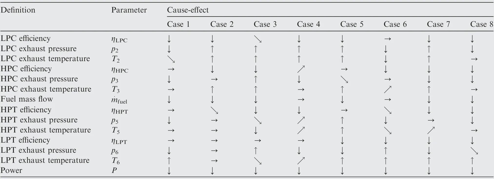
Table 6 Cause-effect for gas path parameters.

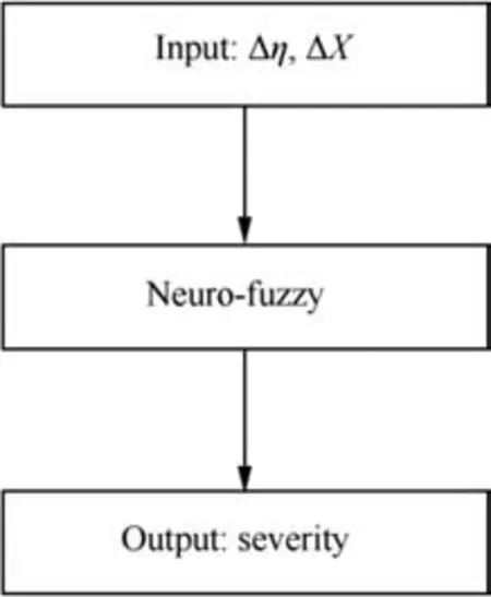
Fig. 5 Neuro-fuzzy designer structure.

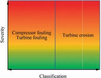
Fig. 6 Chart for quantification/classification of results.

The second simulation performed with random failures and degradation magnitude leads to a quantification rate above 92.0% (see Table 9). This result is obtained with the nominal reference noise of 0.4%.

The classification rate leads to a success rate above 95.1%(see Table 10).

The execution time per each sample point was also tested for the three combinations: (A) structure without Kalman filter; (B) structure with SLKF; (C) structure with MLKF. For the first case, the time per single point processed is 0.97 s, for the second the time is 1.1 s and for the third is 1.7 s. These results include the Kalman filter (if applied), the ANN prediction, the calculation of the reference value done with Turbomatch and the FL. The ANN training is excluded as it is done at an earlier stage with the previously calculated data.As the results are within seconds (1.7 s) this methodology results in being suitable for online diagnostics.

4. Discussion of results

The methodology structure has been clarified in the Problem formulation and consists of KF+ANN+FL. Each component of the methodology has been tested and the contribution has been measured.

In particular, the KF has been proposed in two ways:SLKF and MLKF. The SLKF leads to a maximum standard deviation reduction of 76% for the temperature and 36% for the pressure.The MLKF leads to a maximum standard deviation reduction of 83% for the temperature and 32% for the pressure. This difference is reflected in the overall quantification where the deterioration level is associated with severity based on a scale - fuzzy logic. The MLKF leads to a quantification success rate of 86.4%for LPC,82.4%for HPC,91.0%for HPT, 72.4% for LPT at 2.0% noise level (maximum rate considered). The SLKF leads to a quantification success rate of 82.4% for LPC, 75.4% for HPC, 83.9% for HPT, 73.4%for LPT at 2.0% noise level. The lower rate recorded is 73.4% and is a better result than the MLKF. However, the overall success rate is worse. For instance, the HPT is quantified with a rate of 7% higher with the MLKF. The case without filter leads to a quantification rate of 76.9% for LPC,58.8% for HPC, 66.3% for HPT, 63.3% for LPT which is the lower among the three configurations. This behaviour has been noticed early in the stages of this research and reflects the fact that for a valuable modelling via ANN and a positive quantification via FL, the data must be properly filtered.

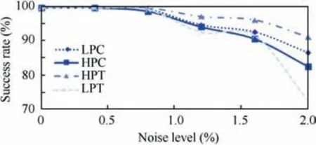
Fig. 7 Success rate for failure quantification (Combination MLKF+ANN+FL).

Focusing on MLKF(see Fig.7)a trend can be observed.In particular, the success rate decreases if the reference noise increases. This behaviour is expectable as the maximum noise level, 2.0% is 5 times higher than the nominal at 0.4%. For instance,2.0%noise corresponds to 15 K variation of the turbine exhaust temperature T6. The effect of the KF is a reduction of the slope of this trend obtained optimizing the KF parameters, so attenuating the noise.

Looking at the random simulation, the quantification success rate with 0.4%measurement noise is above 92.0%. However, this rate increases up to 99.0% on the LPT. With this simulation, every sample has a different type of failure and a different magnitude, therefore the high success rate confirms the robustness of the methodology.

The other parameter used to evaluate the robustness of the methodology is the classification rate. This parameter evaluates if the type of failure injected in the turbine is classified correctly meaning falling into the right category. As reported in fuzzy logic it relies on a standard fuzzy logic rather than the neuro-fuzzy logic used for the quantification. The minimum success rate values scored are 86.0% without any filter,90.9% with SLKF and 92.4% with MLKF. It is clear that the filter applied improves the classification rate and the MLKF results on being better than the SLKF. Looking at Fig.8 a decreasing trend related to the increase of the measurement noise can be observed. The bending is evident at 2.0%measurement noise, where the drop is 7% on the HPT and LPT. The HPC behaviour is an exception and is not strictly related to the MLKF. A similar attitude in-fact can be observed in the case without the KF and this is mostly driven by the ANN uncertainty prediction. The case with MLKF is better as it’s moving this transition toward the 2% measurement noise.

Table 8 Success rate for failure classification (unit: %).

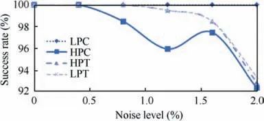
Fig. 8 Success rate for the failure classification (Combination MLKF+ANN+FL).

Table 9 Success rate for failure quantification for random simulation (combination MLKF+ANN+FL, Noise 0.4%).

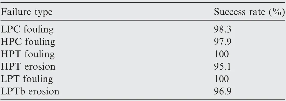
Table 10 Success rate for failure classification for random simulation (combination MLKF+ANN+FL, Noise 0.4%).

Looking at the second type of simulation, the minimum classification rate from the random case with nominal noise 0.4% is 95.1%. At every point of this simulation, the type of failure and the magnitude of the failure varies. It is clear that such a scenario is more critical than a real one and the success rate is lower than the single case failure. However, the high rate confirms the robustness of the methodology. This result is obtained with the MLKF in combination with MM. However, the Kalman filter coefficients have been tuned to give a response suitable for the type of problem. This was necessary as the Kalman filter is slow reacting if the measurement noise covariance is set to high values.In fact,being slow reactive it is advantageous to compensate for high noise with a problem that is regularly changing but is leading to a loss of information in this specific test where the type of failure is changing rapidly.

5. Conclusions

The scope of this paper has been studying and showing the results of a methodology for the performance-based diagnostics on a two-spool engine in the presence of measurement errors.

The research associated with the performance-based diagnostics is already extended as shown in Introduction.However,there are some clear areas of opportunity where this paper placed its target. The first is the multiple failure diagnostics in presence of measurement malfunctions.The second is the combination of multiple techniques that could make use of the mutual benefit providing a methodology that is robust over a wide range of conditions and flexible, so able to deal with different types of engines and with additional types of failure.

Looking at the significance of this methodology,the combination that has been proposed in this paper is KF+ANN+FL which is, as illustrated in Introduction, a methodology combining the strength of the three contributors.

To validate the methodology a model has been produced.This model is based on information available in the open literature.The information used is the key reference values like the efficiency of the components,power,mass flow and overall heat rate.In the same fashion,the deterioration profile is the result of the information available in the literature review and included in the performance model. On top of it, a reference noise has been added to each measurement. This set up has been prepared to make the simulation as realistic as possible.

Based on the objectives set at the beginning, the main results obtained are:

(1) The first contributor,the KF resulted in being beneficial reducing the standard deviation by a maximum of 83%.

(2) The ANN reached a very good match compared to the real value resulting in a maximum standard deviation of 0.38%.

(3) The data provided by the KF together with the prediction of the ANN set the base for reaching a success rate above 92.0% in terms of quantification and 95.1% in terms of classification in case of random simulation with variable deterioration magnitude and failure type.

(4) While challenged with a noise rate 5 times higher than the nominal noise 2.0% and constant degradation, the methodology still reached a quantification rate above 72.4% and a classification rate above 92.4%.

(5) The methodology resulting in being suitable for online diagnostics since the processing time per sample is 1.7 s.

With this work, scientific points in the performance-based diagnostics scenario have been investigated. Nevertheless, this specific methodology gives some additional opportunities for the research. Specifically, the measurement noise has been studied, but the measurement bias was not. This is a real scenario that can affect the results of the diagnostics. Moreover,the type of failures that have been investigated are two–fouling and erosion,leading to six-component failures–LPC fouling/HPC fouling/HPT fouling/HPT erosion/LPT fouling/LPT erosion. The FL, that has been placed for the classification,leave the opportunity to add new rules to detect other types of failure like clearance increase, flow bleeding and foreign object damage.

Acknowledgement

This paper is not supported by any sponsorship and relies on open literature information and on Cranfield in house tools for performance modelling.

Appendix A

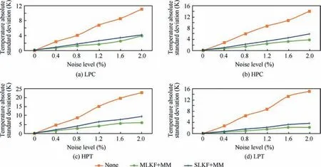
Fig. A1 Temperature absolute standard deviation for difference noise levels 0%–2%.

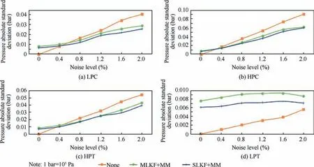
Fig. A2 Pressure absolute standard deviations for difference noise levels 0%–2%.

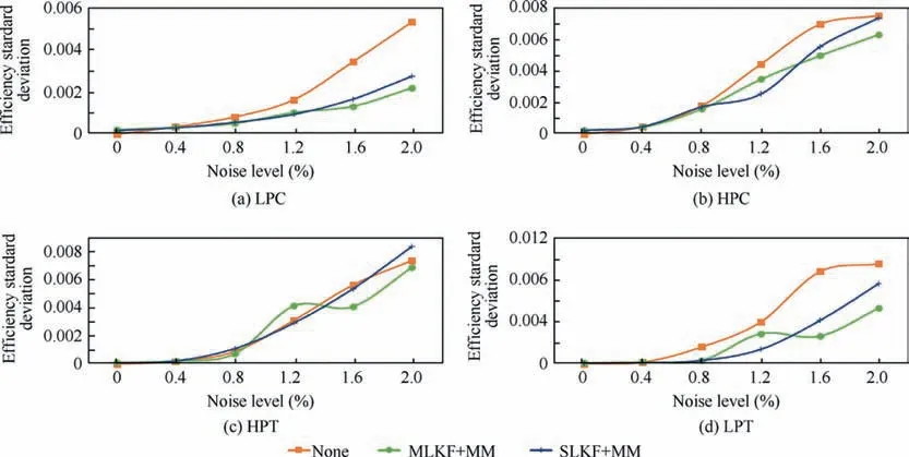
Fig. A3 Efficiency standard deviation for difference noise levels 0%–2%.

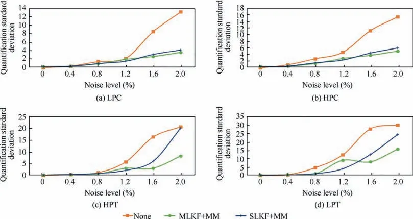
Fig. A4 Quantification standard deviation for difference noise levels 0%–2%.