Unstable unsteady aerodynamic modeling based on least squares support vector machines with general excitation

Senlin CHEN, Zhenghong GAO, Xinqi ZHU, Yiming DU, Chao PANG

School of Aeronautics, Northwestern Polytechnical University, Xi’an 710072, China

KEYWORDS Aerodynamics models;Forced vibration;Input design;Least squares support vector machines;Nonlinear system;System identification;Unsteady aerodynamics

Abstract Common, unsteady aerodynamic modeling methods usually use wind tunnel test data from forced vibration tests to predict stable hysteresis loop.However,these methods ignore the initial unstable process of entering the hysteresis loop that exists in the actual maneuvering process of the aircraft. Here, an excitation input suitable for nonlinear system identification is introduced to model unsteady aerodynamic forces with any motion in the amplitude and frequency ranges based on the Least Squares Support Vector Machines (LS-SVMs). In the selection of the input form,avoiding the use of reduced frequency as a parameter makes the model more universal.After model training is completed,the method is applied to predict the lift coefficient,drag coefficient and pitching moment coefficient of the RAE2822 airfoil, in sine and sweep motions under the conditions of plunging and pitching at Mach number 0.8.The predicted results of the initial unstable process and the final stable process are in close agreement with the Computational Fluid Dynamics(CFD)data,demonstrating the feasibility of the model for nonlinear unsteady aerodynamics modeling and the effectiveness of the input design approach.

1. Introductions

Aerodynamic modeling is the basis for aircraft simulation analysis and control system design. The traditional aerodynamic derivative model has been widely used in aircraft design.With the increased requirements for fighter performance, aircraft must be super-maneuverable. In this case, complex flow phenomena such as separated vortexes or shock waves,appear in the flow field, and the aerodynamic force exhibits obvious nonlinear and unsteady hysteresis characteristics; that is, the aerodynamic force will depend on the current state and time history of motion.1,2In such cases,it is difficult to apply traditional aerodynamic derivative models.3,4It is computationally expensive to use CFD methods for unsteady calculations,so it is necessary to explore accurate and efficient nonlinear,unsteady aerodynamic modeling methods.

Several studies5-7have been conducted on the mathematical modeling of nonlinear, unsteady aerodynamic forces. A brief overview of various methods is given here. Although the theoretical foundation of the step response model1,8is complete,the model structure is complex,and parameter identification is difficult. Volterra series model9,10is a nonparametric method based on input-output data. The logic of the model is clear and no specific flow mechanism needs to be considered. The disadvantage of the model lies in the large workload involving higher-order kernel identification and the sensitivity of the series model to the state change. State space model11,12describes flow field characteristics by introducing state variables that have clear physical meaning. However,the flow field structure is often complex and variable, which leads to a limited application scope for the model. State space model is mainly applied in aerodynamic modeling of the large angle of attack region of a triangular wing. Differential equation model13,14decomposes aerodynamic force into three parts: static, quasi-stationary increment and unsteady increment. Subsequently, the unsteady increment is approximately represented by first-order differential equations. The shortcoming of such a model lies in the need to identify aerodynamic derivatives and time constants at different angles of attack and reduced frequencies, resulting in a large number of identification parameters.Due to the lack of understanding and effective descriptions of the mechanisms behind the complex flow phenomena, these mathematical models have many problems associated with expressing nonlinear,unsteady aerodynamic forces.

With the rapid development of machine learning, there have been attempts to apply it to aerodynamic modeling in recent years, such as by applying neural network,15fuzzy logic,16and Support Vector Machine (SVM)17,18methods.The advantages of such methods are to treat the system as a black box without specific details that need to be considered. The SVM is based on the statistical learning theory for small sample cases that was proposed by Vapnik19in 1995. SVM was originally applied for pattern recognition and later extended to system identification, intelligent control,20,21and other fields. SVM uses structural risk minimization criteria to replace empirical risk minimization criteria,that are commonly used in neural networks and other methods. Thus, SVM seeks a balance between model complexity and learning ability based on limited sample information,effectively overcoming over learning issues of neural networks and dependence on the experience of fuzzy logic. Least Squares Support Vector Machines (LS-SVMs)22are an improved version of the standard SVM, which transform the quadratic programming problem into linear equations solutions, thus reducing the computational complexity. In this paper, it has been selected for unsteady aerodynamic modeling.

Most of the existing unsteady aerodynamic modeling methods use wind tunnel test data from forced vibration tests. The schematic diagram is shown in Fig.1.At a certain reduced frequency, after the test object moves for a period of time, the flow tends to be stable, following which the stable hysteresis loop data is collected as the sample output. Subsequently,the experiment is carried out at another reduced frequency.After the test is completed, the stable hysteresis loop data is obtained at several reduced frequencies. Following this, the modeling is carried out according to this training data. After the modeling is completed, the model is used to predict the aerodynamic response at other reduced frequencies.

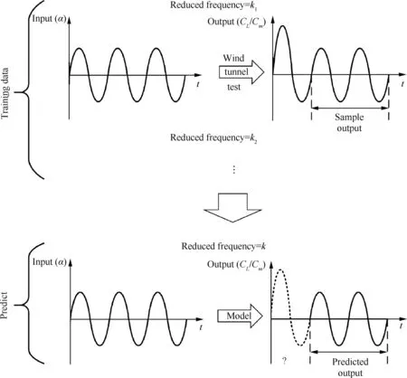
Fig. 1 Schematic diagram of common aerodynamic modeling method based on wind tunnel test data.

Based on this idea, some methods17have been applied successfully. However, the modeling objects of these methods are always stable hysteresis loops.However,these methods do not take the initial stage of aerodynamic force into account, i.e.,the process of entering the stable hysteresis loop.Nevertheless,it is almost impossible for the actual maneuver of the aircraft to have a stable vibration with constant frequency, for example,continuous sine or cosine motion,but instead is a dynamic changing process. In other words, focus is to be placed on unsteady aerodynamic performance, when the aircraft is maneuvered rapidly. It can be assumed that the aircraft will not continue to move to a stable hysteresis loop, but is always in the initial stage. Therefore, the aerodynamic force prediction of the initial stage is more valuable than that of the stable stage.Taking the RAE-2822 airfoil for example,the lift coefficient hysteresis loop of the airfoil calculated by CFD with different reduced frequencies in pitching motion at transonic velocity is shown in Fig. 2. In the graph, the solid lines are the stable hysteresis loop,and the dotted lines represent the initial stage of the airfoil entering the hysteresis loop. It is found that an aerodynamic force obviously exists during the process of entering the stable hysteresis loop. Therefore, it is not enough to predict the stable hysteresis loop,and it is necessary to construct an aerodynamic force model which can reflect the initial unstable process.

Here, an orthogonal phase-optimized multisine input suitable for nonlinear system identification is designed to replace the common forced vibration input. By using CFD, all data containing the initial motion are collected, so aerodynamic modeling with the initial changing process is realized. In this case, only one excitation is needed to predict any input in the amplitude and frequency ranges. This method does not require multiple forced vibration data, reduces computational complexity, and can predict motions other than vibration.Additionally, the selection of input form is important and directly influences the prediction accuracy. Because the actual flight process cannot be represented using standard oscillating motion, this paper abandons the common parameter of reduced frequency. According to the dependence of the aerodynamic force on the motion process, the input form is selected,and a general aerodynamic model that is independent of the frequency and can reflect the process of arbitrary motion is established.

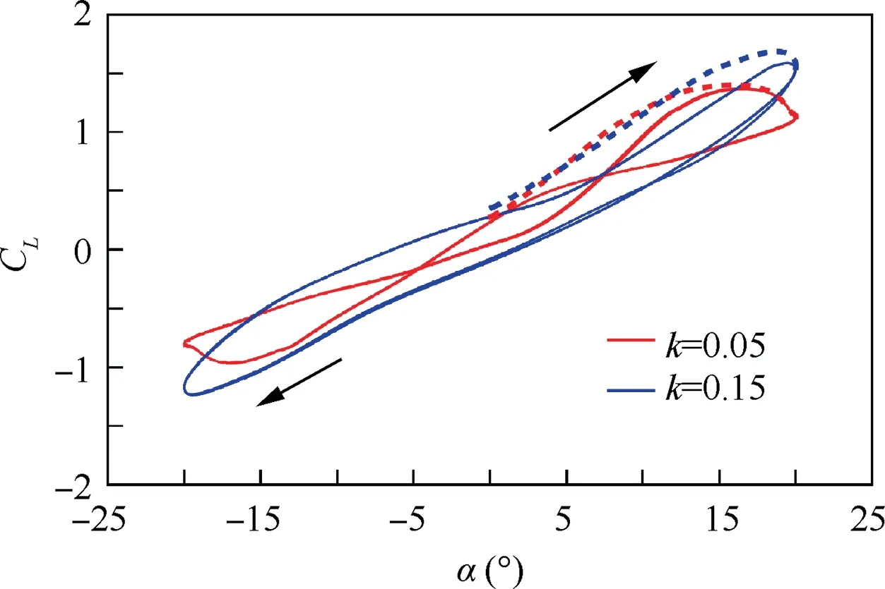
Fig. 2 CFD data of lift coefficient of RAE2822 airfoil for pitching motion with reduced frequency of k=0.05 and k=0.15,at Ma∞=0.8 and Re=6.3×106.

In this paper, an excitation input is designed for nonlinear unsteady aerodynamic modeling including the initial unstable process based on the LS-SVM. Initially, the shortcomings of forced vibration based on the wind tunnel test, selection and design of inputs for excitation, and selection of input forms for training are discussed. Subsequently, the basic theory and parameter determination method of the LS-SVM are introduced. Following this, the aerodynamic data obtained by CFD are used for training. Finally, the prediction ability of the method in this paper is verified based on the aerodynamic force of the airfoil in sine motion and sweep motion under plunging and pitching conditions.

2. Input

2.1. Discussion about forced vibration input

The commonly used aerodynamic modeling input was the‘‘stable”aerodynamic wind tunnel test data from forced vibration tests.When the object was moving,the aerodynamics was unsteady.When the object moved regularly,the aerodynamics would gradually tend to change regularly. The unsteady aerodynamics with regular changes could be called‘‘stable”.There were some shortcomings in this method of predicting hysteresis loop using a hysteresis loop.

Initially,the response of the system to forced input was discussed.Taking a typical linear oscillator system as an example,the equation of motion was shown as

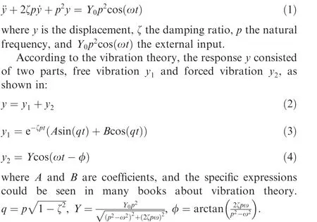
For a stable system,the free vibration y1gradually decayed to zero over time,leaving only the forced vibration y2.Taking an oscillator23for example, the responses for free and forced vibrations under sinusoidal excitation are shown in Fig. 3.The traditional unsteady aerodynamic modeling17based on wind tunnel test only used stable, unsteady aerodynamic data,but neglected the initial changing process, i.e., only data from forced vibration was used, and data from free vibration was ignored. This would result in the loss of information about the evolution of the system response. Therefore, the model based on this data could only predict the final stable hysteresis loop, and could not predict the initial unstable process of entering the hysteresis loop.

Following this,the actual process of maneuvering flight was discussed.It was almost impossible for the actual flight process to have standard oscillatory motion, and naturally there was no single frequency. However, most of the existing methods took the reduced frequency as a model parameter. So these methods could be difficult to use to predict the aerodynamic forces involved in the real flight process,i.e.,arbitrary motion.In view of these,the design of the input signal and selection of input form were studied in this paper.

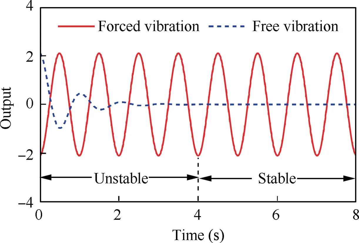
Fig. 3 Forced and free vibration response of an oscillator23 under sinusoidal excitation.

2.2. Selection and design of excitation input

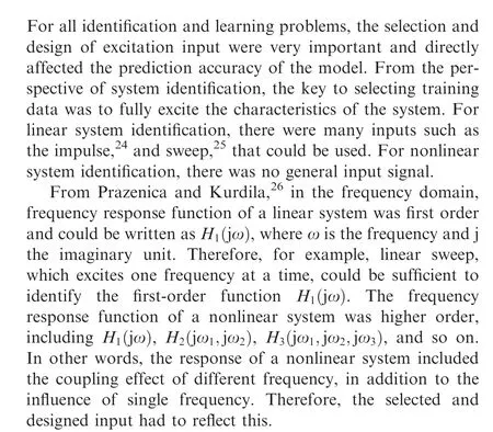
In this paper, an orthogonal phase-optimized multisine input designed by Morelli et al.27,28for the coupled excitation of multi-effector of an aircraft was used as the training input.The input was a superposition of selected orthogonal harmonic sinusoids and could reflect the coupling of different frequency.It is suitable for the identification of nonlinear systems. Chen and Gao29successfully applied this input to the identification of Volterra higher-order kernels for nonlinear aerodynamic modeling of airfoils in the range of small angles of attack at transonic velocity.

The expression of the orthogonal phase-optimized multisine input was

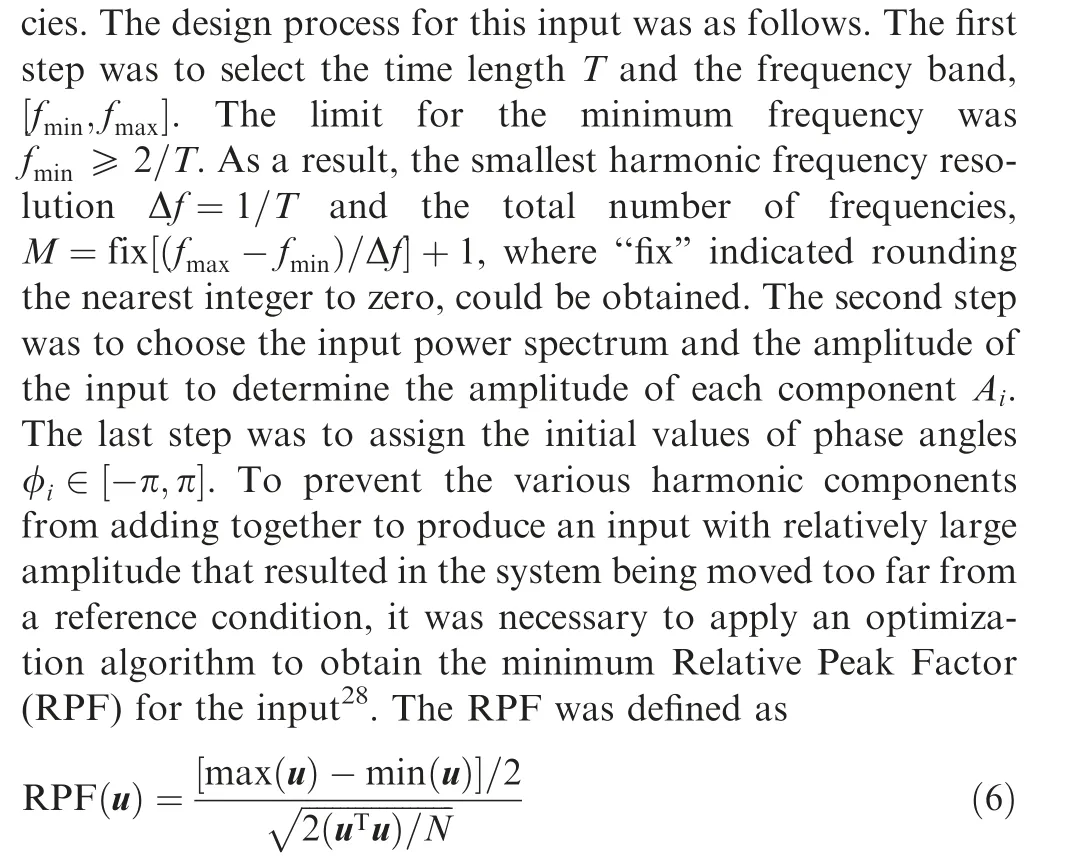
where N is the number of discrete input points.

The first two seconds of the orthogonal phase-optimized multisine input used for identification in this paper is shown in Fig. 4, where T=20 s, fmin=3/20 Hz, and fmax=30 Hz.

2.3. Selection of input form for training

Before training, it was necessary to choose a reasonable input form according to the physical background of the actual problem.Because the unsteady aerodynamic force depended on the previous motion process in addition to the current motion state,the selection of the input form must reflect this.In many studies involving machine learning in aerodynamic modeling,the reduced frequency or artificially defined equivalent reduced frequency was often regarded as one of the input parameters.Notably,most of the training data came from forced vibration wind tunnel tests at different reduced frequencies, as noted by Ignatyev et al.30and Wang et al.17.In the actual flight process of an aircraft, it was almost impossible to achieve standard oscillatory motion,so there was no fixed frequency.Establishment of an aerodynamic model that was independent of frequency and had universal significance was one of the problems studied in this paper.

The input form for training used in this paper was as follows:

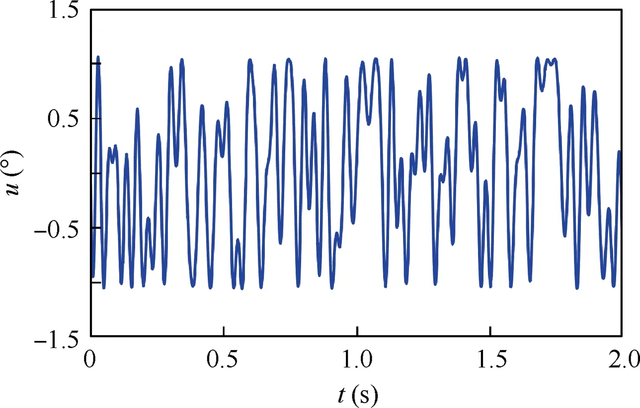
Fig. 4 Orthogonal phase-optimized multisine input (first two seconds).

where α is the angle of attack and m the time-dependent length of the aerodynamic force at the current moment in relation to the previous motion process. The reduced frequency was not introduced here because the influence of the frequency was considered in the design of the excitation signal, via the selection of the frequency band.

3. Least squares support vector machines

3.1. Basic theory

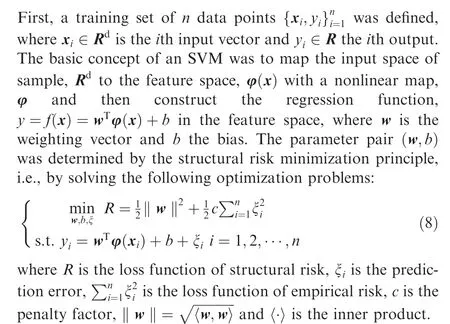
The traditional learning method was mainly based on the principle of empirical risk minimization, which obtained the least empirical risk for a given sample set.In theory,the empirical risk converged to the real risk when the sample data used for training tended to infinity.However,in practical problems,the number of samples was generally limited, and the minimum empirical risk did not always reflect the minimum real risk. Therefore, many algorithms based on this principle, such as neural networks,often had the problem of‘‘over learning”.According to the statistical learning theory, the real risk of learning machines included empirical risk and a confidence range.To reduce the real risk,the confidence range and empirical risk would have to be reduced to a feasible extent. The confidence range was related to the complexity of the learning machine and the number of training samples. Under the condition that the number of samples remained the same,a reduction in the confidence range would reduce the complexity.Reducing ‖w‖ could reduce the complexity, so ‖w‖2/2 was treated as part of Formula (8).

The Lagrangian function method was introduced to solve the equality-constrained optimization problem in Eq. (8):

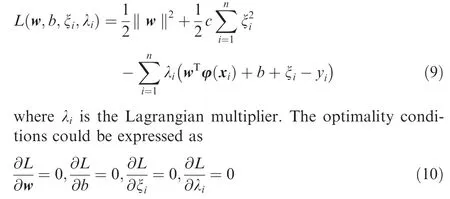
By solving Formula (10), the following equations could be obtained:

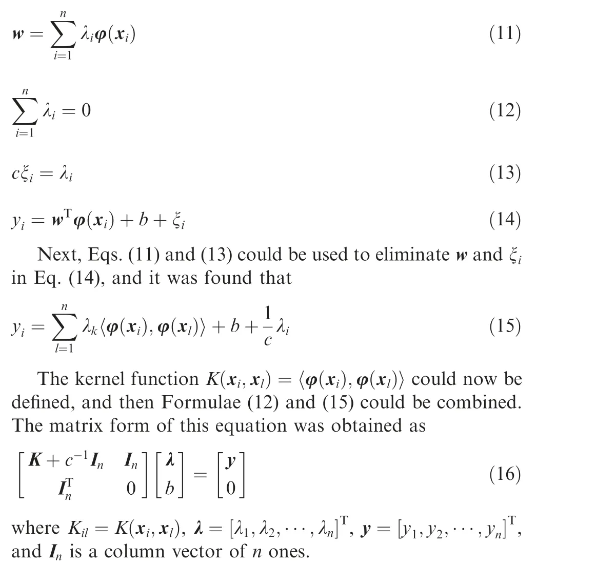
The optimal parameters （λ ，b）could be obtained by solving Formula (16) directly. A more efficient method was to use the symmetric positive-definite property of the kernel function matrix K to transform the system of equations and subsequently use Cholesky decomposition to solve it. The specific method was proposed by Cawley and Talbot31. After the set（λ ，b） was obtained, the required LS-SVM model could be obtained as

3.2. Determination of model parameters

By introducing the kernel function,an SVM avoided the direct calculation of the inner product in a high-dimensional feature space, which greatly simplified the calculations. According to functional theory, any symmetric function that satisfied the Mercer condition could be regarded as a kernel function,and the Gaussian kernel function was most commonly used.

After the kernel function was selected,the determination of model parameters mainly included the determination of the kernel parameter σ and the regularization parameter c. The generalization error corresponding to a group of parameters（σ ，c） was usually calculated by the leave-one-out crossvalidation method. Given a set of parameters （σ ，c）, each time one of the training samples was used as a test set,the rest were used as a training set, and the prediction error was calculated.This process was repeated until each sample was used as a test set. Finally, the average value of all prediction errors was taken as the generalization error for this set of parameters.The ‘‘fmincon” function in the optimization toolbox of MATLAB could be used to find the parameters that minimized generalization error.31

3.3. Training method

After the excitation input was selected,the aerodynamic forces were calculated with CFD. Subsequently, the input vector xiwas constructed according to the selected input form, and the outputs included the lift coefficient, drag coefficient, and pitching moment coefficient. Finally, the LS-SVM model was trained and the specific steps were as follows.

Step 1 According to the input constructed in Section 2.2,the aerodynamic forces were calculated by CFD.

Step 2 The input vector xiwas constructed according to Section 2.3 and the output yiwas the aerodynamic force,where i=1，2，···，n.

Step 3 The initial values for the model parameters,c in Formula (8) and σ in Formula (18), were given.

Step 4 The average prediction error calculated by the leaveone-out cross-validation method was used as the optimization target to find the optimal model parameters （σ ，c）, with the‘‘fmincon” function in MATLAB.

Step 5: Steps 3 and 4 were revisited a number of times to avoid local optimization, and the model parameters that minimized the average prediction error were selected.

Step 6: Formula (16) to obtain the parameters （λ ，b） was solved and training of the model was finished. After the test input was provided, the prediction result of the model could be calculated with Formula (17).

4. Training with RAE2822 airfoil

This paper considered the plunging and pitching motion of an RAE2822 airfoil at transonic velocity as examples, to verify the ability of the LS-SVM to predict nonlinear unsteady aerodynamic force and validate the effectiveness of the designed input. CFD provided the training data and was independent of any specific method. The flow conditions were Mach number Ma∞=0.8 and Reynolds number Re=7.2×106, and a rigid dynamic grid was used. The sample grid generated around the airfoil is shown in Fig. 5.

4.1. Validation of flow solver

To verify the CFD flow solver,Cases 3,9 and 10 with different flow conditions for the RAE-2822 airfoil were studied, as established by Cook et al.32.The first case was Case 3,in which the flow conditions were Mach number Ma∞=0.6, Reynolds number Re=6.3×106, and angle of attack α=2.57◦. The second case was Case 9, in which the flow conditions were Mach number Ma∞=0.73, Reynolds number Re=6.5×106, and angle of attack α=3.19◦. The third case was Case 10, in which the flow conditions were Mach number Ma∞=0.75, Reynolds number Re=6.2×106, and angle of attack α=3.19◦. The pressure coefficient Cpdistribution of the CFD results, based on the constant lift coefficient method and the wind tunnel test results, were compared as shown in Fig. 6. It could be found that the CFD results were in good agreement with the wind tunnel test results. Even if shock waves appeared in Cases 9 and 10, the positions of the shock waves calculated by CFD were consistent with those from the wind tunnel tests.A comparison of the lift coefficient,drag coefficient, and pitching moment coefficient is shown in Table 1. When the lift coefficient was fixed, the CFD results for the drag coefficient and pitching moment coefficient in the three cases were generally consistent with the wind tunnel test results.Some deviations could be observed in the comparison of test results and were within the allowable error range.The reliability of the CFD solver was verified through the comparison of the pressure coefficient distribution and aerodynamic coefficients in the three cases. The static aerodynamic forces of the RAE2822 airfoil at a Mach number of Ma∞=0.8 and Reynolds number of Re=6.3×106are shown in Fig. 7.

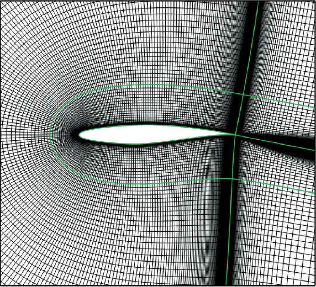
Fig. 5 Sample grid generated around RAE2822 airfoil.

4.2. Validation of training data

After the training was completed, the training data were used as test samples to test the training effect. Fig. 8 illustrates the LS-SVM prediction results and CFD calculation results for the lift coefficient, drag coefficient, and pitching moment coefficient of the airfoil, in plunging and pitching motions, respectively. The maximum equivalent angle of attack of plunging motion was 20°,and the maximum angle of attack of pitching motion was 20°. For the selection of time-dependent length in Formula (7), it was necessary to try different lengths, m, of time and then choose the optimal value according to the training error. Here, the plunging motion used m=25, and the pitching motion used m=15.Fig.8 shows that the prediction results were in good agreement with the CFD results, and the learning ability of the LS-SVM based on the training data was verified.

5. Results and discussion

After the model training was completed, it was necessary to verify the prediction accuracy for other inputs, i.e., to verify the generalization ability of the model.In this paper,the aerodynamic forces of the airfoil for sine motion and sweep motion under plunging and pitching conditions were calculated and verified.

5.1. Plunging motion

Fig. 6 Pressure coefficients distribution of RAE2822 airfoil.

Table 1 Comparison of CFD results and wind tunnel test results.

Fig. 7 Aerodynamic coefficients of RAE2822 airfoil at Ma∞=0.8 and Re=6.3×106.

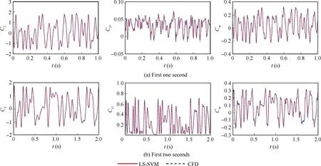
Fig. 8 LS-SVM predictions and training data in pitching motion.

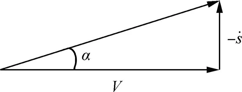
Fig. 9 Schematic diagram of equivalent angle of attack.

Only the angle of attack changed when the airfoil moved up and down in plunging motion, as shown in Fig. 9. Taking the angle of attack as an independent variable,the relationship between the angle of attack and displacement was as follows:

where V is the free stream velocity,α the angle of attack,and s the displacement of the airfoil. The variation of the angle of attack was based on an orthogonal phase-optimized multisine function with an amplitude of 20°.

The test motions that corresponded to the variations in the angle of attack of the airfoil when the initial angle of attack was 0° were as follows:

The corresponding displacement variation was calculated using Formula (19). In Formula (20), the first two equations were associated with sinusoidal motion,and the corresponding reduced frequencies were 0.05 and 0.15,respectively.The third equation represented sweep motion, and the corresponding reduced frequency increased linearly from 0 to 0.08.

The results of the test motions predicted with the LS-SVM were compared with the CFD results,as shown in Fig.10.The aerodynamic prediction results under both the sinusoidal motions were in good agreement with CFD results. It could be found that the aerodynamic force was stable after a period of time, following which the cycle was repeated. The differences between the initial and stable stages of the lift and drag coefficients were small, and the difference between the initial and stable stages of the pitching moment coefficient was obvious.Thus,accurate prediction of the aerodynamic force in the initial unstable stage was realized in addition to accurate prediction of the aerodynamic force in stable stage.

In terms of nonlinearity, the degree of nonlinearity of the lift coefficient was the weakest and prediction precision was the highest, among the two types of sinusoidal motion.Although the pitching moment coefficient displayed a visible nonlinear feature, the prediction results accurately showed local fluctuations in the corresponding position.The nonlinear characteristic of the drag coefficient was the most obvious;however, the prediction results still reflected corresponding motion trends. In the two types of sinusoidal motion, the degree of nonlinearity of the aerodynamic coefficient with a reduced frequency of 0.05 was higher than that of the aerodynamic coefficient at a reduced frequency of 0.15, i.e., the nonlinearity of the aerodynamic coefficient at a lower frequency was stronger than that at a higher frequency,so the prediction accuracy of the model at a lower frequency was relatively low.

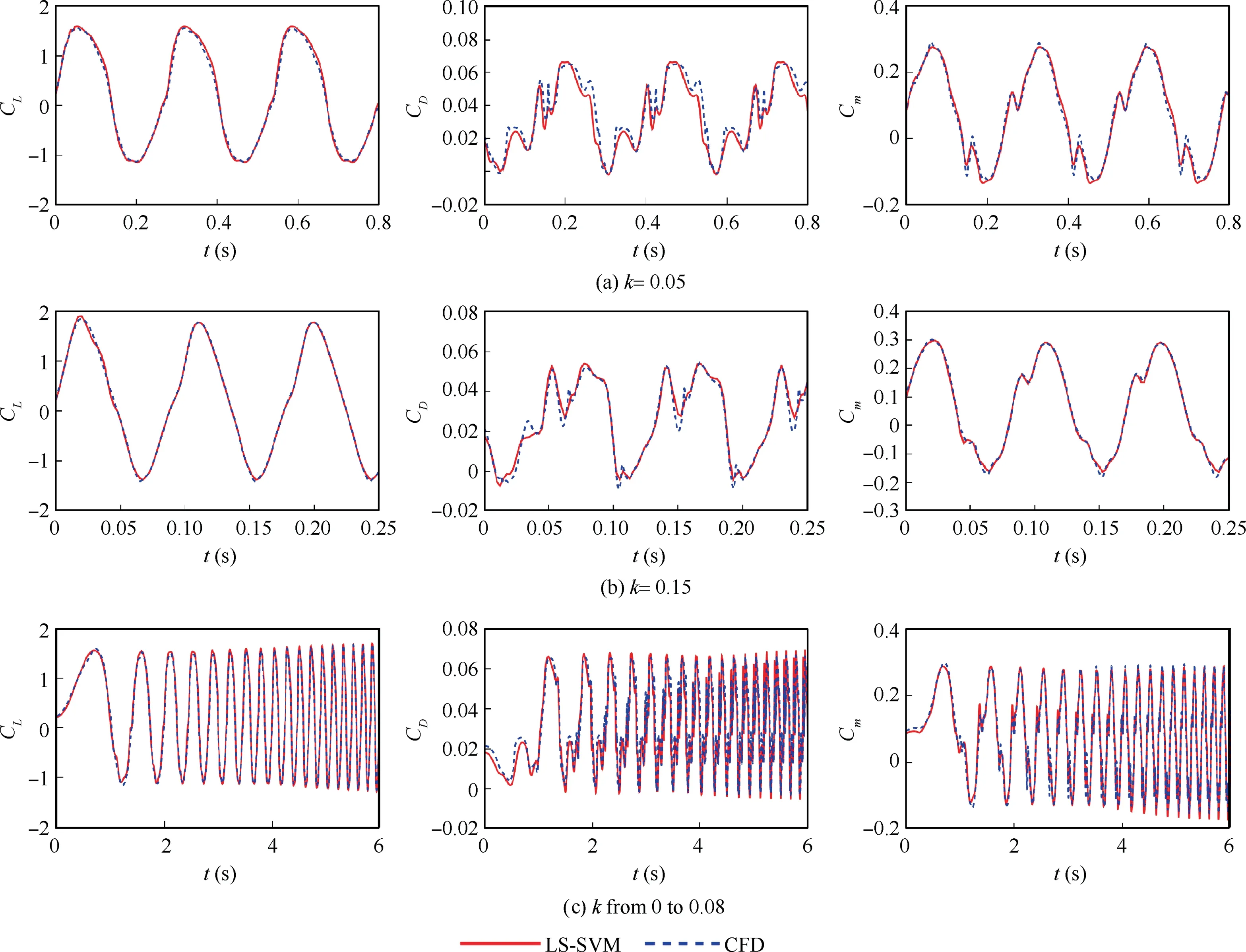
Fig. 10 LS-SVM predictions and CFD data in plunging motion.

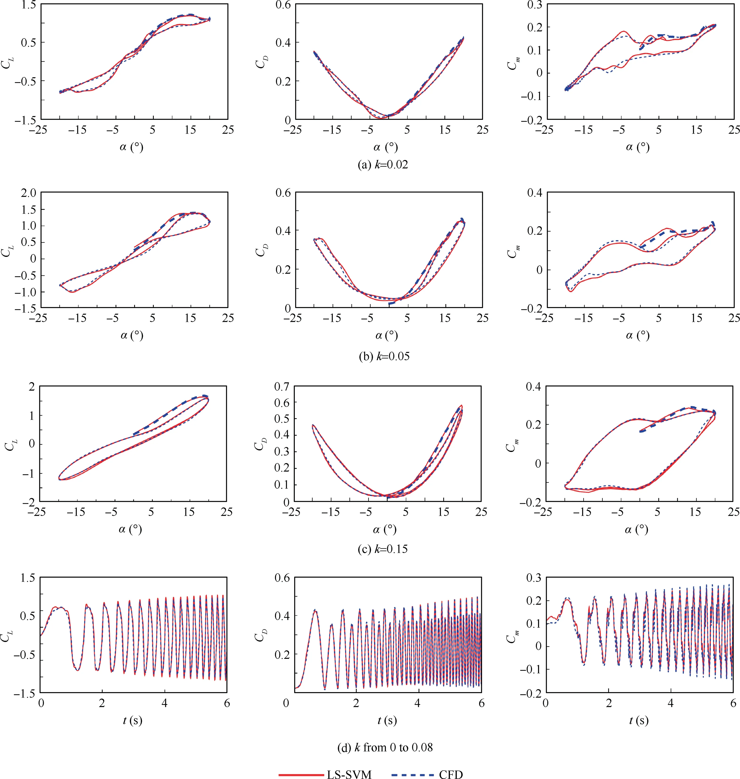
Fig. 11 LS-SVM predictions and CFD data in pitching motion.

In addition to the results discussed above, the prediction results for sweep motion were in good agreement with the CFD results. By using the proposed method for training and input form selection, reduced frequency was avoided as a parameter.Thus,both sinusoidal motion and arbitrary motion in the range could be theoretically predicted, which made the model more universal.

5.2. Pitching motion

The accuracy of the nonlinear, unsteady aerodynamic model predictions was verified under pitching conditions. The training inputs were orthogonal phase-optimized multisine data,and the amplitude of the angle of attack was 20°. The variations in the angle of attack of the airfoil when the initial angle of attack was 0° were as follows:

The reduced frequencies of the first three sine motions were 0.02, 0.05 and 0.15, and the reduced frequency of the fourth sweep motion varied from 0 to 0.08.

The results of the test motions predicted with the LS-SVM were compared with the CFD results,as shown in Fig.11.The prediction results of the hysteresis loop of the aerodynamic force in three types of sinusoidal motion were in good agreement with CFD results. The dotted and thickened lines represent the initial stage of entering the stable hysteresis loop.When the reduced frequency was 0.02, the initial stage of the aerodynamic force was not obvious, but at the reduced frequency of 0.05 and 0.15, the initial stage of the aerodynamic force was obvious.It could be seen that the process of entering the hysteresis loop had been accurately predicted in addition to prediction of the stable hysteresis loop.

Besides, the results for sweep motion were also in good agreement with the CFD results.In this case,the same conclusions that were obtained for plunging motion were applicable.Using the proposed method for training and input form selection, reduced frequency was avoided as a parameter. Thus,both sinusoidal motion and arbitrary motion in the range could be theoretically predicted.

5.3. Pitching motion with forced vibration as input

The following is a validation of the effect of aerodynamic prediction with forced vibration as input,discussed in Section 2.1.The third motion in Formula (21) was selected. The curve of variation of three periods of lift coefficient calculated by CFD is shown in Fig.12.The aerodynamics tended to change quickly at periodic intervals, and it could be assumed that the aerodynamics of the latter two periods were stable. The stable vibration data of the latter two periods, and overall vibration data across three periods, including the initial changing process,were used for training,respectively.Subsequently,the lift coefficient under the same input was predicted. The hysteresis loop curve of the prediction results is shown in Fig. 13. The curve corresponding to‘‘stable input”was the prediction result after training with the vibration data of the latter two periods.The curve corresponding to‘‘overall input”was the prediction result after training with the vibration data of three periods.

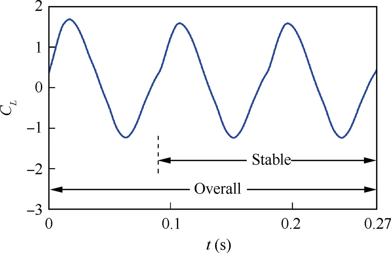
Fig.12 Training data of lift coefficient for pitching motion from CFD with a reduced frequency of k=0.15.

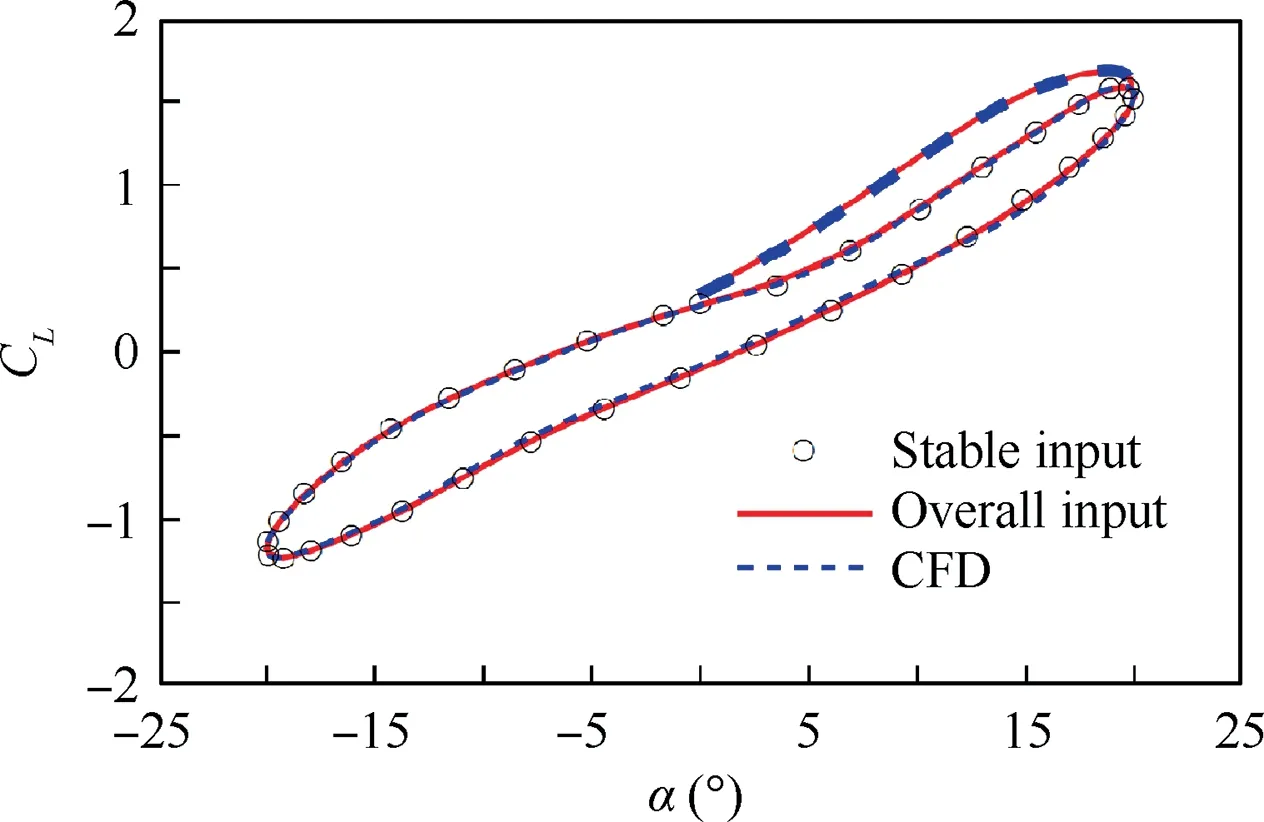
Fig.13 LS-SVM predictions and CFD data of lift coefficient for pitching motion with a reduced frequency of k=0.15 and different training input.

By comparing with the CFD data, it could be found that the stable hysteresis loop could be predicted using stable vibration for training,and the initial process of entering the hysteresis loop could not be predicted. The whole aerodynamic development process could be predicted by training with data containing the initial changing process. This example showed that the stable forced vibration data could only predict the stable hysteresis loop,and only if the initial free vibration data was included, the process of entering the hysteresis loop could be predicted.It was almost impossible for aircraft motion to be at standard vibration, but it was in the process of continuous change. Therefore, the modeling method of forced vibration,based on the wind tunnel test, would be difficult to predict aerodynamic force during aircraft maneuvering.

6. Conclusions

(1) In this paper, the LS-SVM was used for nonlinear,unsteady aerodynamic modeling. The accurate predictions of the lift coefficient,drag coefficient,and pitching moment coefficient under sine and sweep motions of RAE2822 airfoil in the transonic region indicated the ability of the method to effectively model nonlinear,unsteady aerodynamic forces.

(2) The verification results showed that the traditional modeling method based on wind tunnel test data from forced vibration tests, could only predict the stable hysteresis loop, but could not predict the initial unstable process of entering hysteresis loop, which was important in the actual maneuvering of the aircraft.

(3) By designing a training input suitable for nonlinear system identification and selecting reasonable input form,the hysteresis loop which contained the initial process could be predicted,together with avoiding consideration of frequency as the model parameter, thereby enabling arbitrary motion in the amplitude and frequency range to be predicted.