Exact surface energy and elementary excitations of the XXX spin-1/2 chain with arbitrary non-diagonal boundary fields

Jia-Sheng Dong(董家生), Pengcheng Lu(路鹏程),2, Pei Sun(孙佩), Yi Qiao(乔艺),Junpeng Cao(曹俊鹏), Kun Hao(郝昆),4,5, and Wen-Li Yang(杨文力),4,5

1Institute of Modern Physics,Northwest University,Xi’an 710127,China

2Beijing National Laboratory for Condensed Matter Physics,Institute of Physics,Chinese Academy of Sciences,Beijing 100190,China

3School of Physics,Northwest University,Xi’an 710127,China

4Peng Huanwu Center for Fundamental Theory,Xi’an 710127,China

5Shaanxi Key Laboratory for Theoretical Physics Frontiers,Xi’an 710127,China

6School of Physical Sciences,University of Chinese Academy of Sciences,Beijing 100049,China

7Songshan Lake Materials Laboratory,Dongguan 523808,China

Keywords: quantum spin chain,integrable systems,Bethe ansatz

1. Introduction

Exact solvable models are an important class of models in physics,which not only explain the mechanisms of many important physical phenomena,[1,2]but also are closely related to many fields in physics, such as quantum optics,[3]statistical physics[4]and the AdS/CFT correspondence.[5]The quantummechanical model of magnetism proposed by Heisenberg[6]was certainly the most important integrable system. Eigenvectors and the corresponding eigenvalues of the completely isotropic spin-1/2 Heisenberg model in one-dimension with periodic boundary condition were found in the pioneering work[7]by Bethe in 1931. After that, there have been many important advances in the study of the model,[8–11]one of which is impressive that the spin chain with arbitrary boundary fields was proven to be integrable.[12]Due to the existence of non-parallel boundary fields,the U(1)symmetry of the model is broken,so the conventional Bethe ansatz methods cannot be used to solve it.[13–15]In 2013,by using the off-diagonal Bethe ansatz method(ODBA),[16,17]the spectrum of this model was given by an inhomogeneousT–Qrelation.[18,19]However,due to the existence of inhomogeneous terms in the Bethe ansatz equations(BAEs),the physical properties of the model cannot be obtained directly by using the thermodynamic Bethe ansatz method(TBA).[20,21]

In response to this problem,a series of important progress has been made recently.Firstly,Jianget al.[22]showed that for the isotropic spin-1/2 chain with arbitrary boundary fields,the two boundaries are decoupled from each other completely in the thermodynamic limit. In addition, Nepomechieet al.[23]derived an expression for the leading correction to the boundary energy in terms of the boundary parameters. Wenet al.[24]showed that the inhomogeneous term in theT–Qrelation can be ignored in the thermodynamic limit and derived the boundary energy by using the TBA method within a certain boundary parameter region. For theXXZspin chain with arbitrary non-diagonal boundary fields,Qiaoet al.[25]gave the surface energy and elementary excitations by using the zero roots of the transfer matrix. For the antiperiodicXXZspin chain, Leet al.[26]proposed an analytic method to derive the patterns of the zero roots of the transfer matrix in the thermodynamic limit. These methods made it possible to study the surface energy and elementary excitations of the quantum integrable systems without U(1)symmetry.

In this paper, we shall investigate some physical properties of theXXXspin-1/2 chain with arbitrary non-diagonal boundary fields. We find that with the analysis of the BAEs (32), we can get the general zero root patterns of the transfer matrix. Then, according to the numerical analysis of the exact diagonalization of the model, we give the specific distribution of the zero roots corresponding to the ground state of the model under different boundary field conditions in Table 1.Based on these,as well as a set of auxiliary inhomogeneity parameters and the relations(23)satisfied by the eigenvalue of the transfer matrix, we obtain the surface energy and elementary excitations of the model. This paper is organized as follows. We briefly give some reviews about the integrability of the isotropic spin-1/2 chain with arbitrary non-diagonal boundary fields in Section 2. In Section 3, we consider the case of diagonal boundary fields and analyze the root patterns of the eigenvalue of the transfer matrix. Then, we calculate the corresponding ground state energy. In Section 4 we consider the case of arbitrary boundary fields and solve the surface energy and elementary excitations of the model. Finally,we summarize our work in Section 5.

2. Integrability

Throughout,Vdenotes a two-dimensional linear space and let{|m〉,m=0,1}be an orthogonal basis of it. We shall adopt the standard notations:for any matrixA ∈End(V),Ajis an embedding operator in the tensor spaceV ⊗V ⊗···,which acts asAon thej-th space and as identity on the other factor spaces. ForB ∈End(V ⊗V),Bi jis an embedding operator ofBin the tensor space, which acts as identity on the factor spaces except for thei-th andj-th ones.

Let us introduce theR-matrixR0,j(u)∈End(V0⊗Vj)

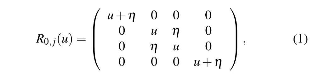
whereuis the spectral parameter. TheR-matrix (1) satisfies the following relations:

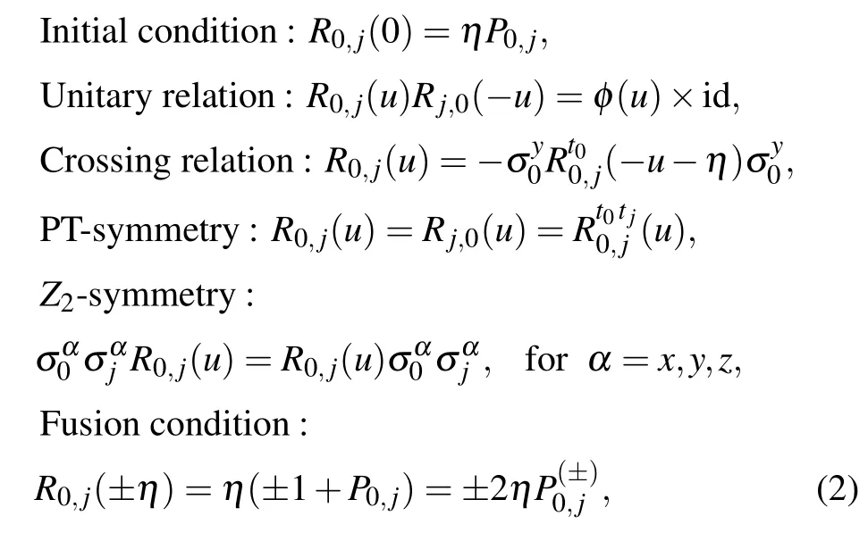
whereφ(u)=η2-u2,t0(ortj) denotes the transposition in the spaceV0(orVj)andP0,jis the permutation operator possessing the property

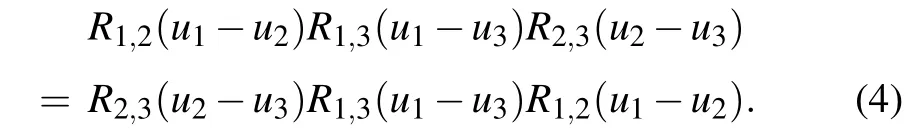
TheR-matrix(1)satisfies the quantum Yang–Baxter equation(QYBE)

We define the monodromy matrices as

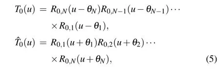
whereV0is the auxiliary space,V1⊗V2⊗···⊗VNis the physical or quantum space,Nis the number of sites and{θj|j=1,···,N}are the inhomogeneity parameters.

The reflection matricesK±(u)read

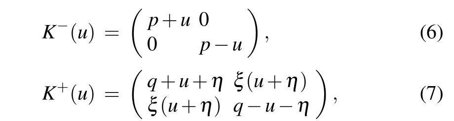
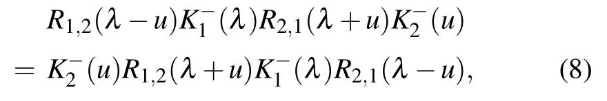
whereηis the crossing parameter,andp,q,ξare the boundary parameters associated with the boundary fields. TheKmatricesK±(u)satisfy the reflection equation(RE)

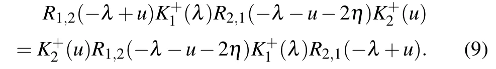
and the dual reflection equation(dual RE)

The reflection matrices have the following crossing relations:

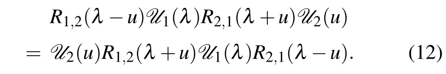
Now we introduce the double-row monodromy matrixU0(u)

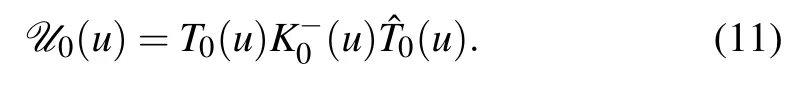
It can be demonstrated thatU0(u)also satisfies the RE

The corresponding transfer matrix is given by

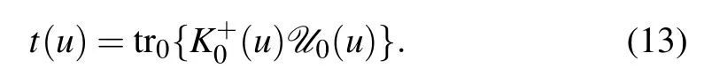
Using the crossing symmetry(2),(10)of theR-matrix and the reflection matrices,we can get

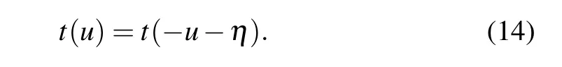
The QYBE and REs lead to that the transfer matrices with different spectral parameters commute mutually, i.e.,[t(u),t(v)]=0,which ensures the integrability of model(15).Therefore, the transfer matrixt(u) is the generating function of all the conserved quantities of the system.

The Hamiltonian of the quantumXXXspin-1/2 chain(or Heisenberg chain)with arbitrary boundary fields is given by

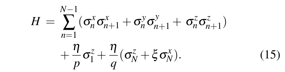
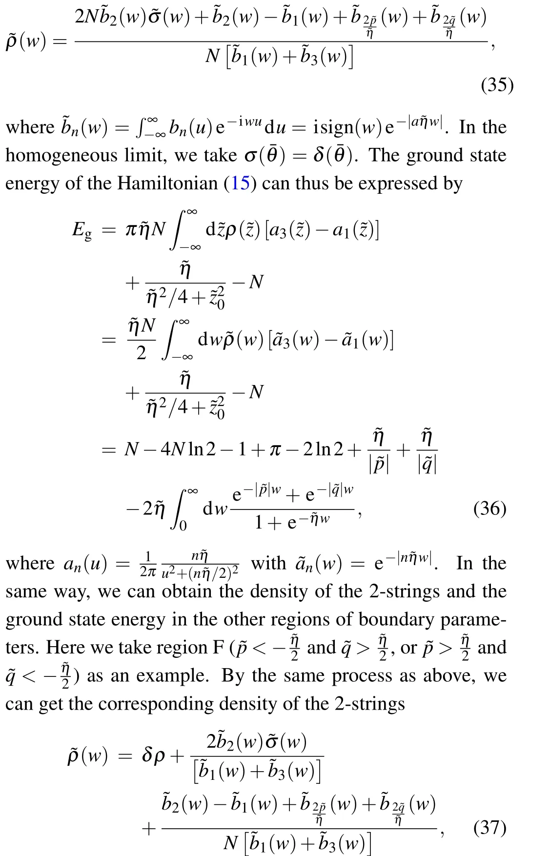
Combining Eqs.(13)and(15),the above Hamiltonian can be expressed by

For imaginaryη,to ensure a Hermitian Hamiltonian(15),the boundary parameters should be taken as follows:

For subsequent convenience,we define

Using the properties of theR-matrix (2), we can obtain the following operator identities:

where

From the definition(13)), we know that the transfer matrixt(u) is a polynomial operator ofuwith degree 2N+2.Denote the eigenvalue of the transfer matrixt(u)asΛ(u).

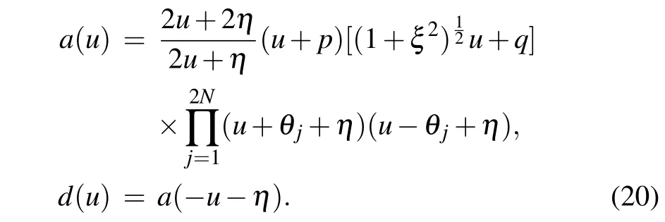
Combining Eqs.(13),(14)and(18),the eigenvalueΛ(u)satisfies

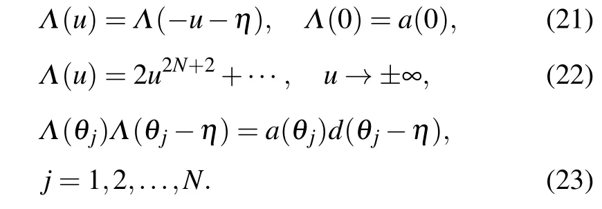
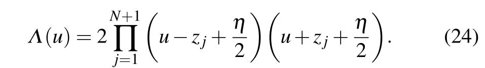
Therefore, for a given set of inhomogeneity parameters,Eqs. (21)–(23) can determine the roots{zj|j=1,...,N+1}completely. Now we can parameterize the eigenvalueΛ(u)by its rootszjas In the homogeneous limit{θj=0|j=1,...,N},Eq.(23)can be replaced by[17]

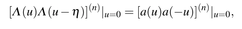
where the superscript (n) indicates then-th order derivative andn=0,1,...,N-1.

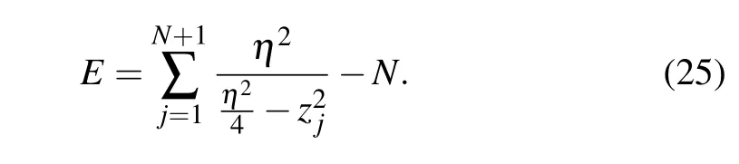
The eigenvalue of Hamiltonian(15)now can be expressed in terms of zero roots{zj|j=1,...,N+1}as follows:

3. Diagonal boundary case

For the diagonal boundary case(ξ=0), the constrained equations(21)and(23)become

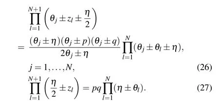
The aboveN+1 equations determineN+1 zeros totally. To give the patterns of zero roots, it is necessary to analyse the distribution of the Bethe roots.

3.1. Patterns of zero roots

Relations(1)and(7)imply that

Combining the imaginary{θj|j=1,...,N},we can get a hermitian transfer matrix

Combining Eqs.(24)and(29),we know that ifzjis a root ofΛ(u),thenmust be the root.

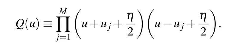
Firstly, we consider the parallel boundary case (ξ=0).We try to give all possible patterns of the zero roots with the help of the Bethe roots. It is known that the eigenvalue of transfer matrix(13)can be expressed by[18]

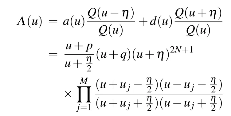
where

The corresponding Bethe ansatz equation can be written as

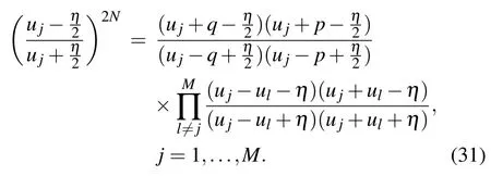
In the thermodynamic,the Bethe roots are real or form string structures{Im(ul) =ηn/2|n= 0,±1,±2...}.[21]Ifujis a Bethe root, thenmust also be a Bethe root. Combining Eqs. (24) and (30) atu=zj-η/2, we can also find that the zero roots satisfy the Bethe-ansatz-like equations

The above equation shows that the zero roots are constrained by the Bethe roots.

3.1.1. Bulk string

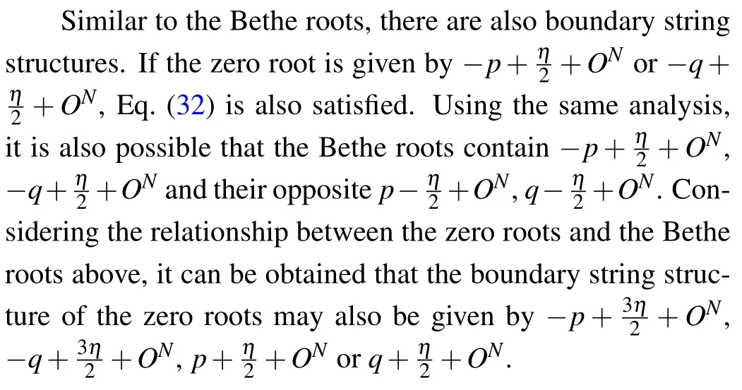
Equation (32) shows that for Im(zj)＞0, ifulis one of the Bethe roots, then±ul+ηis the corresponding zero roots. Considering{Im(ul) =ηn/2|n= 0,±1,±2...}, the imaginary parts of the zero roots can be written as{Im(zl)=ηn/2|n=0,±1,±2,±3...}.

However, forn=1 (uj=α-η/2), the corresponding zero root iszp=α+η/2. This configuration is actually impossible, because=α+η/2 is also a Bethe root, and the zero roots cannot be equal to the Bethe roots, which meanszp/=uj.[17]This is because if we define

forzp=uj,F(u) is the 2-degree zero point atuj, it requires an additional derivative equation of the BAEs. In this case,the BAEs are overdetermined, so we cannot give general solutions. Foruj=α-η/2, by considering the singularity of Eq. (32), we can give the correct zero roots. Supposing Im(zj)＜0, together with a similar analysis, we can obtain that the corresponding zero root iszp=α-3η/2.

With the above analysis, we conclude that the imaginary parts of the zero roots for the bulk string are{Im(zl)=ηn/2|n=0,±2,±3...}.

3.1.2. Boundary string

3.1.3. Additional roots

Besides these regular zero roots,we should note that there are additional roots, which means that a conjugate pair with imaginary parts neither around±ηn/2 (n ≥2) nor having a simple relation with boundary parameters. These roots are closely related with Eq. (21) and distributed at the boundary of the bulk string. They appear in two cases: (i) they appear symmetrically as pure real roots on the left and right sides of the bulk string and they tend to infinity in the thermodynamic limit; (ii) they appear symmetrically as pure imaginary roots on the upper and lower sides of the bulk string and they have no simple relation with the boundary parameters. Since the energy-related conclusions obtained afterwards are not related to them, we name them here as additional roots for convenience.

In summary, the possible structures of the zero roots are the combination of the bulk string,boundary string and the additional roots. Once we fix the structure of the bulk string and boundary string,the additional roots can be fixed by Eqs.(26)and(27)easily. In the next section,we will show that by solving Eq.(26)we can obtain the relation between the density of zero roots for the bulk string and the additional roots related to. Then jointly with Eq.(27)we can obtain another condition that constrains the additional roots to determine the relation between the additional roots and the boundary field parameters. In Fig. 1, we give some numerical results of the distributions of the Bethe roots and zero roots for large system size(N=100) at different parameter regions in the ground state.Moreover we can show that the possible structures of zero roots are exactly the same as that we have discussed above.Next we will study the structures of zero roots meticulously for the ground state.

Fig.1. Some numerical results of the distributions of the Bethe roots and zero roots on the complex plane for large system size(N=100)in the ground state. (a)and(c)The Bethe roots of the ground state corresponding to the select boundary parameters,respectively. (b)and(d)The zero roots of the ground state,respectively.

3.2. Ground state energy

A plausible fact is that by choosing a tunable set of nonzero inhomogeneity parameters, we can find that the zero root distributions show stable patterns. For imaginaryη, we choose all{θj}≡{i¯θj}to be imaginary. As shown in Fig.2,we adjust the distribution of the inhomogeneity parameters{θj}from the all-zero case to the non-zero case while the boundary field parametersp,q,ξare fixed. And we find that the zero roots for the bulk string keep a stable 2-strings structure with the introduce of this set of non-zero inhomogeneity parameters,while the real parts of these roots change slightly.By using the Fourier transformation of the auxiliary functionσ(¯θ), a density of the given inhomogeneity, the distribution of the zero roots of this inhomogeneous system along the 2-strings allows us to derive the density of the zero roots for the bulk string of the corresponding homogeneous system. The density of zero roots for the bulk string of the corresponding homogeneous system can then be obtained by taking the homogeneous limitσ(¯θ)→δ(¯θ). And the corresponding homogeneous system is exactly the model we consider.

In summary,in Fig.3 and Table 1 we give the phase diagram of the configuration of the zero roots for the ground state in different boundary parameter. We should note that there is always a pair of special additional zero roots constrained by Eq. (21). In the following parts, we will show that the unknown pair roots related to ˜zxwill not appear in the final result of energy.

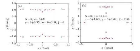
Fig.2. Exact numerical diagonalization results of the zero root distributions in the ground state for N =8. (a) The red asterisks indicate¯z-roots for {¯θj =0|j=1,...,N} and the blue circles specify the zero roots with the inhomogeneity parameters {¯θj =0.05 j|j=1,...,N}.(b)The red asterisks indicate the zero roots for{¯θj =0|j=1,...,N}and the blue circles specify ¯z-roots with the inhomogeneity parameters{¯θj =0.1j|j=1,...,N}.

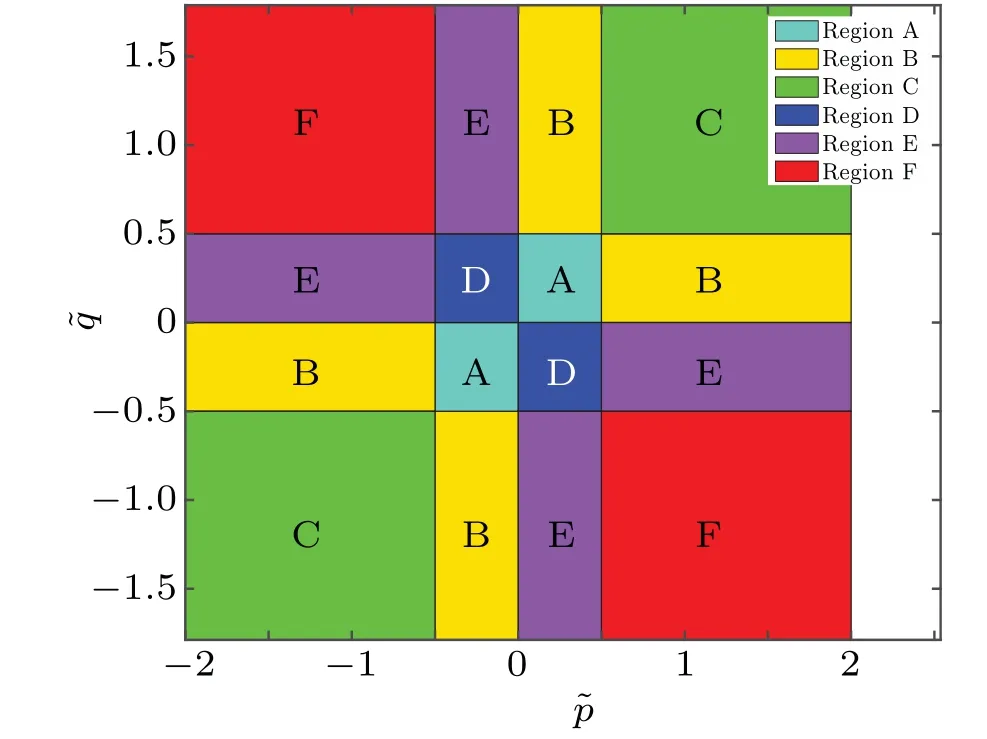
Fig.3. The phase diagram of the configuration of the zero roots for the ground state in the different regions of boundary parameters ˜p and ˜q with ˜η =1.

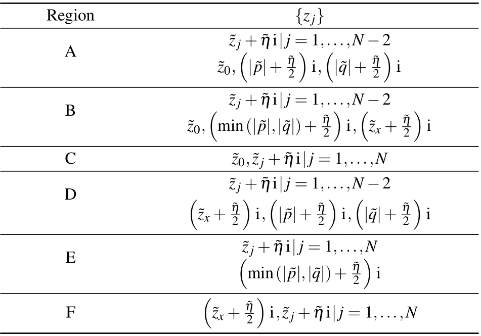
Table 1. The patterns of zero roots for the ground state in different regions,where the roots related to ˜z0 or ˜zx are the additional roots,the roots related to ˜zj are the the bulk string, ˜z0 is a real number greater than the maximum value in{˜zj}and ˜zx is a real number greater than ˜η/2,and{˜zj}are all real.

where

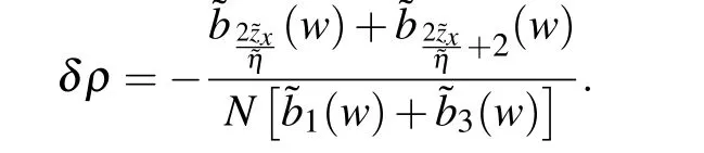
So the ground state energy in region F can be written as

We find that the appearance of the pure imaginary additional roots changes the 2-strings density byδρ,but the energy change caused byδρand the contribution of the additional roots itself cancel each other out exactly. Thus, the ground state energy of region F is equal to that given by Eq. (36).Combining Eq.(37),the specific value of the pair of additional roots related tocan be constrained by Eq. (27) in the thermodynamic limit as

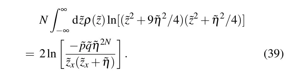
Through numerical analysis,we find that this pair of additional roots related todoes not change with the number of sitesN.As for other parameter regions, the calculation is exactly the same. Finally,we conclude that the ground state energy for all parameter regions has the same expression as Eq. (36). The result shows that the contributions of the two boundary fields to the surface energy are additive.

4. Off-diagonal boundary case

The constrained equations(21)and(23)become

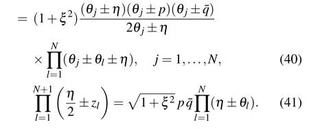
The only difference between the constrain equations(40),(41)and(26),(27)is a constant coefficient.

4.1. Surface energy

Through the previous discussion,we can find that in this case the boundary parameterplays the same role withqin the diagonal boundary case. We can guess that this similarity also existed in the distributions of zero roots for the ground state. The numerical results for the distributions in this case coincide with this guess. In Fig.4,we give some numerical result of the distribution form forN=10 at different parameter regions for the ground state.

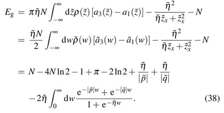
Through the same numerical method and derivation process in theξ/=0 case, we can get the patterns of zero roots corresponding to the ground state with different boundary parameter regions as shown in Fig.3 and Table 1 which take ˜pas the horizontal axis and ˆqas the vertical axis in this case, and the ground state energy takes

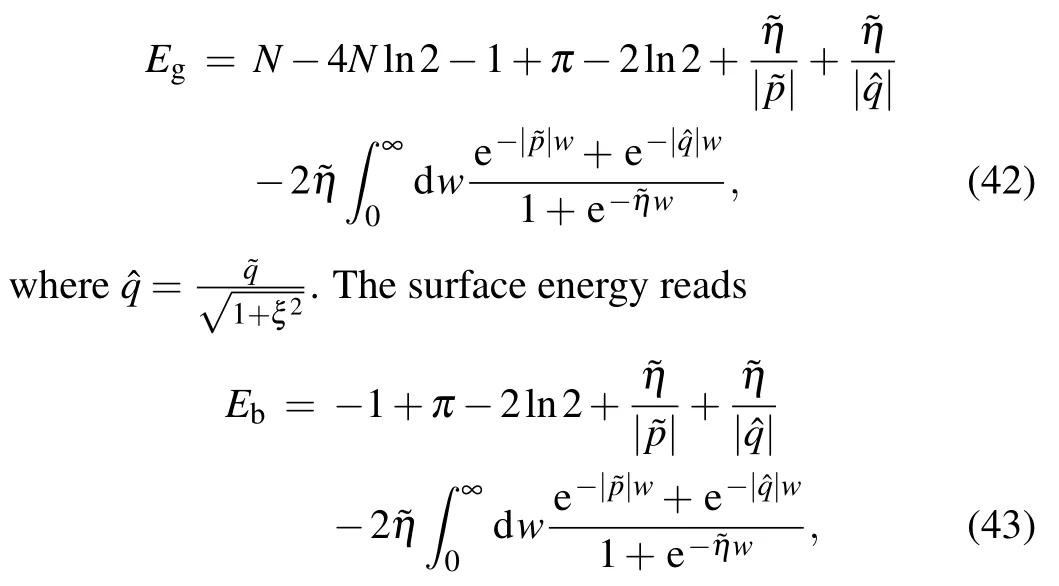
which is defined byEb=Eg-Ep,whereEgis the ground state energy of the present system andEpis the ground state energy of the corresponding periodic chain.[14]This result indicates that the contributions of the two boundaries to the surface energy are also additive in this case. The DMRG results and our analytic results are shown in Figs.5 and 6. The present result also coincides exactly with that derived in Ref[24].

Fig.5. Our analytic results of the surface energy for η =1i,ξ =0.

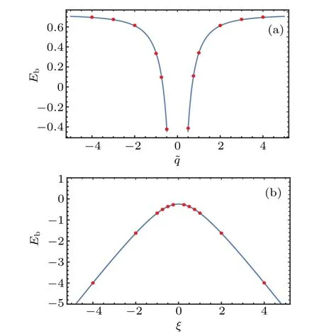
Fig.6. Comparison of the DMRG results and our analytic results of the surface energy. (a) The DMRG results for N =200 expressed by the red points and our analytic results expressed by the curve for η =1i,p=-4i,ξ =0. (b)The DMRG results for N=200 expressed by the red points and our analytic results expressed by the curve for η =1i,p=1i,q=-0.75i.

Through the previous analysis of the structure of zero roots, it can be found that the distribution of zero roots on the complex plane can be divided into several categories. By performing different kinds of fine-tuning on the zero roots distribution of the eigenvalue of the transfer matrix corresponding to the ground state,the zero roots distribution of the eigenvalue of the transfer matrix corresponding to the low-energy excited state can be found,and then several possible excitations can be calculated. At the same time,we also verified the existence of the guessed low-energy excited state through numerical analysis. Here we summarize some kinds of excitations.

4.1.1. Elementary excitation 1

Comparing with the zero roots distribution of the eigenvalue of the transfer matrix corresponding to the ground state,the two pairs of conjugate pairs{,}will disappear in the zero roots distribution of the eigenvalue of the transfer matrix corresponding to the first kind of low-energy excited state shown in Fig. 7, and two pairs of real numbers{}will appear.For real numbers,the resulting change in the density of the 2-strings is

The energy of the corresponding excitation is

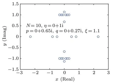
Fig.7. The distribution of zero roots at a low-lying excited state of type 1 corresponding to the ground state in Fig.4(a).

4.1.2. Elementary excitation 2

The energy of the corresponding excitation is

In the same way, the excitations caused by the change of the boundary string related topcan be obtained.

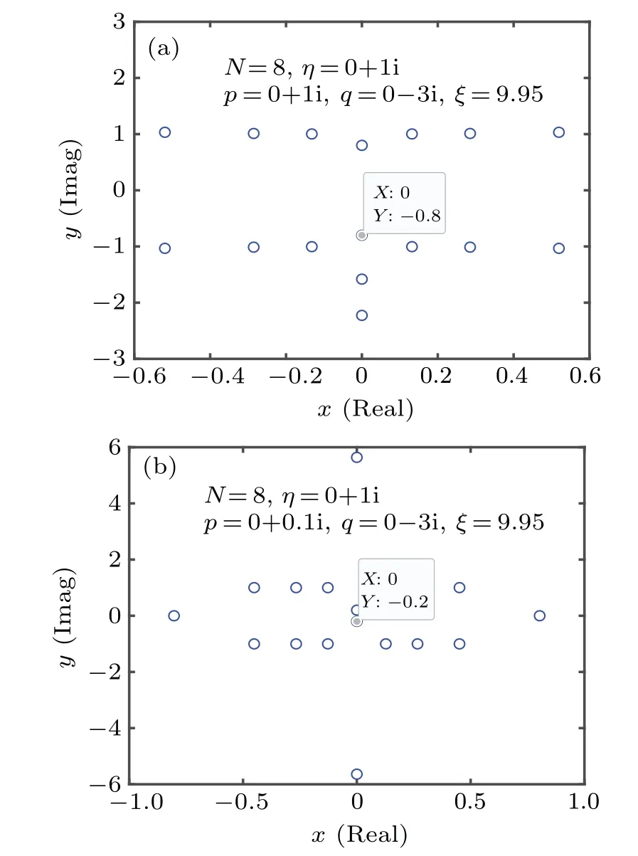
Fig.8. (a)The distributions of zero roots for the ground state with the parameters N=8, ˜η=1, ˜p=1, ˜q=-3,ξ =9.95 and ˆq=0.3. (b)The distributions of zero roots for the corresponding low-lying excited state of type 2.

In addition, compared with the zero roots distribution of the eigenvalue of the transfer matrix corresponding to the ground state and the zero roots distribution of the eigenvalue of the transfer matrix corresponding to other low-energy excited states,two pairs of conjugate pairs{,}may transition to the higher 2-strings and become{,}, wherenis an integer greater than 2, or transition on the imaginary axis and become{)i,±(+}. When the number of sites in the model is limited,we find the energy of these kinds of excitations is not zero through numerical analysis. But in the thermodynamic limit,the energy of excitations of these types is zero.

5. Conclusion

We obtain the surface energy and elementary excitations of theXXXspin-1/2 chain with arbitrary non-diagonal boundary fields through a combination of numerical analysis and analytical derivation. Firstly, through the analysis of the BAEs(32),the general patterns of zero roots of eigenvalue of the transfer matrix are obtained in Section 3.Then by using the numerical analysis,the zero roots structure of the ground state and various low-energy excited states are determined. Finally,the zero roots density is determined by the relations(23)satisfied by the eigenvalue of the transfer matrix,while the surface energy and elementary excitations of the model are solved in the thermodynamic limit. The method used here can be generalized to other integrable models solved via the off-diagonal Bethe ansatz.[17,27–30]

Acknowledgements

We would like to thank Professor Y. Wang for his valuable discussions and continuous encouragement. The financial supports from the National Key R＆D Program of China(Grant No. 2021YFA1402104), the National Natural Science Foundation of China (Grant Nos. 12074410, 12047502,12147160, 11934015, 11975183, and 11947301), Major Basic Research Program of Natural Science of Shaanxi Province,China (Grant Nos. 2021JCW-19 and 2017ZDJC-32), Strategic Priority Research Program of the Chinese Academy of Sciences(Grant No.XDB33000000),Double First-Class University Construction Project of Northwest University,and the fellowship of China Postdoctoral Science Foundation (Grant Nos. 2020M680724 and 2022M712580) are gratefully acknowledged.