The coupled deep neural networks for coupling of the Stokes and Darcy–Forchheimer problems

Jing Yue(岳靖), Jian Li(李剑),†, Wen Zhang(张文), and Zhangxin Chen(陈掌星)

1School of Electrical and Control Engineering,School of Mathematics and Data Science,Shaanxi University of Science and Technology,Xi’an 710021,China

2School of Mathematics and Statistics,Xi’an Jiaotong University,Xi’an 710049,China

3Department of Chemical and Petroleum Engineering,Schulich School of Engineering,University of Calgary,2500 University Drive N.W.,Calgary,Alberta T2N 1N4,Canada

Keywords: scientific computing, machine learning, the Stokes equations, Darcy–Forchheimer problems,Beavers–Joseph–Saffman interface condition

1. Introduction

Fluid flows between porous media and free-flow zones have extensive applications in hydrology, environmental science, and biofluid dynamics. A lot of researchers have derived suitable mathematical and numerical models for fluid movement.[1–3]A system can be viewed as a coupled problem with two physical systems interacting across an interface.The simplest mathematical formulation for the coupled problem is coupling of the Stokes and Darcy flow with proper interface conditions. The most suitable and popular interface conditions are called the Beavers–Joseph–Saffman conditions.[4]However, Darcy’s law only provides a linear relationship between the gradient of pressure and velocity in the coupled model, which usually fails for complex physical problems.Forchheimer[5]conducted flow experiments in sand packs and recognized that for moderate Reynolds numbers(Re ＞0.1 approximately), Darcy’s law is not adequate. He found that the pressure gradient and Darcy velocity should satisfy the Darcy–Forchheimer law. Since the great attention has been paid to the coupled model, a large number of traditional mesh-based methods have been devoted to the coupled Stokes and Darcy flows problems.[6–22]

Owing to the enormous potential in approximating complex nonlinear maps,[26–32]deep learning has attracted growing attention in many applications, such as image, speech,text recognition,and scientific computing.[23–25]Many works have arisen based on the function approximation capabilities of the feed-forward fully connected neural network to solve initial/boundary value problems[40–43]in recent decades. The solution to the system of equations can be obtained by minimizing the loss function,which typically consists of the residual error of the governing partial differential equations(PDEs)along with initial/boundary values. Resently,Raissiet al. proposed physics informed neural networks (PINNs)[44–46]and they have been widely used.[47–52]Moreover, Sirignano and Spiliopoulos presented the deep learning Galerkin method[54]for solving high dimensional PDEs. Additionally,some recent works have successfully solved the second-order linear elliptic equations and the high dimensional Stokes problems.[33–36]Though several excellent works have been performed in applying deep learning to solve PDEs,[37]the topic for solving complicated coupled physical problems remains to be investigated.

Considering the performance of deep learning for solving PDEs,our contribution is to design the CDNNs as an efficient alternative model for complicated coupled physical problems.We can encode any underlying physical laws naturally as prior information to obey the law of physics. To satisfy the differential operators, boundary conditions and divergence conditions, we train the neural networks on batches of randomly sampled points. The method only inputs random sampling spatial coordinates without considering the nature of samples.Notably,we take the interface conditions as the constraint for the CDNNs.The approach is parallel and solves multiple variables independently at the same time. Specially, the optimal solution can be obtained by using the networks instead of a linear combination of basic functions. Furthermore,we validate the convergence of the loss function under certain conditions and the convergence of the CDNNs to the exact solution. Several numerical experiments are conducted to investigate the performance of the CDNNs.

The article is organized as follows: Section 2 introduces the coupled model and the relation methodology. Section 3 discusses the convergence of the loss functionJ() and the convergence of the CDNNs to the exact solution. Section 4 reveals some numerical experiments to illustrate the efficiency of the CDNNs. The article ends with conclusion in Section 5.

2. Methodology

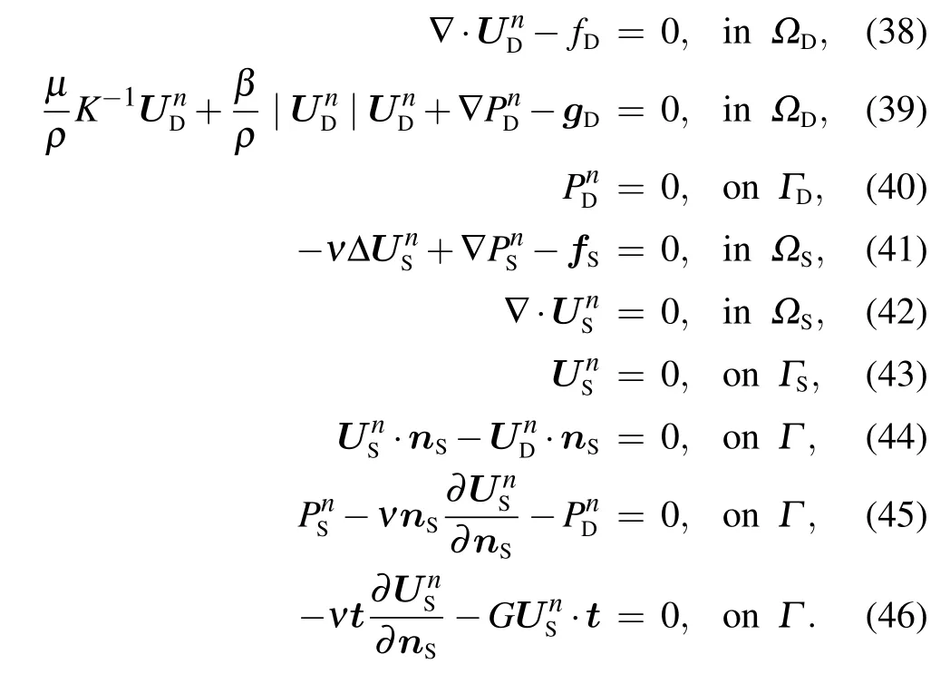
LetΩSandΩDbe two bounded and simply connected polygonal domains in R2, as shown in Fig. 1. LetnSdenote the unit normal vector pointing fromΩStoΩD,and takenDas the unit normal vector pointing fromΩDtoΩS,on the interfaceΓ,then we havenD=-nS.

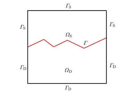
Fig.1. Coupled domain with interface Γ.

When kinematic effects surpass viscous effects in a porous medium, the Darcy velocityuDand the pressure gradient ∇pDdoes not satisfy a linear relation. Instead,a nonlinear approximation, known as the Darcy–Forchheimer model,is considered. When it is imposed on the porous mediumΩDwith homogeneous Dircihlet boundary condition onΓD, the equations can be written as

whereKis the permeability tensor assumed to be uniformly positive definite and bounded,ρis the density of the fluid,μis viscosity,andβis a dynamic viscosity,all assumed to be positive constants. In addition,gDandfDare source terms. We remark that in this context we exploit homogeneous Dirichlet boundary condition,in fact,we can also consider homogeneous Neumann boundary condition, i.e.,uD·nD=0 onΓDand the arguments used in this paper are still true.

The fluid motion inΩSis described by the Stokes equations:

whereν ＞0 denotes the viscosity of the fluid.

On the interface, we prescribe the following interface conditions:

Here,trepresents the unit tangential vector along the interfaceΓ. Condition(7)represents continuity of the fluid velocity’s normal components,Eq.(8)represents the balance of forces acting across the interface,and Eq.(9)is the Beavers–Joseph–Saffman condition.[55]The constantG ＞0 is given and usually obtained from experimental data.

For notational brevity,we set=(uS,uD,pS,pD)and recall the classical Sobolev spaces

where

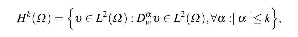
and their norm

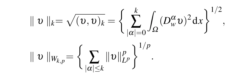
Particularly,‖v‖k=‖v‖Wk,2. Here,k ＞0 is a positive integer,‖υ ‖0denotes the norm onL2(Ω) or (L2(Ω))2, andDαwυis the generalized derivative ofυ. Moreover,(·,·)Drepresents the inner product in the domainDand〈·,·〉represents the inner product on the interfaceΓ.

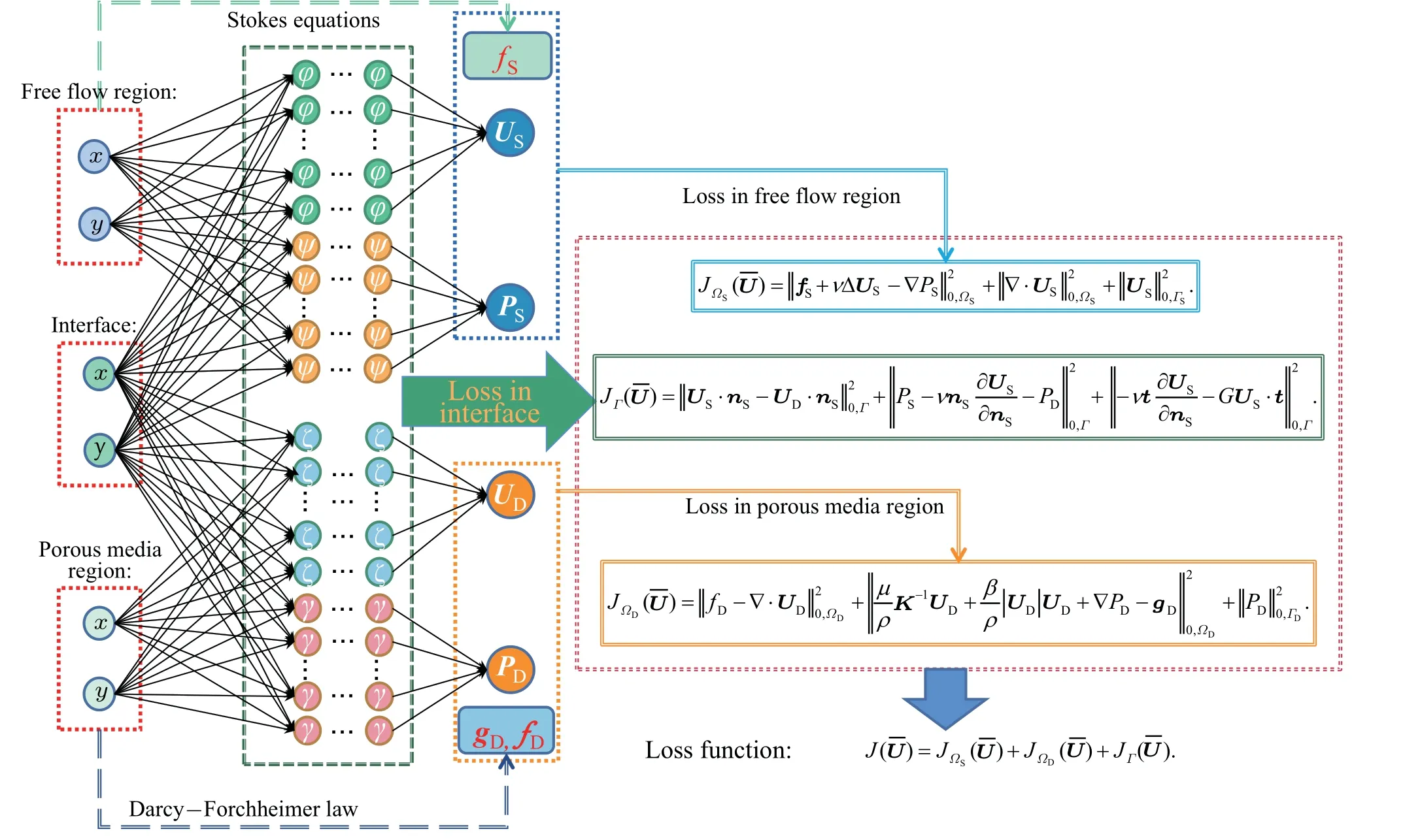
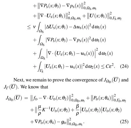
Fig.2. The structure of the CDNNs.

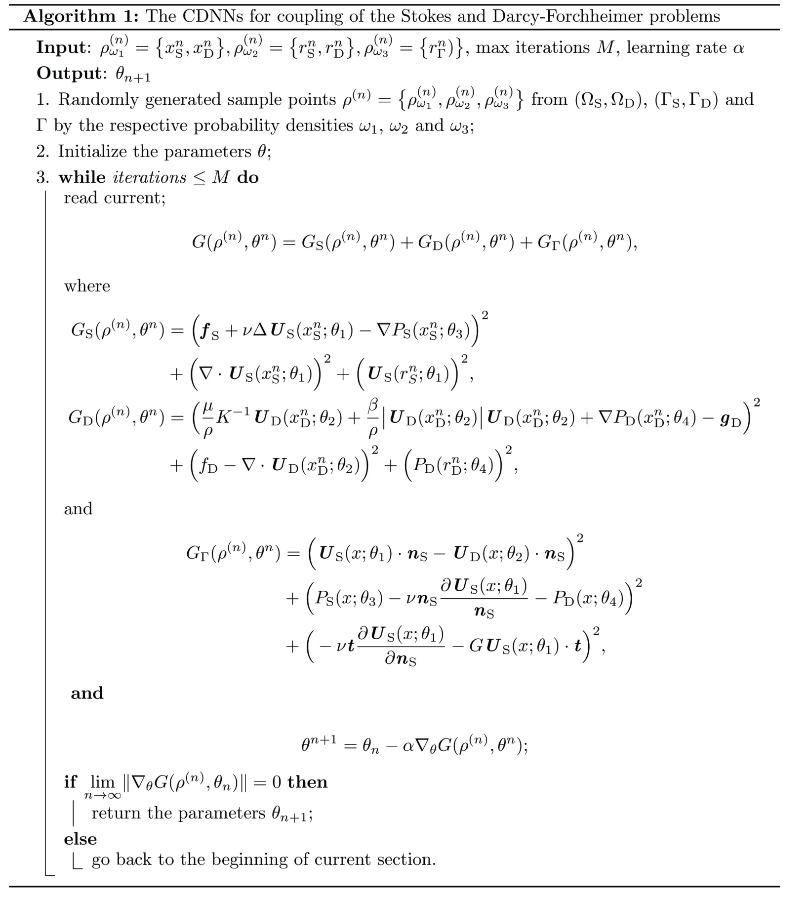
To solve coupling of the Stokes and Darcy–Forchheimer problems, we propose the CDNNs in Fig. 2, wherex,yrepresent the spatial coordinates in different domains. Furthermore, we give observations of the state variable(x;θ) =（US(x;θ1),UD(x;θ2),PS(x;θ3),PD(x;θ4)）, which is the neural network solution to the coupled Stokes and Darcy–Forchheimer problems (1)–(9). Here, (θ1,θ3) and (θ2,θ4)are the stacked parameters ofθfor Stokes and Darcy–Forchheimer, respectively. The following constrained optimization procedure aims to reconstruct the parametersθby minimizing the loss function:

where

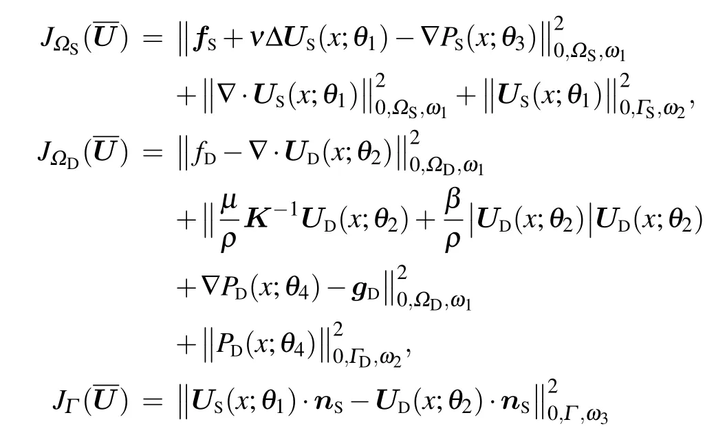
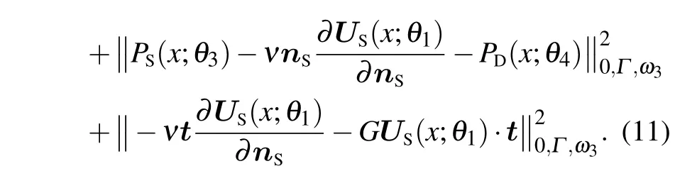
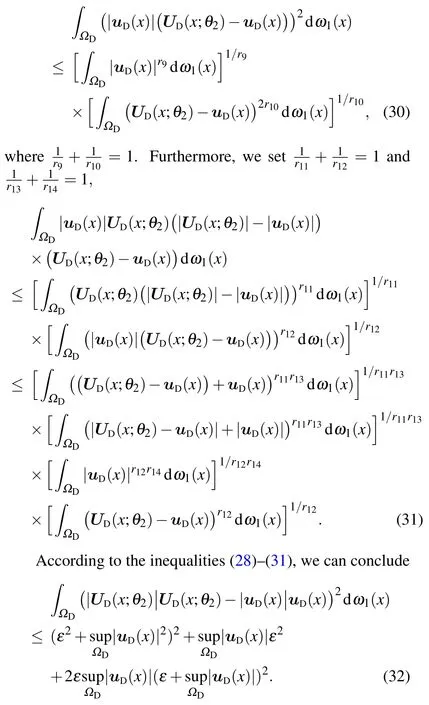
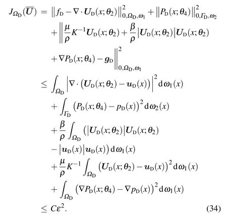
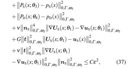
It should be noted thatJ(U)can measure how well the approximate solution satisfies differential operators, divergence conditions,boundary conditions and interface conditions.Furthermore, the norm in Eq. (11) means thaty,ω=ω(y)dy, whereω(y) is the probability density of variableyin domainY. In this study, the training data are sampled randomly from interior domains, boundary domains and interface by the respective probability densitiesω1,ω2,andω3. Especially, ifJ()=0, thenis the solution to the coupled Stokes and Darcy–Forchheimer problems(1)–(9).Since it is infeasible to estimateθby directly minimizingJ() when integrated over a higher dimensional region, we apply a sequence of randomly sampled points from domain instead forming mesh grid. The main steps of the CDNNs for the coupled Stokes and Darcy–Forchheimer equations are presented as Algorithm 1. Another noticeable point is that the term ∇θG(ρ(n),θn)is unbiased estimate of ∇θJ（(·;θn)）because the population parameters can be estimated by sample mathematical expectations.

3. Convergence

According to the defniition of loss functionJ(), it can measure how wellsatisfeis Eqs. (1)–(9). Neural networks are a set of algorithms for classification and regression tasks inspired by the biological neural networks in brains. There have various types of neural networks with different neuron connection forms and architectures. According to Ref.[29],if there is only one hidden layer and output,a set of functions implemented by following networks withm1,m2,m3andm4hidden units for coupling of the Stokes and Darcy–Forchheimer problems are

More generally,we use the similar notation

for the multi layer neural networks with arbitrarily large number of hidden unitsm1,m2,m3andm4. In particular, the parameters and the activation function in each dimension of[(φ)]dor [(ζ)]dare same as before. For convenient,we setnas the number of the neurons in numerical experiments. Then the parameters of the CDNNs can be formalized as follows:

wherek= 1,2,...,d,θ1∈R(2+d)nd,θ2∈R(2+d)nd,θ3∈R(2+d)n,andθ4∈R(2+d)n.

3.1. Convergence of the loss function J()

In this subsection,we prove that the CDNNsUcan make the loss functionJ()arbitrarily small.

Assumption 1∇v(x),Δv(x) and ∇q(x) are locally Lipschitz with Lipschitz coefficient such that they have at most polynomial growth onv(x) andq(x). Then, for some constants 0≤qi ≤∞(i=1,2,...,6)we have

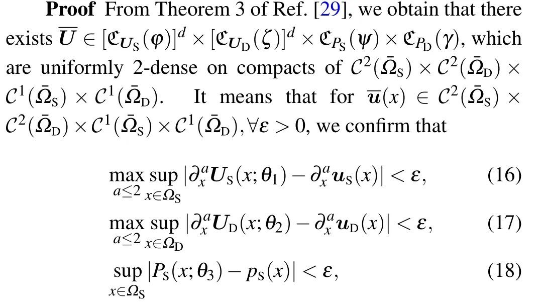
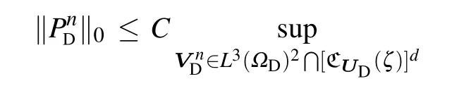
Theorem 1Under Assumption 1, there exists a neural network∈[CUS(φ)]d×[CUD(ζ)]d×CPS(ψ)×CPD(γ),satisfying

whereCdepends on the data{ΩS,ΩD,Γ,μ,ρ,β,K-1,ω1,ω2,ω3,fD,gD,fS}.

Firstly, we recall the form and discuss the convergence ofJΩS∖Γ(),

Here we setl1∨l2=max{l1,l2}. In the same way,

For the boundary condition,we have

Owing to Eqs.(21)–(23),we conclude that

From Eq.(19),we have

which can be updated by using the H¨older inequality and Young inequality,thus we have

by using the H¨older inequality and Young inequality, setting conjugate numbersr7andr8such that=1.

Similarly,we can obtain

For the boundary condition,we know

Combining Eqs.(26)–(33),we obtain

The loss in interface is referred in Eq.(11). According to Assumption 3.1,we know

which can be updated by using the H¨older inequality and Young inequality,thus we have

which completes the proof.

3.2. Convergence of the CDNNs to the exact solution

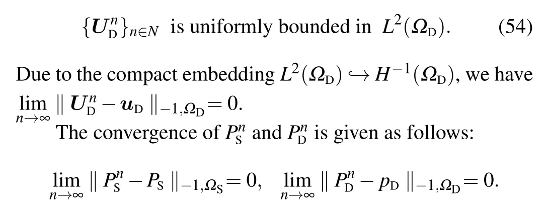
In the above subsection,we have proved the convergence of the loss function. In this subsection, we remain to discuss the convergence of the CDNNs to the exact solution. According to the Galerkin method,the neural networks satisfy

Based on the above system of equations,we give the following assumption and theorem to guarantee the convergency of the CDNNs to the exact solution.

Considering the interface conditions, simple algebraic calculation yields

which,by employing interface conditions(45)and(46),gives

For convenience of presentation,we introduce the nonlinear operatorA:L3(ΩD)2→L3/2(ΩD)2defined by

The definition of Eq.(52)gives

According to Assumption 2 and Eq.(50),

According to the definition of theH1norm, the Young inequality and the Poincar´e inequality,we can obtain

Thus we have

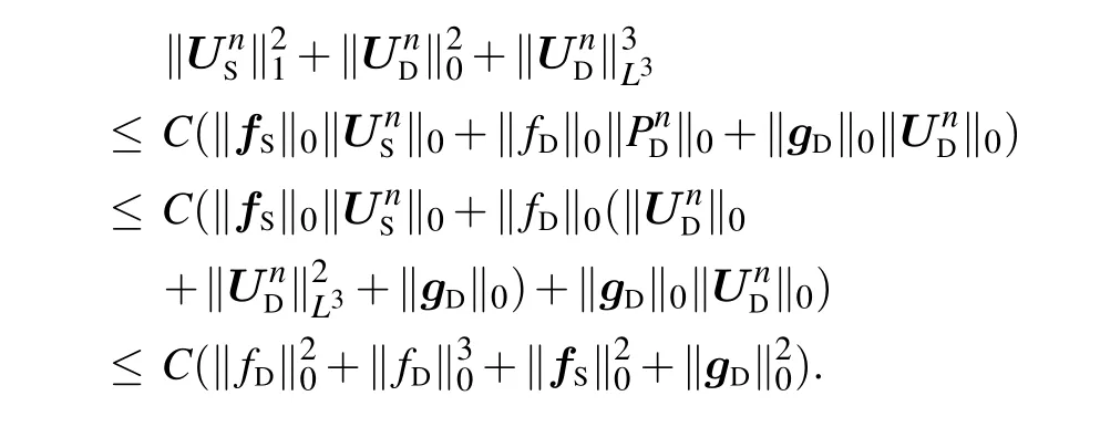
According to Assumption 2,Eqs.(47)–(48)and Eq.(51),we have

Up to now,we obtain:

Similarly,we knowL3(ΩD)⊂L2(ΩD),which implies that

4. Numerical experiments

The section presents several numerical tests to confirm the proposed theoretical results. We start with three examples with known exact solution to test the efficiency of the proposed method,where the permeability for the third example is highly oscillatory. Then, the fourth example with no exact solution shows the application of the proposed method to high contrast permeability problem. This section concludes with a physical flow. The numerical examples presented could violate the interface conditions (8) and (9),[56]that is, Eqs. (8) and (9) are replaced by Eqs.(55)and(56)to deal with this case,

the variational formulation has only a small change: Eq.(51)now includes the two terms-〈g1,VS·nS〉Γ-〈g2,VS·t〉Γon the right side. In addition, we utilize 16 neurons in each hidden layer and apply the relativeL1error(errL1:)and relativeL2error (errL2:)to reflect the accuracy between the results of the CDNNs and the exact solution(r: the exact solution;R: the neural network).

4.1. Test 1

In this subsection we study the performance of the CDNNs for the benchmark problem presented in Ref. [56].This problem is defined forΩS=(0,1)2,ΩD=(0,1)×(1,2)and the interfaceΓ={0＜x ＜1,y=1}as

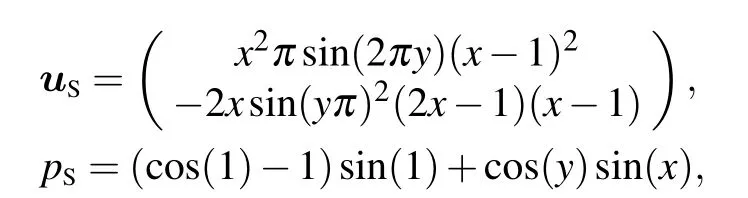
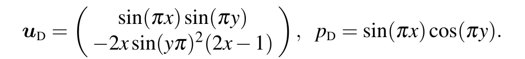
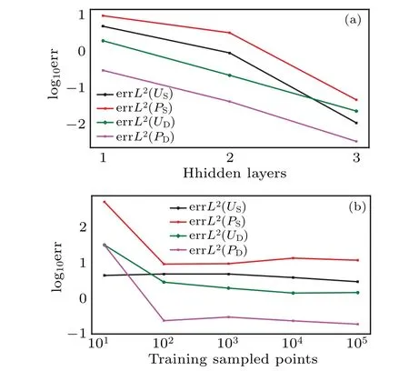
Fig.3. The influence of different hidden layers and different training data on err L2 (Test 1): (a)400 training points,(b)one hidden layer.

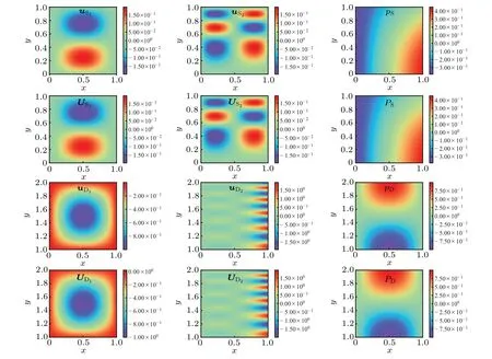
Fig.4. The contrast of the exact solution and the CDNNs(Test 1).

Similar to Ref.[56],we fixKto be the identity tensor in R2×2,μ=ρ=β=ν=1. Due to the fact that the interface conditions (8) and (9) are violated, we exploit the interface conditions (55) and (56), whereg1andg2can be computed by the exact solution. Specifically, the errors converge as the hidden layer increases in Fig.3(a). Figure 3(b)reveals that the change of data has no significant influence on errors once the size is larger than 102. In particular,Fig.4 displays the exact solution of the couples Stokes Darcy–Forchheimer problems and the results of the CDNNs, one can observe that both are approximately identical. The point-wise errors are depicted in Fig. 5. As can be seen, the absolute errors are almost all 0,which also indicates the closeness between the exact solution and the approximation solution. Table 1 exhibits the details of the results,which are consistent with our theory.

Fig.5. The point-wise errors(Test 1).

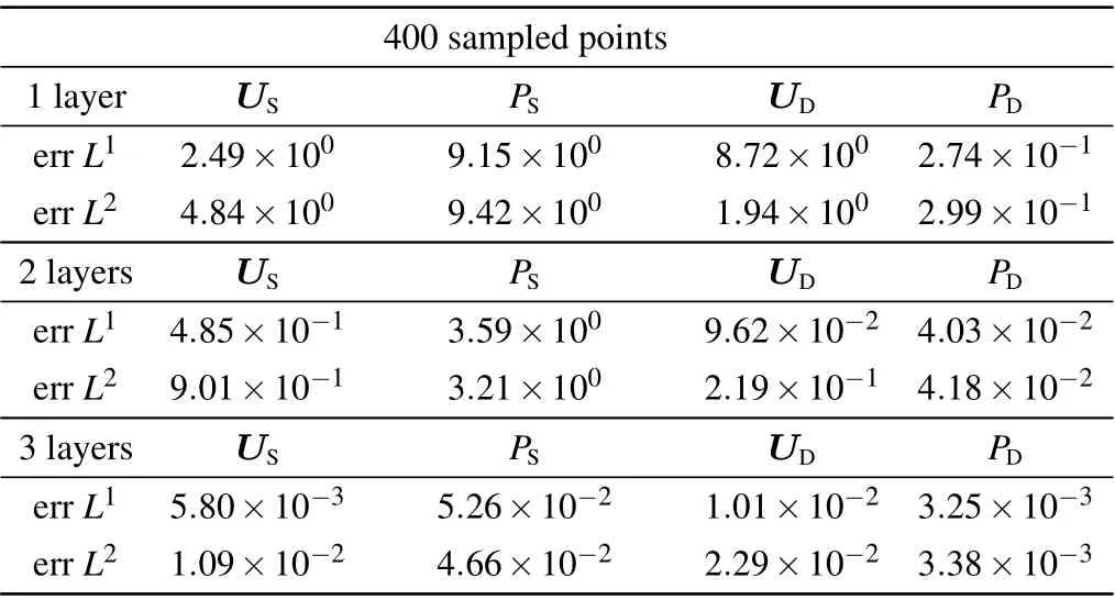
Table 1. The relative errors of Test 1.

4.2. Test 2

In this example,we considerΩS=(0,1)2,ΩD=(0,1)×(1,2) and the interfaceΓ={0＜x ＜1,y=1}with an analytical solution presented in Ref. [56]. We setKto be the identity tensor in R2×2,μ=ρ=β=ν=1, and the exact solution is given by

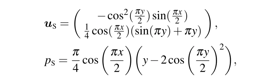
and

Naturally,the correspondingfS,fD,andgDcan be calculated by the exact solution. Note that this example satisfies the interface conditions (7)–(9). According to Test 1, we choose appropriate data and hidden layer to solve the second example. Figure 6 and Table 2 show the accuracy of the CDNNs for solving the coupled problems in detail.

Table 2. The relative errors of Test 2.

Fig.6. The point-wise errors(Test 2).

4.3. Test 3

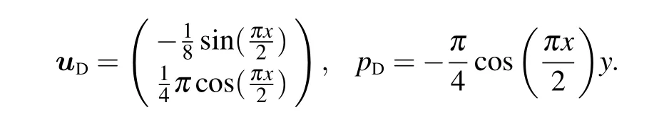
In this subsection, we solve coupling of the Stokes and Darcy–Forchheimer problems with highly oscillatory permeability over domainsΩS= (0,1)×(0,1/2),ΩD= (0,1)×(1/2,1)and the interfaceΓ={0＜x ＜1,y=1/2}presented in Ref.[56]. Here we setμ=ρ=β=ν=1,K-1=ρI,andρis defined by

whereε=1/16. The profile ofρis shown in the figure. The exact solution is given by

We calculate the relative errors in Table 3 to reflect ability of the CDNNs for solving the coupled problems with highly oscillatory permeability (Fig. 7). Figure 8 reveals that the CDNNs handle the highly oscillatory permeability coupled problems without losing accuracy.

4.4. Test 4

The problems that we have studied so far have the exact solution. In this example,we consider coupling of the Stokes and Darcy–Forchheimer problems with no exact solution overΩS=(-1/2,3/2)×(0,2),ΩD=(-1/2,3/2)×(-2,0) and the interfaceΓ={-1/2＜x ＜3/2,y=0}. Specifically, in the Stokes region,the Dirichlet boundary condition is given by Kovasznay flow,[57]

whereλ=Moreover,we setμ=ρ=β=ν=1 andgD=0,fD=0,fS=0.In addition,pDsatisfies the homogeneous Dirichlet boundary condition alongy=-2,otherwise it has an homogeneous Neumann boundary condition. The permeability is taken to beK=εIand theε=104. Since the exact solution for this example is unavailable, we provideL2error of interface to demonstrate the accuracy of the CDNNs in Table 4.Obviously,the error decreases gradually with increase of the hidden layers. Furthermore, Figs.9 and 10 display the exact solution and the results of CDNNs in detail.

Fig.7. The value of ρ (Test 3).

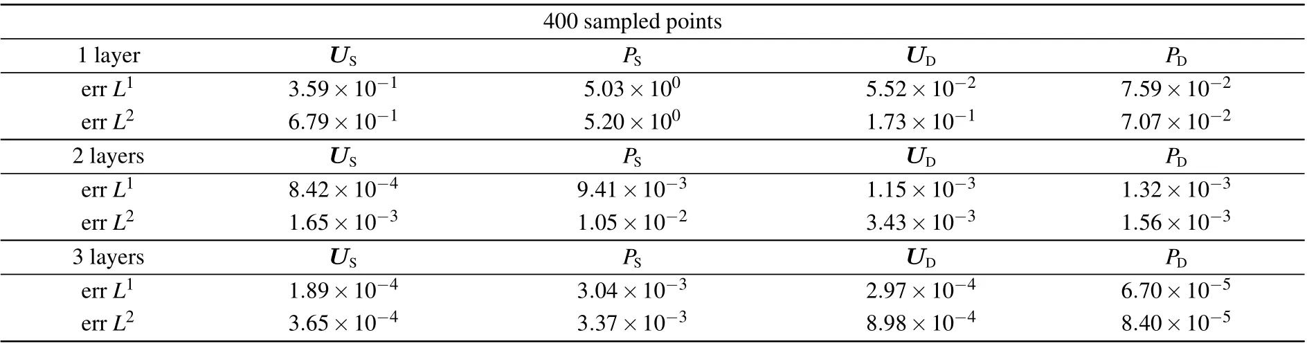
Table 3. The relative errors of Test 3.

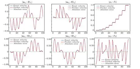
Fig.8. The point-wise errors(Test 3).

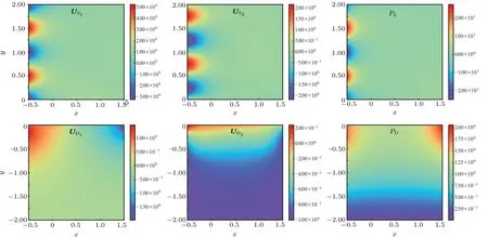
Fig.9. The results of CDNNs(Test 4).

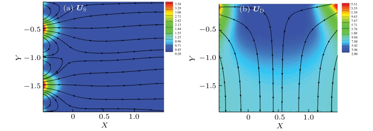
Fig.10. The velocity flows of Stokes and Darcy(Test 4).

Table 4. The errors in interface of Test 4(K=10000).

4.5. Test 5

We conclude this section with a physical flow, whereΩS=(0,1)×(1,2),ΩD=(0,1)2and the interfaceΓ={0＜x ＜1,y=1}. InΩS, the boundaries of the cavity are walls with no-slip condition, except for the upper boundary where a uniform tangential velocityuS(x,2) = (1,0)Tis imposed,which is driven cavity flow. More precisely, we enforce homogeneous Neumann and Dirichlet boundary conditions, respectively,onΓD,N={x=0 ory=0}andΓD,D={x=1}. In addition,we setKto be the identity tensor in R2×2,μ=ρ=β=ν=1, andfD=0,fS=0,gD=0. The results of the CDNNs are depicted in Fig.11. More vividly,we display the velocity flows of free-flow and porous media zones in Fig.12.

Fig.11. The results of the CDNNs(Test 5).

Fig.12. The velocity flows of Stokes and Darcy(Test 5).

5. Conclusions

In summary, we have proposed the CDNNs to study the coupled Stokes and Darcy–Forchheimer problems. Our method compiles the interface conditions of the coupled problems into the networks properly and can be served as an efficient alternative to the complex coupled problems. CDNNs avoid limitations of the traditional methods, such as decoupling, grid construction and the complicated interface conditions. Furthermore, it is meshfree and parallel, it can solve multiple variables independently at the same time. Specially,we provide the convergence of the loss function and the convergence of the CDNNs to the exact solution. The numerical results are consistent with our theory sufficiently. Moreover,we leave the following issues subject to our future works: (1)combining data-driven with model-driven to solve the high dimensional coupled problems, (2) considering the specific size of the networks through theoretical analysis,(3)combining traditional numerical methods with deep learning to solve more complicated high dimensional coupled problems.

Acknowledgements

Project supported in part by the National Natural Science Foundation of China (Grant No. 11771259), the Special Support Program to Develop Innovative Talents in the Region of Shaanxi Province, the Innovation Team on Computationally Efficient Numerical Methods Based on New Energy Problems in Shaanxi Province, and the Innovative Team Project of Shaanxi Provincial Department of Education(Grant No.21JP013).