Physics-based model for boundary layer transition prediction in a wide speed range

Zijie LIU， Yuhn LU， Sheng WANG， Qing WANG， Cho YAN，*

a School of Aeronautic Science and Engineering， Beihang University， Beijing 100083 China

b Research Institute of Navigation and Control Technology， Beijing 100089， China

c China Academy of Aerospace Aerodynamics， Beijing 100074， China

KEYWORDS Boundary layer;High-speed;Physics-based;Transition model;Transitional flow

Abstract A new physics-based model employing three transport equations is developed for the simulation of boundary layer transitions in a wide speed range. The laminar kinetic energy is used to represent pretransitional streamwise velocity fluctuations， taking account of different instability modes. The fluctuation velocity components normal to the streamwise direction are modeled by another transport equation. Transition is triggered automatically with the development of the pretransitional velocity fluctuations. In the fully turbulent region， the model reverts to the k-ω turbulence model. Different test cases， including subsonic， supersonic and hypersonic flows around flat plates， airfoils and straight cones， are numerically simulated to validate the performance of the model. The results demonstrate the excellent predictive capabilities of the model in different paths of transition.The model can serve as a basis for the extension of additional transition mechanisms，such as rotation and curvature effects， roughness-induced transition and crossflow-induced transition.

1. Introduction

Laminar-turbulence transition is a common occurrence in a wide range of industrial systems，including，for example，those in aeronautics， astronautics， wind turbines and power generation. Generally， transition is accompanied by remarkable growths in frictional drag and the aerothermal environment.Thus， accurate prediction of transitional flows is of vital importance in the design of aerodynamic configurations and thermal protection systems. However， it is difficult to predict transition accurately， because its inherent behavior is complex and not fully understood， and the transition process is influenced by various parameters such as freestream turbulence levels， pressure gradients， Reynolds number， Mach number and roughness. This wide variety of factors results in the existence of multiple transition mechanisms. In aerodynamic flows，transition is commonly induced by different instabilities，such as Tollmien-Schlichting (T-S) waves and Mack modes，and is termed natural transition. At high freestream turbulence levels， the Klebanoff modes emerge and lead to the bypass transition.Another important transition mechanism is called separation-induced transition，which appears in a separated laminar boundary layer. These mechanisms may couple with each other， thereby posing further challenges to the prediction of transition.

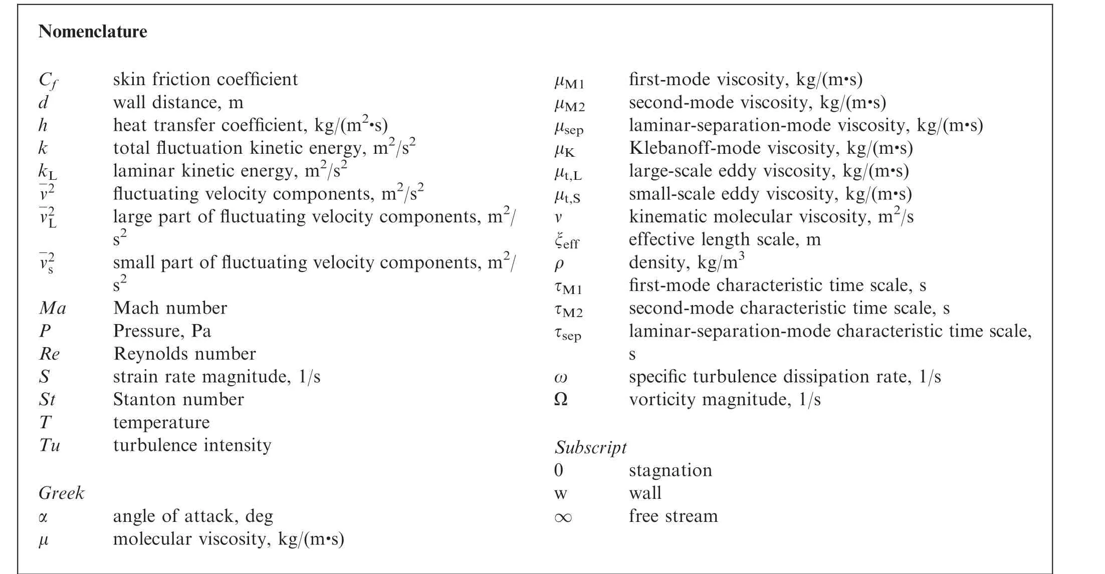
Nomenclature Cf skin friction coefficient d wall distance， m h heat transfer coefficient， kg/(m2·s)k total fluctuation kinetic energy， m2/s2 kL laminar kinetic energy， m2/s2 v－2 fluctuating velocity components， m2/s2 v－2L large part of fluctuating velocity components， m2/s2 v－2s small part of fluctuating velocity components，m2/s2 Ma Mach number P Pressure， Pa Re Reynolds number S strain rate magnitude， 1/s St Stanton number T temperature Tu turbulence intensity Greek α angle of attack， deg μ molecular viscosity， kg/(m·s)μM1 first-mode viscosity， kg/(m·s)μM2 second-mode viscosity， kg/(m·s)μsep laminar-separation-mode viscosity， kg/(m·s)μK Klebanoff-mode viscosity， kg/(m·s)μt，L large-scale eddy viscosity， kg/(m·s)μt，S small-scale eddy viscosity， kg/(m·s)ν kinematic molecular viscosity， m2/s ξeff effective length scale， m ρ density， kg/m3 τM1 first-mode characteristic time scale， s τM2 second-mode characteristic time scale， s τsep laminar-separation-mode characteristic time scale，s ω specific turbulence dissipation rate， 1/s Ω vorticity magnitude， 1/s Subscript 0 stagnation w wall∞ free stream

In recent decades， a variety of approaches have been proposed for predicting transition in Computational Fluid Dynamics (CFD) simulations. These approaches include empirical correlations， emethods， Reynolds-Averaged Navier–Stokes (RANS) models， Large Eddy Simulations(LES)and Direct Numerical Simulations(DNS).Empirical correlations and emethods have been used successfully in engineering applications， although their lack of university and the involvement of non-local variables or operations limit their application in today’s parallel CFD codes.LES and DNS have made great contributions to revealing physical mechanisms in transition processes. For example， Smith and Ventikosinvestigated the transition behavior over an airfoil using LES and DNS， and Lu et al.studied the transitionshielding effects in compressible boundary layers. However，because of the very high calculational expense of these approaches，LES and DNS are rarely used in engineering practice. Therefore， taking into consideration the balance between computational accuracy and expense，RANS-based transitionsensitive models have attracted much interest for engineering transition prediction.

The transition-sensitive models that have been developed in the RANS framework can be divided into two groups. In the first group， empirical correlations or emethods are coupled with fully turbulence models. This type of approach is easy to implement but still uses nonlocal variables or operations.The models in the second group modify existing equations and/or add additional equations in the framework of a turbulence model. These models can generally be divided into two groups: correlation-basedand physics-based. In the correlation-based models， experimental transition criteria are applied to the transport equations in a local fashion. A representative model is the well-known γ-Remodel. In this model， the effects of different factors in experimental correlations are taken into consideration by a transport scalar ～Re，namely the local transition onset momentum thickness Reynolds number. The laminar-turbulent transition is triggered by the intermittency factor γ， which is obtained from another transport equation.Various validations have proved this model’s ability to predict transitions caused by the T-S waves，freestream turbulence intensity and Laminar Separation Bubble(LSB).Further developed by different groups，the γ-Remodel has been extended to apply to crossflow instabilityand roughness effects.

Without the need to apply transition correlations， physicsbased models have significant advantages because the physical mechanisms are introduced directly. Considering instability modes in the pretransitional region， Warren et al.proposed the use of an effective eddy viscosity μ， which is a weighted sum of a turbulent part μand a nonturbulent part μ.μis a function of characteristic timescales associated with different instability modes. As a successor to the concept of effective viscosity， Wang and Fudeveloped a k-ω-γ model appropriate for transitional flows within supersonic/hypersonic flows. Here， k represents the total fluctuation kinetic energy and γ is used to weight μand μin μ.Further developed by Wang et al.， Xu and Fu， Zhou et al.， Yang and Xiao， the k-ω-γ model has been extended for bypass，crossflow-induced and distributed-roughness-induced transitions.

Another popular physics-based transition modeling approach is the Laminar Kinetic Energy (LKE) framework.The core concept of this method is the modeling of laminar kinetic energy k. Mayle and Schulzfirst proposed a ktransport equation to describe high-amplitude pretransitional streamwise velocity fluctuations. Walters and Leylekdeveloped a ktransport equation using the traditional strainbased production mechanism and coupled it with the k-ε model.Walters and Cokljatinherited this idea and proposed the k-k-ω model. In the k-k-ε and k-k-ω modes， the transition is described by the transfer of energy from turbulent kinetic energy kto k， which is represented by model terms with opposite signs in kand kequations. Although the kk-ε and k-k-ω modes are very empirical due to the use of numerous transition threshold functions， they are commonly classified as physics-based models because they describe the production of laminar fluctuations and the transfer of energy from laminar to turbulent fluctuations. Recently， Lopez and Watersimproved the k-k-ω model by using a new transport scalar v.This new model is called the k-v-ω model，where k represents the total fluctuation kinetic energy and vdescribes the fluctuating velocity components normal to the streamwise direction. Because the LKE framework is built completely on local variables and is easy to implement in CFD codes， a wide range of models have been developed further in this framework. For example， Medina and Earlyimproved the k-k-ω model for predicting transitions induced by backward-facing steps. Li et al.proposed an improved k-v-ω model for aerodynamic prediction of iced airfoils.These investigations have demonstrated the flexibility of the LKE framework in transition prediction. However， the LKE models described above are generally used for simple configurations and low-speed flows.Besides，only T-S waves and Klebanoff modes are considered， which makes the k-k-ω and k-v-ω models inapplicable to high-speed transitional flows，crossflow instability and separation-induced transition.

This paper focuses on developing a new physics-based model for transition predictions in a wide speed range. Based on the LKE concept， kis used to describe pretransitional streamwise velocity fluctuations. The different transition mechanisms， natural， bypass and separation-induced transition，are considered in the production of kwith the aid of stability theories. vis chosen to describe the fluctuating velocity components normal to the streamwise direction.The transition process is triggered automatically with the development of prestransitional velocity fluctuations. After the transition process has finished， the model reverts to the Wilcox 2006 k-ω turbulence model.

In Section 2.1， the new model concept is presented. Subsequently， the detailed model formulation is introduced in three parts: the transport equation for laminar kinetic energy (Section 2.2)， the transport equation for fluctuating velocity components (Section 2.3)， and the full model formulation(Section 2.4). The mode validation is presented in Section 3.Finally， Section 4 presents the conclusions.

2. Model formulation

2.1. New model concept

The key feature of the present model is the modeling of pretransitional velocity fluctuations. Different modeling approaches of khave been proposed in recent years.The production mechanism of kin Mayle’s modelderives from the pressure diffusion term in the kinetic energy budget. Walters and Leylekpointed out that the growth of kis due to the Reynolds stresses correlated with pretransitional velocity fluctuations and the mean shear.Thus，in the k-k-ε and k-k-ω model， the traditional strain-based production mechanism is applied in the kequation.Besides，in the kproduction term，the natural transition is considered by assuming that the selfsustained instability mechanism can be modeled through a timescale proportional to the vorticity magnitude Ω. Moreover， in the experimental investigation of backward-facing steps， Wang and Gaterfound that the transition Reynolds number is associated with the N-factors calculated from Linear Stability Theory (LST). These features suggest the production of kcan be modeled using timescales based on wave amplification/stability approaches.

Another transport scalar vhas a dual meaning.In the freestream， laminar and pretransitional regions， vrepresents the energy of fluctuating velocity components normal to the streamwise direction.When the transition process is complete，such as in fully turbulent regions， vcorresponds to the fully turbulent fluctuation energy. Following the concept of Refs.， transition processes correlate with the pressurestrain terms in the Reynolds stress equations. In the laminar region， these terms are suppressed. In the pretransitional region，they are triggered，which leads to an increase in kinetic energy in the fluctuating velocity components normal to the streamwise direction(v)and results in the activation of turbulent production.The concept of the variable vhas been widely adopted in the literature， and the relationship between vand boundary layer transition has also been noticed. vwas originally employed in the k-ε model to represent velocity fluctuations normal to mean flow streamlines. This variable has also been used to reflect pressure-strain term effects in linear eddy viscosity turbulence models. Besides， both experimentaland analyticalinvestigations have shown that the growth of kis associated with the normal fluctuations of the freestream turbulence， which is represented by v. Other studieshave also demonstrated that the wall-normal turbulence causes the Klebanoff-mode production and the initiation of the transition process is correlated with a rapid rise in wall-normal fluctuation kinetic energy. These features suggest the feasibility of a transition model based on modeling the pretransitional velocity fluctuations.

2.2. Transport equation for laminar kinetic energy

As discussed above， the laminar kinetic energy krepresents the streamwise velocity fluctuations in the pretransirional region. Similar to the work of Papp and Dashand Xu et al.， the ktransport equation in this paper is expressed as follows:

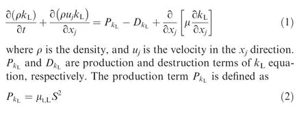
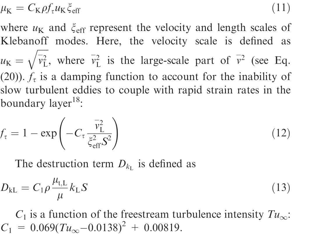
where μis the large-scale eddy viscosity.In the present work，μis taken to consist of the first-mode viscosity μ， the second-mode viscosity μ， the laminar-separation-mode viscosity μand the Klebanoff-mode viscosity μ.

where E= 0.5|U|represents the kinetic energy of the mean flow， and U is the local velocity magnitude.

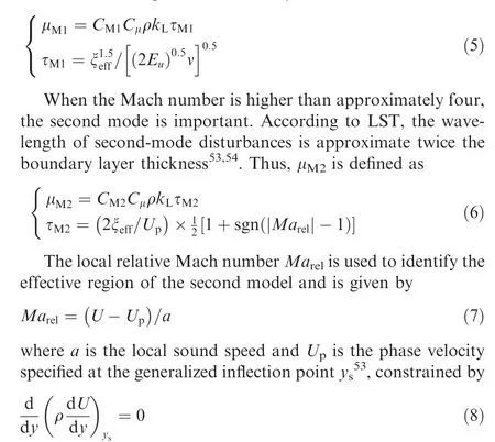
From LST and experimental investigations， the first mode(i.e.，T-S waves in low-speed flows)dominates the natural transition in low Mach number flows. From the experimental correlation of the frequency of the first mode disturbances with the maximum amplification rate， μcan be modeled as

For the laminar-separation-induced transition， according to the stability analyses of the Kelvin-Helmholtz instability in the separated shear layers conducted by Monkewitz and Huerre， the laminar-separation-mode viscosity μcan be modeled as

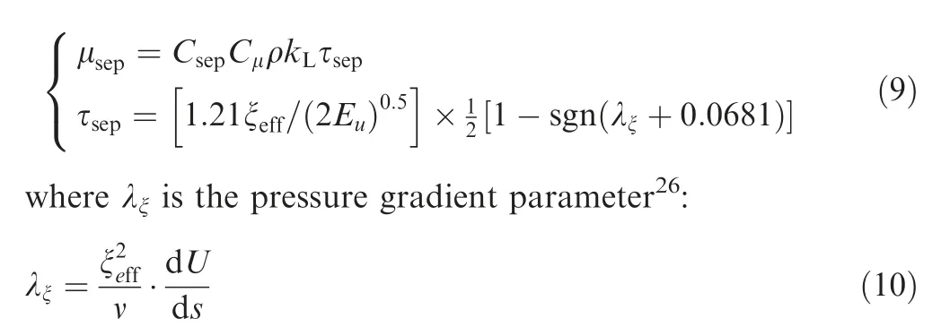
where dU/ds is the acceleration along the streamwise direction.The critical value of λin Eq.(9)is set as－0.0681 according to the laminar separation analysis of Menter et al.

When the freestream has a high turbulence level， bypass transition becomes the main transition mechanism. Bypass transition is characterized by the birth of streak-shaped velocity fluctuations， which are called Klebanoff modes. According to previous studies， the growth of Klebanoff modes is dominated by the wall-normal freestream turbulence. Following this concept， the Klebanoff-mode viscosity is defined as

2.3. Transport equation for fluctuating velocity components

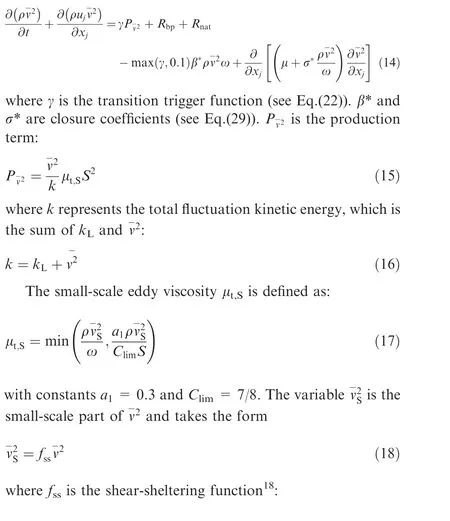
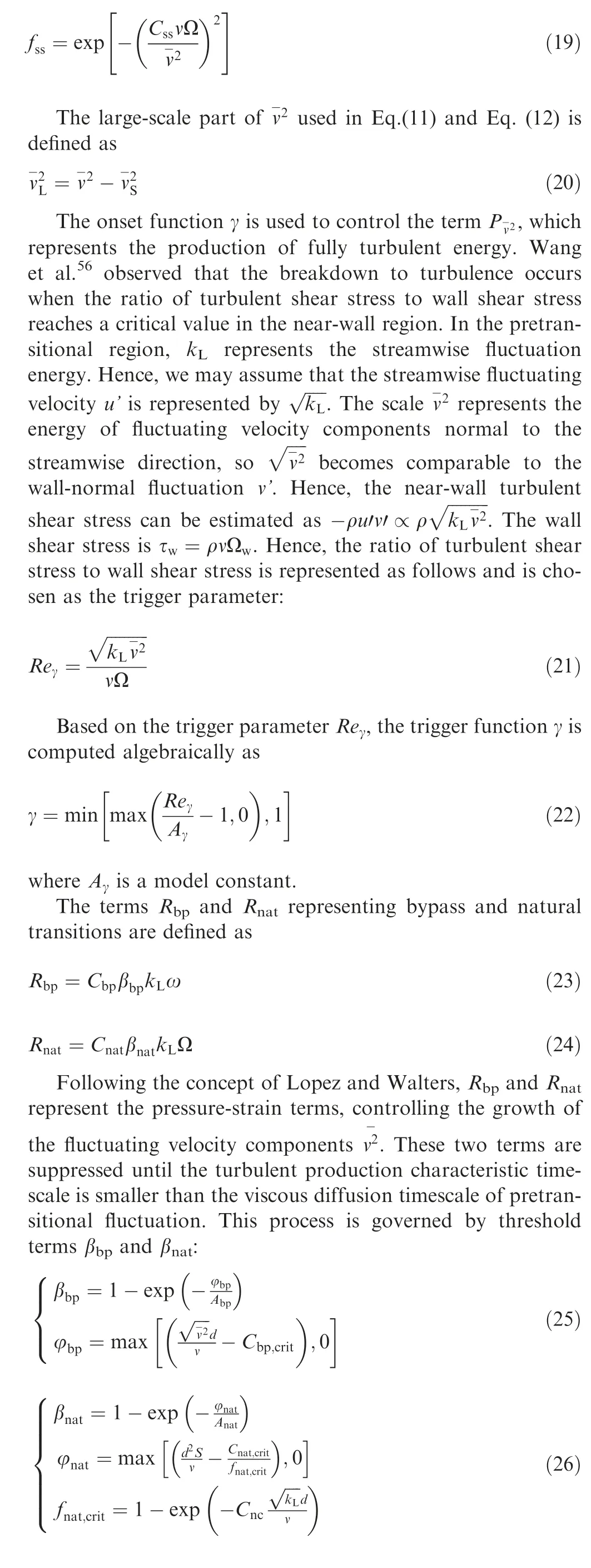
The transport equation of vused in this paper is similar to that proposed by Lopez and Walters and is expressed as follows:

2.4. Full formulations of the transition model

The full transition model is a three-equation model.Transport equations are solved for the laminar kinetic energy，the fluctuating velocity components，and the specific turbulence dissipation rate:

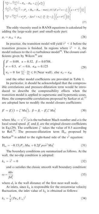
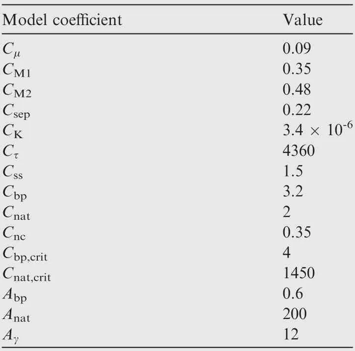
Table 1 Summary of model coefficients.

where Uis the freestream velocity magnitude.

Besides， the total fluctuation energy is commonly obtained using the freestream turbulence intensity Tubased on the assumption of isotropy:

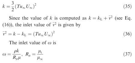
The prediction procedure for boundary layer transition using the present physics-based transition model is as follows.The inlet values of kand vare calculated using the freestream turbulence intensity Tu. Based on LST， the largescale eddy viscosity μis calculated considering different transition mechanisms and contributes to the production of k. Once the characteristic timescale for turbulence production is smaller than the viscous diffusion timescale of the pretransitional fluctuations， the model terms Rand Rare activated， corresponding to an increase in v. With the development of kand v， the onset function γ will be triggered when the onset parameter Rereaches a critical value. Then，the production term of vis activated， leading to the growth of the fully turbulent energy. When the transition process is finished， the present model reduces to the k-ω turbulence model.

3. Model validation

The new physics-based model is validated by several test cases，including flat plates， airfoils and straight cones. The flat plate cases in Section 3.1 are used to calibrate the model coefficients.After the calibration，the model is employed for the remaining cases.

The numerical simulations in this paper are based on an inhouse finite volume CFD solver MI-CFD， which is developed by the authors. The spatial discretization for the inviscid fluxes of the Navier-Stokes equations use the Monotone Upstream-centered Scheme for Conservation Laws (MUSCL)and Roe’s flux difference splitting method. The implicit Low-Upper Symmetric Gauss-Seidel (LUSGS) method is applied for time marching.

3.1. Full formulations of transition model

3.1.1. Zero-pressure-gradient flat plate

The model is first calibrated by Zero-Pressure-Gradient(ZPG)flat plate cases， including the T3A and T3B series experimentsand the Schubauer and Klebanoff (S&K) case. The inlet conditions are presented in Table 2. Constant inlet air properties are adopted as follows: ρ=1.2 kg/mand μ=1.8 × 10kg/(m·s).

A grid convergence study for the S&K flat plate test case is conducted to preserve the high grid resolution inside the boundary layer. Four grids (marked by G1-G4) were generated to analyze the grid convergence， which provides a comparison for the non-dimensional wall distances (y) ranging from 0.5 to 3.0. The computational grid is shown in Fig. 1.The upstream region of the flat plate has 31 nodes in the streamwise direction for all grids. The detailed information for different grids is listed in Table 3，where dmeans the wall distance of the first near-wall node， Nand Nrepresent the node numbers in the streamwise direction and normal direction， respectively.

Fig.2 shows the predicted skin friction coefficients Cdistributions for the four grids， where Re= ρUx/μis the local Reynolds number based on the local streamwise position x and freestream parameters. It is obvious that Cin the laminar region is in good accordance with each other for the four grids. The transition onsets almost locate the same position when yis below 1.0.In the turbulent region，there is only a modest increase for Cas the ydecreases from 3.0 to 0.5，and the amplification decreases as well. Since the distinction between the results from grids G3 and G4 is negligible， it can be concluded that thegrid convergence is well established.The following computations are based on G3 resolution level.

Fig.3 shows the predicted skin friction coefficients Cdistributions.The experimental measurements and numerical results from two popular transition models， namely γ-Reand k-kω， are also shown for comparison. For the T3B case in Fig. 3(a)， the freestream turbulence intensity is relatively high， leading to an early transition. The present model successfully captures the transition onset and the evolution of C.However，the peak value from computation is marginally lower than the experimental measurement. The γ-Remodel accurately cap-tures the maximum of C， while the laminar value is overpredicted. The k-k-ω model computes the accurate laminar value， but the predicted transition is marginally delayed.Moreover，the result of the k-k-ω model exhibits an obvious overshoot phenomenon during the transition process. For the T3A case in Fig.3(b)，the Tuis relatively moderate.The present model and the γ-Remodel both show excellent results，while the k-k-ω model predicts a delayed transition onset and a short transition region. For the T3A-case in Fig. 3(c)，the freestream turbulence level is lower than 1%.The predicted transition onset from the present model is marginally overestimated. The γ-Remodel accurately predicts the transition onset， while the transition behavior reproduced by k-k-ω is much in advance.For the S&K case in Fig.3(d)，the freestream turbulence level is relatively low， with the dominant transition mechanism being natural transition. From this comparison of the results， we can see that the transition onset obtained from the present model is marginally underestimated compared with that from γ-Remodel and the measured data.For the k-k-ω model， the transition onset in its results is too early. Overall，the present model predicts the transition behavior of ZPG flat plate cases with good precision. The γ-Remodel also gives convincing results， but the k-k-ω model always predicts early transition at low turbulence levels.

Table 2 Flow inlet conditions for ZPG flat plate cases.

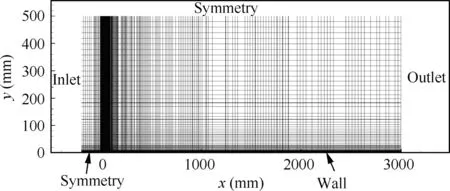
Fig. 1 Computational mesh of ZPG flat plate test cases.

Fig.4 and Fig.5 present the streamwise velocity u and total fluctuation kinetic energy k profiles for T3A case.The profiles are obtained at streamwise locations Re= 10(laminar region)，2.25×10(transitional region)and 5×10(turbulent region). u and k are nondimensionalized by Uand U，respectively， where Uis the freestream velocity. δ denotes the boundary layer thickness.In the laminar region，the agreement between the calculational result and measured data is excellent. In the transitional region， a slightly underprediction can be seen near y/δ ≈0.2.In the turbulent region，the predicted result shows good consistency with the experimental data， while slight over-prediction can be seen near y/δ ≈0.3. In Fig. 4， the present model can qualitatively predict the total fluctuation kinetic energy at all three streamwise loca-tions. In the laminar and transitional regions， the peak values computed from the present model are farther from the wall compared with the experiment. In the turbulent region， the predicted results show a similar tendency to the measurement，while the peak value is under-predicted. Overall， the present model predicts the streamwise velocity and fluctuation kinetic energy with reasonable accuracy.

Table 3 Detailed information for different grids.

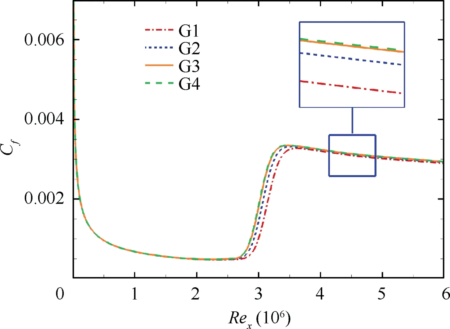
Fig. 2 Grid convergence study for S&K flat plate test case.

3.1.2. Flat plate with laminar separation bubble

T3L test cases，with 10 mm leading-edge diameter，are simulated to assess the new model’s capability for separationinduced transition.The computational setup is consistent with the numerical investigation of Wang et al.The inlet velocity is 5 m/s，the freestream Reynolds number is 3.29×10/m and the freestream turbulent intensities vary from 0.63%to 5.34%.The computational mesh has 351 and 151 nodes in streamwise and wall-normal directions， respectively. The normal distance of the first cell to the wall is specified in order to maintain y＜1. A close-up of the mesh at the leading edge region is shown in Fig. 6.

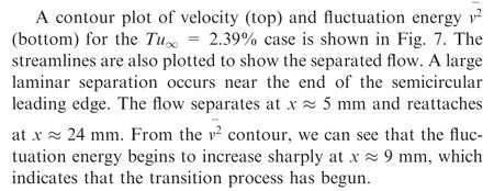
Fig. 8 compares the computed Cwith the experimental results.The separation point is the location where C=0 first appears. Downstream of the separation point， a recirculation zone appears and leads to a negative value of C. At the reattachment point， Cincreases from negative values to zero.Note that in the experimental data，when the value of Cis negative，Cis set to zero.The comparison shows that the present model accurately captures the separation and reattachment positions at different freestream turbulence levels. Moreover，the model successfully reflects the influence of freestream turbulence intensity. As Tuincreases， the computed reattachment position gradually moves forward.

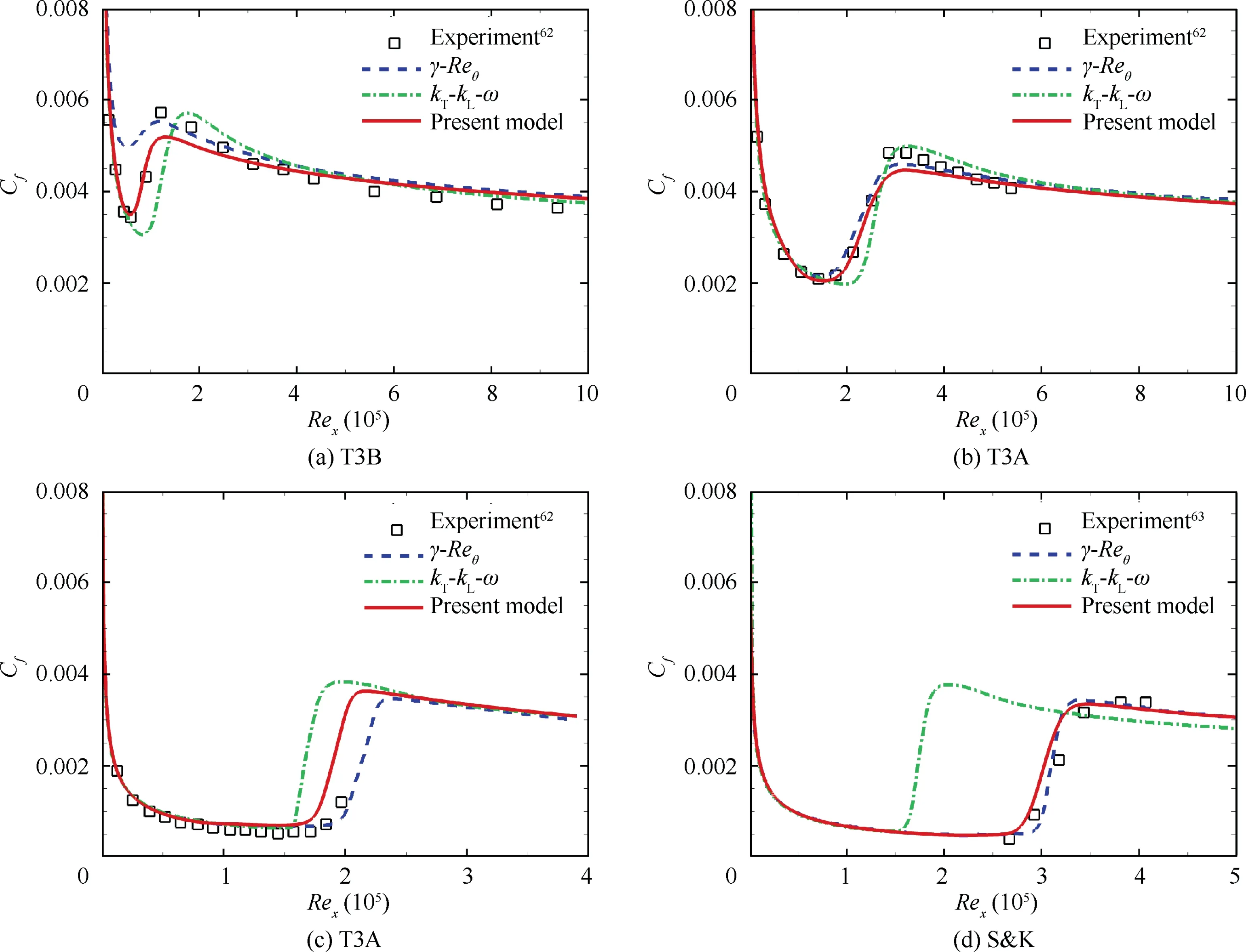
Fig. 3 Skin friction coefficient for ZPG flat plate cases.

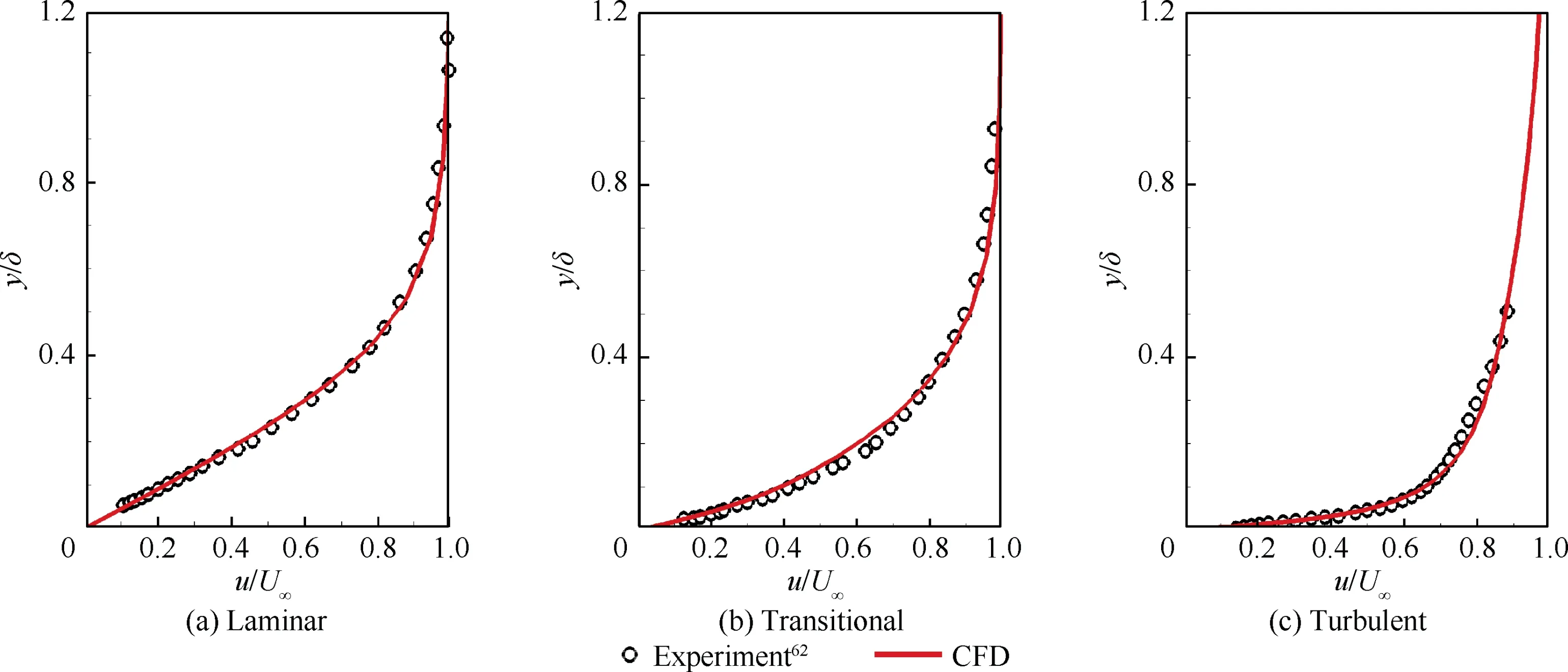
Fig. 4 Velocity profiles for T3A case.

Fig. 9 presents the velocity profiles across the separation bubble for the Tu= 2.39% case. The vertical axis variable‘‘d”means the normal distance from the wall.From the comparison，it is obvious that the model accurately predicts velocity distributions.In the separation bubble，because of the recirculation zone， the near-wall velocity has a negative value.At x =6 mm，the peak value of the negative velocity is small，and its location is near the wall. As the separation bubble develops， the peak value of the negative velocity increases，and the velocity profile moves away from the wall.When x is greater than 15 mm， as the flow enters the pressure recovery zone and moves towards reattachment， the peak value of the negative velocity reduces.Moreover，from the distribution of velocity profiles，we can see that an inflection point exists and provides a source of instability.

3.1.3. Hypersonic flat plate

To calibrate and verify the model for high-speed flows， a hypersonic flat plate is simulated. The freestream conditions are chosen from the experiment of Mee， as listed in Table 4;Tu=0.4%，T=300 K，and μ/μ=0.001 are applied for all cases.The computed mesh has 501 and 151 nodes in streamwise and wall-normal directions，respectively，with a maximum y＜1.

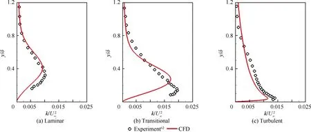
Fig. 5 Total fluctuation kinetic energy profiles for T3A case.

Fig.10 compares the predicted and measured Stanton number St. From the comparison， we can see that the agreement between computation and measurement is excellent. The present model accurately predicts the transition onset and a similar development trend of St compared with the experiment.Simultaneously， as Reincreases， the transition onset moves forward and the transition region shortens， which indicates that the present model can reasonably reflect the Reeffects.

Instability modes are considered in the present model. For further analysis of Reynolds number effects， the profiles of first-mode viscosity μ， second-mode viscosity μand laminar kinetic energy kat x = 300 mm (laminar region) are shown in Fig.11.μand μhave been nondimensionalized by the freestream molecular viscosity μ， and khas been nondimensionalized by U. From the comparison， we can see that the peak values of μis greater than that of μ.Besides， the peak position of μis much closer to the wall than that of μ. These phenomena indicate that the second mode maters the development of knear the wall， which is in accord with LST theory: the second mode dominants the transition when the Mach number is greater than approximately four. Moreover， the values of both μand μincrease as Reincreases， leading to a greater k. Thus， the Reeffects on transition are contained in the development of instability modes in the present transition model.

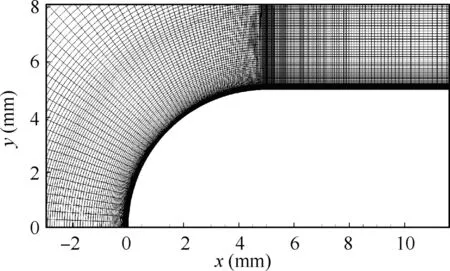
Fig. 6 Mesh close-up at leading edge region of T3L test cases.

Fig. 7 Contours of velocity (top) and fluctuation energy(bottom) for Tu∞= 2.39% case.

3.2. Airfoil test cases

Flow over airfoils is a typical example for which transition plays an important role. Transition affects skin friction distributions and separation locations on airfoil surfaces. In this section，two airfoil test cases are presented to asses the model’s ability to capture transition behavior on airfoils.

3.2.1. Aerospatiale-A airfoil

The first airfoil test case is the Aerospatiale-A airfoil.The freestream conditions used for numerical simulations are chosen from the experiment in the ONERA F1 wind tunnel， as follows: Re=2.1× 10(based on the chord length C=1 m)，Ma=0.15，α=13.1°，Tu=0.2%and μ/μ=10.0.The computational mesh are shown in Fig.12.The wall-normal cell number is 201，with a maximum y＜1.0;the chord-wise cell number is 301 on each wing side.

Fig. 8 Skin friction coefficient distributions for T3L cases.

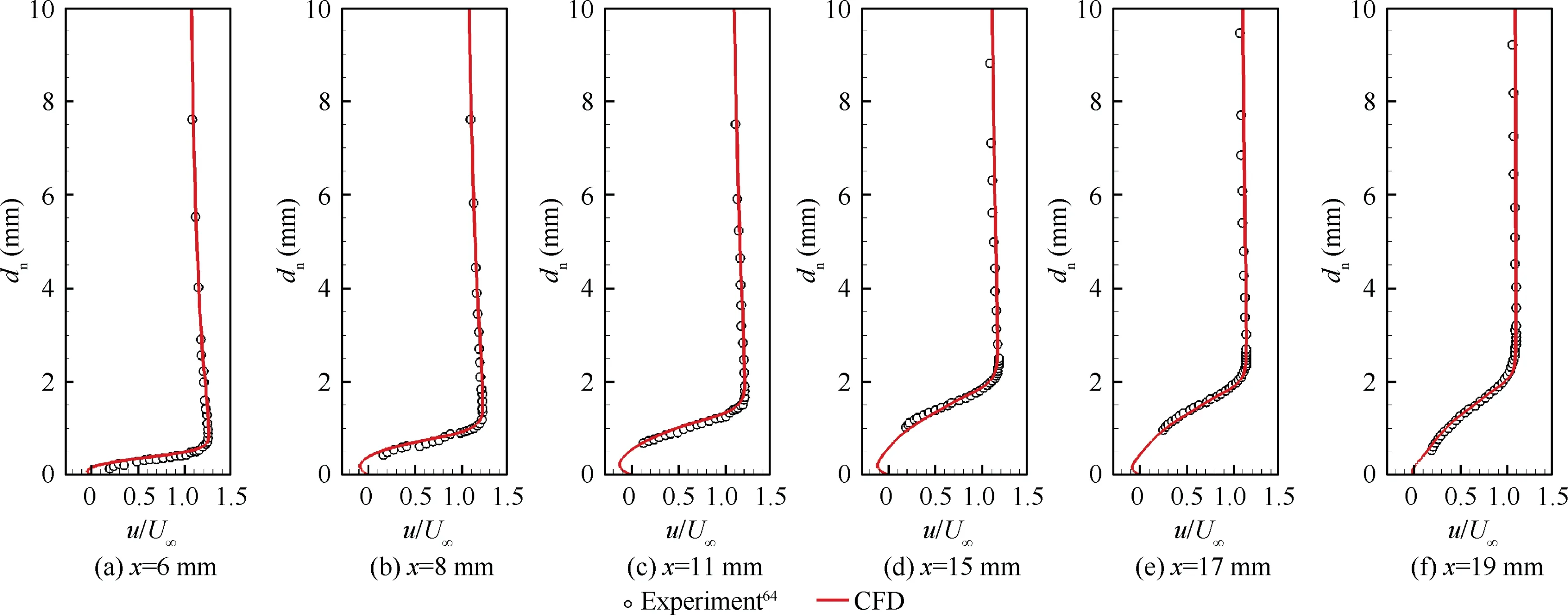
Fig. 9 Velocity profiles across separation bubble for Tu∞= 2.39% case.

Fig. 13 shows the computed and measured Cdistributions on the suction side. The present model accurately reproduces the transitional flow around the airfoil. From the computed result， we can see that the flow separates at approximately 8.8% of chord and reattaches at approximately 11.5% of the chord. This small separation bubble induces a separationinduced transition， which causes a sharp increase in C.Fig. 14 illustrates the details of the LSB and the contours of the transition onset function γ. We can see that γ grows to unity quickly after the separation point. This phenomenon reveals the reasonableness of the transition onset function and demonstrates the model’s capability of capturing the separation behavior on airfoils.

Table 4 Freestream conditions for hypersonic flat plat cases.

3.2.2. NLR-7301 airfoil

The NLR-7301 airfoil is a representative thick supercritical airfoil and has been used in many experimental investigations in the transonic range. Previous investigationshave shown that with changes in Maand α， the transition on the NLR-7301 airfoil occurs in different paths， including natural transition and separation-induced transition. In this section， transitional flows at Re= 2.2 × 10(based on a chord length C=1 m)with Mach number varying from 0.3 to 0.8 are simulated， with Tu= 0.2% and μ/μ= 10.0. The corrected α used for simulation is the same as that in Ref.. The computational mesh is shown in Fig. 15， and the grid resolution is similar to that for the Aerospatiale-A airfoil.

The predicted and measured transition locations are shown in Fig. 16. On the pressure side， the transition locations are slightly underestimated. At the suction side， the transition onsets are predicted well， except for the Ma= 0.724 and 0.748 case. From the comparison， we can conclude that the variations of transition onsets with Maare predicted with reasonable precision on the NLR-7301 airfoil.

Fig. 10 Stanton number distributions for hypersonic plate cases.

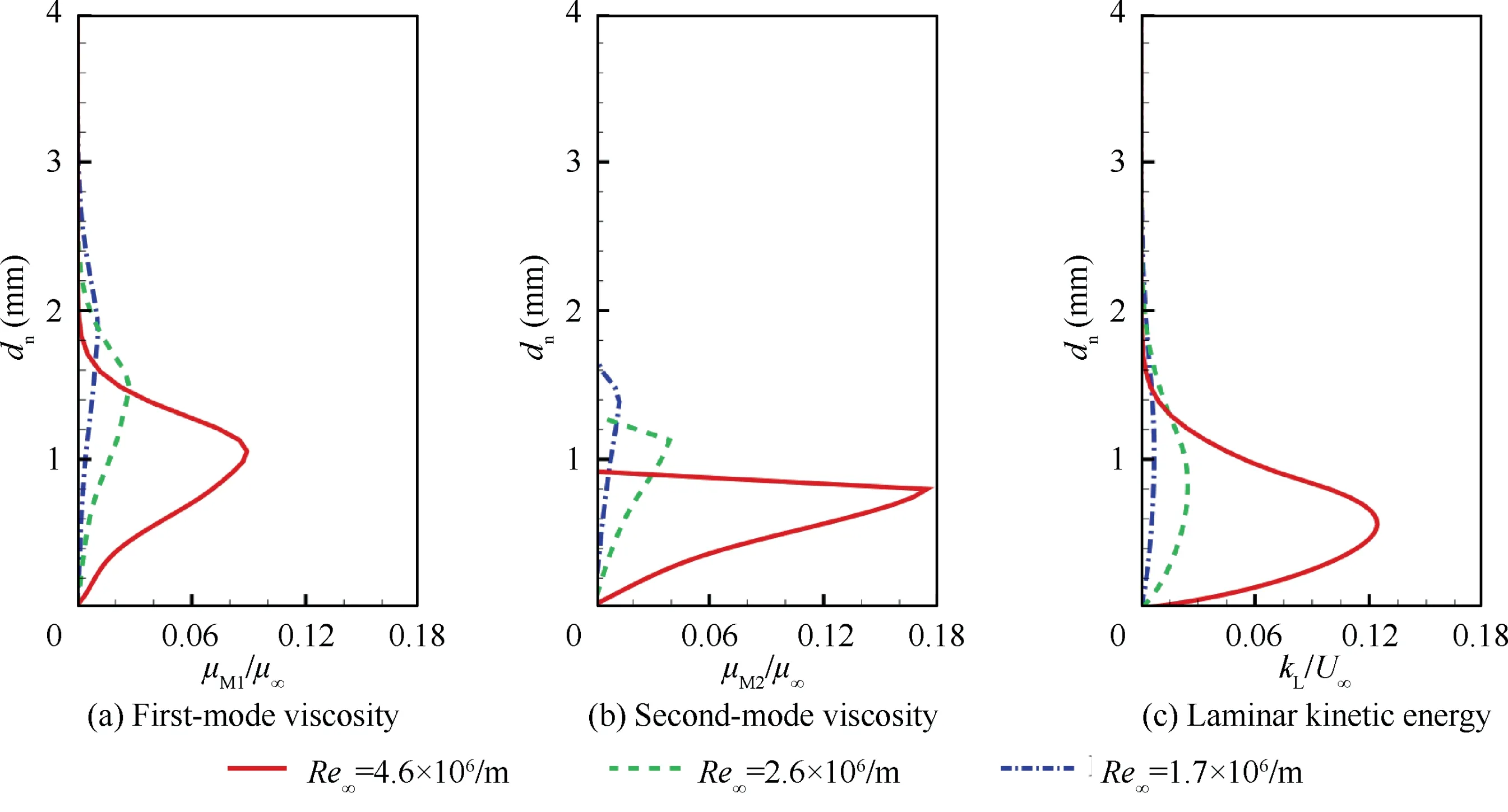
Fig. 11 Profiles of flow variables at x = 300 mm (laminar region).

From Fig. 16， we can see that the transitions on the pressure side all occur in the region of 0.55C to 0.60C and are not sensitive to changes in Ma. On the suction side， transition onsets are in the region of 0.12C to 0.18C when Mais less than 0.7.At Ma=0.724，the transition onset moves significantly backward.As Macontinues to increase，the transition occurs in the region behind 0.6C. For further analysis of the reason for this behavior， Fig. 17 presents the predicted and measured pressure coefficient Cdistributions at four Mach numbers (0.6， 0.7， 0.724 and 0.774). For all four Mach numbers， the agreement is excellent， and a favorable pressure gradient is maintained on the suction side until the mid region of the airfoil. At the 0.5C position， a strong adverse pressure gradient occurs， which leads to transition occurring near 0.55C and remaining insensitive to variations in Ma. As for the suction side， a strong adverse pressure gradient occurs near the leading edge(see Fig.17(a)to 17(c))and leads to early transition in the region near 0.2C，except for the Ma=0.774 case. When the Mach number increases to 0.774， a flat roof pressure distribution persists on the suction side until the position near 0.6C， and the transition onset moves backward significantly.

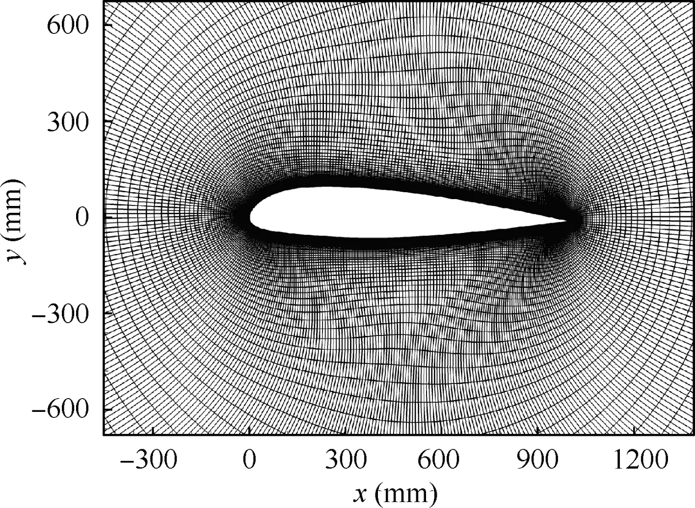
Fig. 12 Computational mesh around the Aerospatiale-A airfoil.

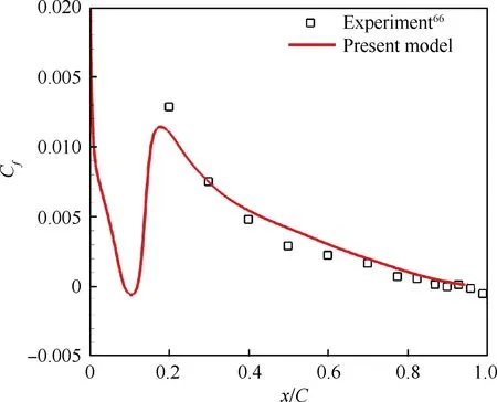
Fig. 13 Cf distributions on suction side of Aerospatiale-A airfoil.

3.3. Adiabatic straight cone at Ma∞=3.5

To further validate the performance of the model for highspeed transitional flow， 5° half-angle adiabatic straight cone test cases are simulated. This test case is chosen from the experiment of Chen et al.. The cone has a length of 381 mm and a nose bluntness of 0.025 mm. The freestream conditions are taken as follows: Ma= 3.5， α = 0°， Tu= 0.1% and μ/μ= 0.001. Other freestream conditions are provided in Table 5， in which Tand Pare the total temperature and total pressure， respectively. The half model grid employed has a total of more than 4 × 10grid cells; there are 201 wall-normal grid nodes， with a maximum y＜1. It is noted that the freestream turbulence intensity Tuis computed using the following equation， as suggested by Wang et al.:

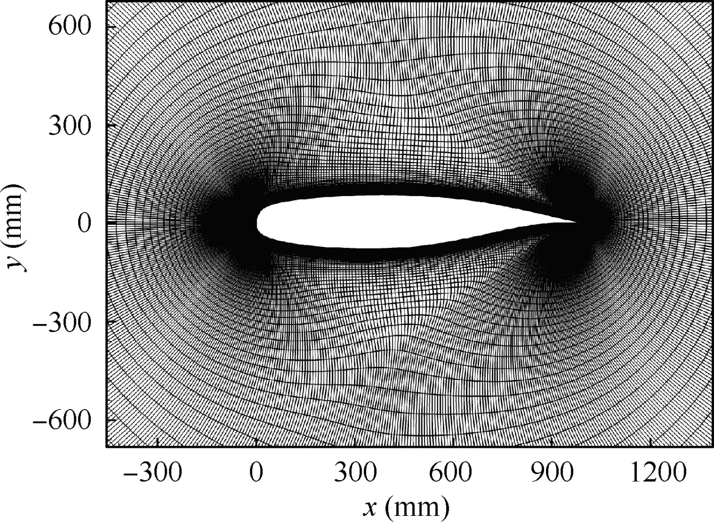
Fig. 15 Computational mesh around NLR-7301 airfoil.

where PL is the measured pressure fluctuation， which is set to 0.4% according to the experiment. γis the specific heat ratio.

Fig. 18 compares the computed skin friction coefficient Cwith the measured temperature recovery factor r. From the comparison， we can see that although there is slight underprediction or over-prediction of the transition onset， the present model reproduces the transition behaviors under different freestream conditions with reasonable accuracy. In particular，the calculated transition length exhibits good consistency with the experimental measurements.Moreover，the predicted transition occurs early and the transition length decreases with increasing Re， which shows the model’s ability on capturing the Reeffects in high-speed transitional flows.

Fig.19 presents the distributions of flow variables along the wall-normal direction at x = 60 mm (laminar region). As shown in Fig. 19(a)， the strain rate magnitude S in the nearwall region increases with increasing Re.Therefore，the peak value of the effective length scale ξgradually moves closer to the wall because it is in proportion to S，as shown in Fig.19(b).The greater ξleads to a greater first-mode viscosity μwith increasing Reynolds numbers， which causes early transition.Since the freestream Mach number is less than four， the second-mode viscosity μis zero， and the second mode does not influence the transition process.

3.4. Straight cone at Ma∞=6.0

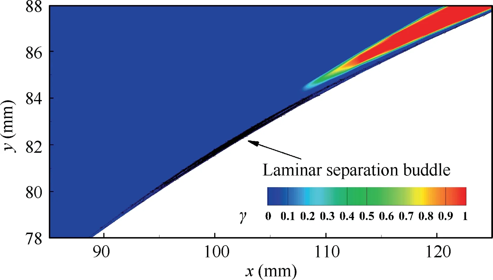
Fig. 14 Contours of transition onset function γ around laminar separation bubble on Aerospatiale-A airfoil.

A hypersonic straight cone is simulated in this section. This test case is the same as the experiment of Horvath et al.The 5° half-angle isothermal cone has a length of 635 mm and a nose bluntness of 0.00254 mm. The freestream conditions are taken as follows: Ma= 6.0 ， α = 0°， T/T= 0.59， Tu= 0.4% and μ/μ= 0.001. The freestream turbulence intensity Tuis computed from Eq. (38) based on the measured PL = 3.4%. Other flow conditions are provided in Table 6. The half model grid employed has a total of more than 5×10grid cells;there are 221 wall-normal cells，with a maximum y＜1.

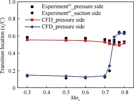
Fig. 16 Transition location xt/C as a function of Mach number for NLR-7301 airfoil.

The predicted and measured dimensionless wall heat flux h/hdistributions for four cases are shown in Fig. 20. Here，h = q/(H－H)， where q is the heat transfer rate， and Hand Hare the adiabatic and isothermal wall enthalpies，respectively.his the reference value obtained from the Fay-Riddell theory. In Fig. 20(a)， the transition onset is predicted well， while the transition length is a little under-predicted. In Fig. 20(b) and Fig. 20(c)， the predicted results exhibit good consistency with the experiment. As for the lowest Recase in Fig. 20(d)， the transition onset is marginally overpredicted. Moreover， the present model can successfully predict the same trend with changes in Reas the experimental results.

Fig.21 presents the distributions of flow variables along the wall-normal direction at x = 150 mm (laminar region). The distributions and development trends of S and ξin Fig. 21(a) and 21(b) are similar to these in the Ma = 3.5 test cases(see Fig. 19(a) and 19(b)). However， obvious differences can be seen in the distributions of μand μ. Because Mais now up to 6.0， the boundary layer edge Mach number is greater than 4，and the second mode becomes the major disturbance source. The second mode leads to a small magnitude of μand a large magnitude of μ，as shown in Fig.21(c) and 21(d)， and the peak value of μis approximately three times greater than that of μ.Moreover，the peak position of μis much closer to the wall than that of μ. This is consistent with the findings in Section 3.1.3 (see Fig. 11).

4. Conclusions

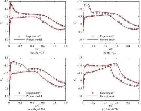
Fig. 17 Pressure distributions under different Mach numbers for NLR-7301 airfoil.

Table 5 Freestream conditions for Ma∞=3.5 straight cone.

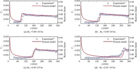
Fig. 18 Computed skin friction coefficient and experimental recovery factor distributions for Ma∞= 3.5 straight cone.

Fig. 19 Distributions of flow variables at x = 60 mm for Ma∞= 3.5 straight cone.

Table 6 Freestream conditions for Ma∞=6.0 straight cone.

The new model has been calibrated and validated primarily by application to flat plate flows， including zero-pressuregradient cases， laminar separation bubble cases and highspeed cases.It has then been validated by application to airfoil test cases and high-speed straight cones. For the subsonic flat plate and airfoil cases， the prediction results show generally good agreement with experimental data， which applies both to global quantities such as transition onset and separation point，as well as for local skin friction and surface pressure distributions. For the supersonic and hypersonic cases， the present model results in a proper response to the freestream Reynolds number， although the model is unable to capture the overshoot phenomenon of aeroheating. Further investigation is needed to improve the model’s performance in reproducing the overshoot phenomena in transition processes.

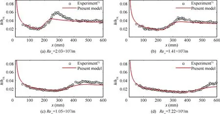
Fig. 20 h/hFR distributions for Ma∞= 6.0 straight cone.

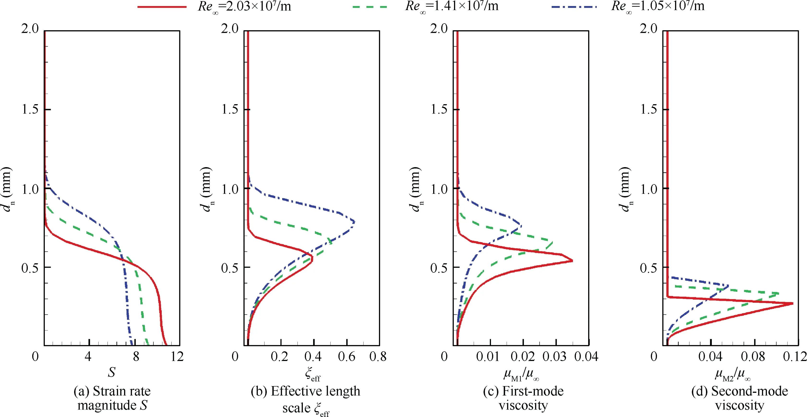
Fig. 21 Comparisons of flow variables at x = 150 mm for three cases (in laminar region).

The present model can serve as a basis for the extension of additional transition mechanisms， such as rotation and curvature effects， roughness-induced transition， and crossflowinduced transition. However， different mechanisms are taken into consideration by linearly adding eddy viscosities to the large-scale eddy viscosity， and the nonlinear interaction of these mechanisms has been not considered in the current work.In the next step， the interaction between different instability modes will be carried out. Further work also includes validations on three-dimensional and complex configurations.

The authors declare that they have no known competing financial interests or personal relationships that could have appeared to influence the work reported in this paper.

Acknowledgments

This work was supported by grants from the National Natural Science Foundation of China (No. 11721202) and the Academic Excellence Foundation of Beihang University for PhD Students， China.