Bayesian uncertainty analysis of SA turbulence model for supersonic jet interaction simulations

Jinping LI, Shusheng CHEN, Fngjie CAI, Sheng WANG, Cho YAN,*

a School of Aeronautic Science and Engineering, Beihang University, Beijing 100083, China

b School of Aeronautics, Northwestern Polytechnical University, Xi’an 710072, China

c AVIC The First Aircraft Institute, Xi’an 710089, China

d China Academy of Launch Vehicle Technology, Beijing 100076, China

KEYWORDS Bayesian calibration;MAP estimation;SA turbulence model;Supersonic jet interaction;Uncertainty quantification

Abstract The Reynolds Averaged Navier-Stokes(RANS)models are still the workhorse in current engineering applications due to its high efficiency and robustness.However,the closure coefficients of RANS turbulence models are determined by model builders according to some simple fundamental flows,and the suggested values may not be applicable to complex flows,especially supersonic jet interaction flow. In this work, the Bayesian method is employed to recalibrate the closure coefficients of Spalart-Allmaras (SA) turbulence model to improve its performance in supersonic jet interaction problem and quantify the uncertainty of wall pressure and separation length. The embedded model error approach is applied to the Bayesian uncertainty analysis. Firstly, the total Sobol index is calculated by non-intrusive polynomial chaos method to represent the sensitivity of wall pressure and separation length to model parameters. Then, the pressure data and the separation length are respectively served as calibration data to get the posterior uncertainty of model parameters and Quantities of Interests (QoIs). The results show that the relative error of the wall pressure predicted by the SA turbulence model can be reduced from 14.99% to 2.95% through effective Bayesian parameter estimation.Besides,the calibration effects of four likelihood functions are systematically evaluated.The posterior uncertainties of wall pressure and separation length estimated by different likelihood functions are significantly discrepant, and the Maximum a Posteriori(MAP) values of parameters inferred by all functions show better performance than the nominal values.Finally,the closure coefficients are also estimated at different jet total pressures.The similar posterior distributions of model parameters are obtained in different cases,and the MAP values of parameters calibrated in one case are also applicable to other cases.

1. Introduction

The supersonic jet interaction flow is induced by a lateral jet injected into the supersonic crossflow, which occurs in many applications, such as the scramjet combustors, missile Reaction Control Systems (RCS), etc. This flow is a complex fluid dynamic phenomenon including shocks, separation zones,shear layers, etc.With the development of computer technology, more and more researchers apply Direct Numerical Simulation (DNS) and Large Eddy Simulation (LES) to simulate the lateral jet interaction to explore the flow mechanism and get more accurate simulation results.However, the unaffordable computational costs and difficulties in generating high-quality grids make it difficult for them to be popularized in engineering applications.In engineering applications such as aerodynamic design and optimization, ones only focus on the mean flow, and the instantaneous flow is insignificant.Therefore, the Reynolds Averaged Navier-Stokes (RANS)models that can efficiently solve the mean flow are still the workhorse in current engineering applications due to their low computational cost and high robustness.Although there are many turbulence models available for simulation, their accuracy is problem-dependent.In addition, there are some closure coefficients(also called model parameters)in each turbulence model,which are calibrated by the model builder with data from fundamental flows.The values of closure coefficients suggested by the model builder are often referred to as ‘‘nominal” ones. There is no evidence that the nominal values perform well in all types of flows, thus it is necessary to adjust the values of the closure coefficients for a specific type of flow to improve the simulation accuracy.

The Spalart-Allmaras (SA) turbulence modelis a single equation model and has been widely used in engineering applications because it is less computationally expensive and more robust than the multi-equation models.However, in many researches on lateral jet interaction,Menter’s k-ω Shear Stress Transport (SST) modelis more widely used because it performs well in predicting flows involving adverse pressure gradients and pressure-induced boundary layer separation. In the work of Erb and Hosder,it is also found that the separation zone predicted by SA turbulence model is smaller than that predicted by SST turbulence model in the shock waveboundary layer interaction problem. Therefore, the predictive potential of SA turbulence model for such interaction problems needs to be further investigated. The aim of this work is to recalibrate the closure coefficients of SA turbulence model to improve its performance in supersonic jet interaction problem and quantify the uncertainty of the Quantities of Interests(QoIs).

In the process of constructing RANS models, some assumptions are introduced into the turbulence models,which leads to the uncertainty of numerical simulations. The uncertainty caused by the closure coefficients is called parametric uncertainty,and it has attracted the interest of many researchers. Godfrey and Clifffirst adopted sensitivity equation to research the flow sensitivity to turbulence model parameters,and proved the accuracy and effectiveness of this method for sensitivity calculation. Subsequently, Turgeon et al.applied this method to the standard k-ε turbulence model with wall function. They obtained the uncertainty bands of QoIs,and analyzed the sensitivity of QoIs to model parameters in each case. Schaefer et al.utilized Non-Intrusive Polynomial Chaos (NIPC) method to propagate the uncertainty of the model parameters of three commonly used turbulence models (SA model, Wilcox (2006) k-ω model, and SST model). They focused on several transonic flows and analyzed the Sobol indices of various flow variables. In the abovementioned works,the uncertainty of the parameters of the turbulence models was only propagated forward to analyze the uncertainty of the QoIs, and the information contained in the experimental data was not fully utilized to infer the optimal values of the model parameters.

In order to quantify and reduce the uncertainty of turbulence model parameters, and to assimilate the experimental data or other high-fidelity data to infer model parameters,Bayesian inference technique is applied in Computational Fluid Dynamics (CFD).Cheung et al.carried out the first application of Bayesian uncertainty quantification method to turbulence models in the incompressible boundary layer.Edeling et al.performed Bayesian estimation of the parameters of the k-ε turbulence model using boundary layer flow data.They are concerned with the estimation of model inadequacy in RANS simulations, and calculated the Highest Posterior-Density (HPD) intervals to represent the uncertainty of the numerical solution. Furthermore, Guillas,Ray,and Zhanget al. also used Bayesian method to conduct similar analyses for different turbulence models and different flow types. More researches on Bayesian uncertainty analysis can be found in the review by Xiao and Cinnella.

In the Bayesian uncertainty analysis of turbulence models,an additive term or multiplicative term is usually applied to represent the model error (i.e. the discrepancy between model and reality). The explicit additive term may break the laws of physics, becomes entangled with the measurement error, and usually does not improve the predictive power of the model.Therefore, it is necessary to deal with the model error internally. The multiplicative form is an improvement that enables the stochastic models to satisfy some physics laws such as the no-slip wall boundary condition.Embedding stochasticity into the model is also a good choice to handle model error internally.In this work,the embedded model error approachis applied to the Bayesian uncertainty analysis of SA turbulence model, and the parameters of SA turbulence model are recalibrated using the data from supersonic jet interaction experiment.The research contents of this paper are as follows.Firstly, sensitivity analysis is carried out to provide reference for the selection of parameters embedded randomness. Then,the wall pressure data and separation length are used to calibrate model parameters respectively to demonstrate the ability of Bayesian method to obtain information from small datasets. Besides, the calibration effects of four likelihood functions are also compared. Finally, the model parameters are calibrated in different cases (different jet total pressures),and the Maximum a Posteriori (MAP) estimates of the model parameters obtained in each case are also employed to make predictions for all cases.

This paper is organized as follows.First,a brief overview of the governing equations and turbulence model is given in Section 2. In Section 3, the Bayesian uncertainty quantification method is introduced. The experimental conditions, grid independency analysis, code validation, and calibration details are described in Section 4. In Section 5, the results and discussion of Bayesian uncertainty analysis are presented. Finally, the conclusions are summarized in Section 6.

2. Numerical methods

All the simulations presented here are obtained by an in-house finite volume solver developed by the authors.The code solves the three-dimensional RANS equations on structured meshes, and its computational accuracy has been verified in many applications.The governing equations and turbulence model are briefly introduced in this section.

2.1. Governing equations

The governing equations of conservation form are written as follows:

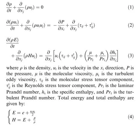
where e is the specific internal energy.The molecular stress tensor component and Reynolds stress tensor component are defined as:

2.2. SA turbulence model

The SA turbulence modelis a single equation model where a transport equation is solved for a variable^v related to the eddy viscosity. It has been widely used in engineering applications because it is less computationally expensive and more robust than the multi-equation models. It is defined as follows.

Turbulent eddy viscosity:

where Cis a model parameter,and ν is the kinematic molecular viscosity.

Transport equation:

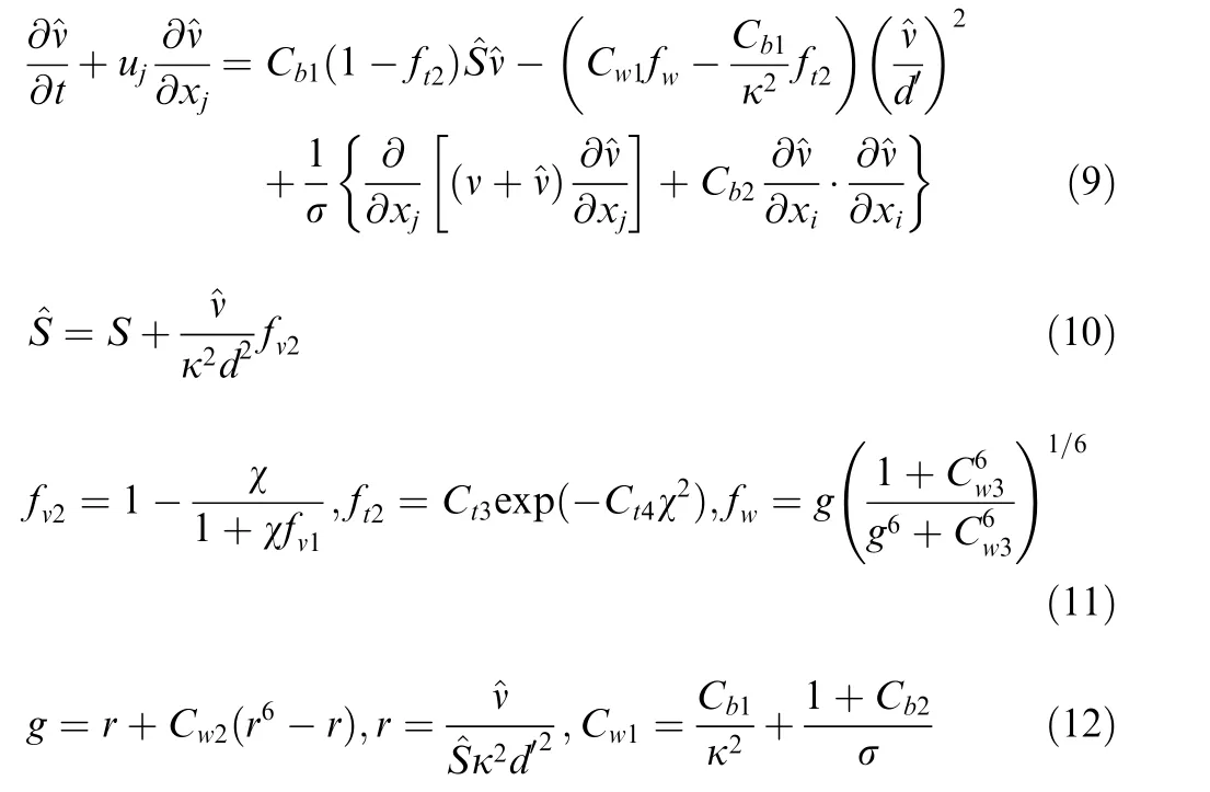
where S is the magnitude of the vorticity,^ν is the SA state variable,dis the distance to the closest wall,and C,C,σ,C,C, C, κ, Cand Care all the model parameters.

Referring to the previous works.7 parameters are considered in the calibration,namely C,C,σ,C,C,Cand κ . As with most turbulence models, the parameters of the SA turbulence model are determined by the model builder to match the characteristics of simple canonical flows.For example, the three parameters C, Cand σ are selected to match features of free shear flows, and the other parameters C, κ,Cand Care set according to the characteristic of a zeropressure-gradient boundary layer.Therefore,the original values(i.e.,nominal values)of these parameters may not be applicable to the supersonic jet interaction problem, and these parameters may need to be recalibrated. In order to carry out Bayesian parameter inference, the prior distributions of the parameters need to be given in advance. A uniform prior distribution is assumed for each parameter, because there is a lack of confidence in more informative priors for these parameters.According to Spalart and Allmaras,the prior range of parameter σ is restricted to[0.6,1].To make the solution variation obtained by prior propagation large enough to easily encompass the experimental data, the prior domain boundaries of C, C, Cand κ are set at ±50% of their nominal values. However, the prior ranges of Cand Care narrowed to ±25% of the nominal values to avoid nonphysical solutions. The nominal values and prior ranges of all parameters are given in Table 1.

where δis the Kronecker delta.

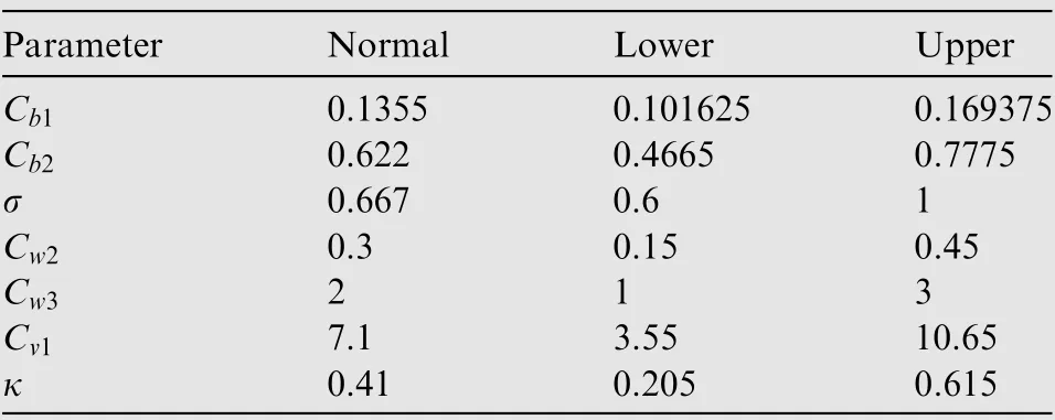
Table 1 Nominal values and prior ranges of all parameters.

3. Bayesian uncertainty quantification approach

In this section,the Bayesian uncertainty quantification method adopted in this work is briefly introduced, and more details can be found in the work of Sargsyan et al.

3.1. Bayesian calibration

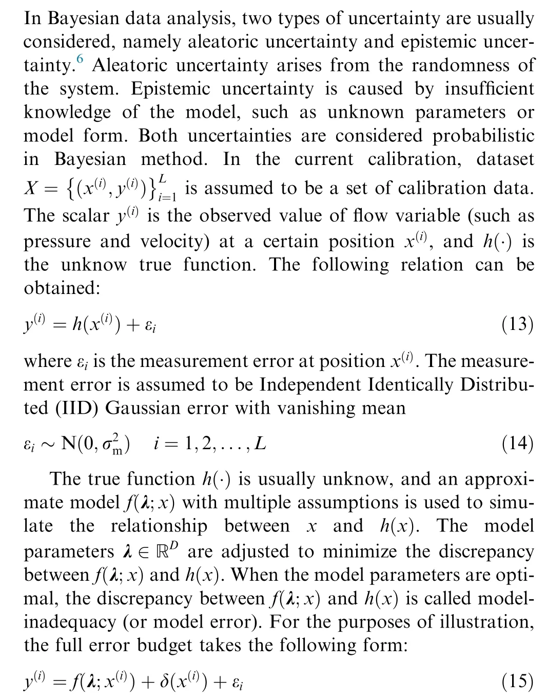
where δ（x）is the model-inadequacy term.Two scenarios are considered here for δ（x）. The first one is that modelinadequacy term is ignored, and the second one is that model error is embedded into the model itself.

To embed the model error,the original model parameters λ are augmented by a multivariate normal random variable as

where

The construction of likelihood functions is a key step in Bayesian inference, and four types of likelihood functions are applied here for comparison. Differences in likelihood functions can be considered as differences in statistical models.The descriptions of the likelihood functions are listed in Table 2.

The four types of likelihood functions are defined as follows:

M1 and M2:

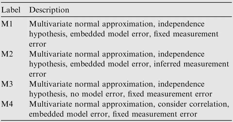
Table 2 Descriptions of likelihood functions.

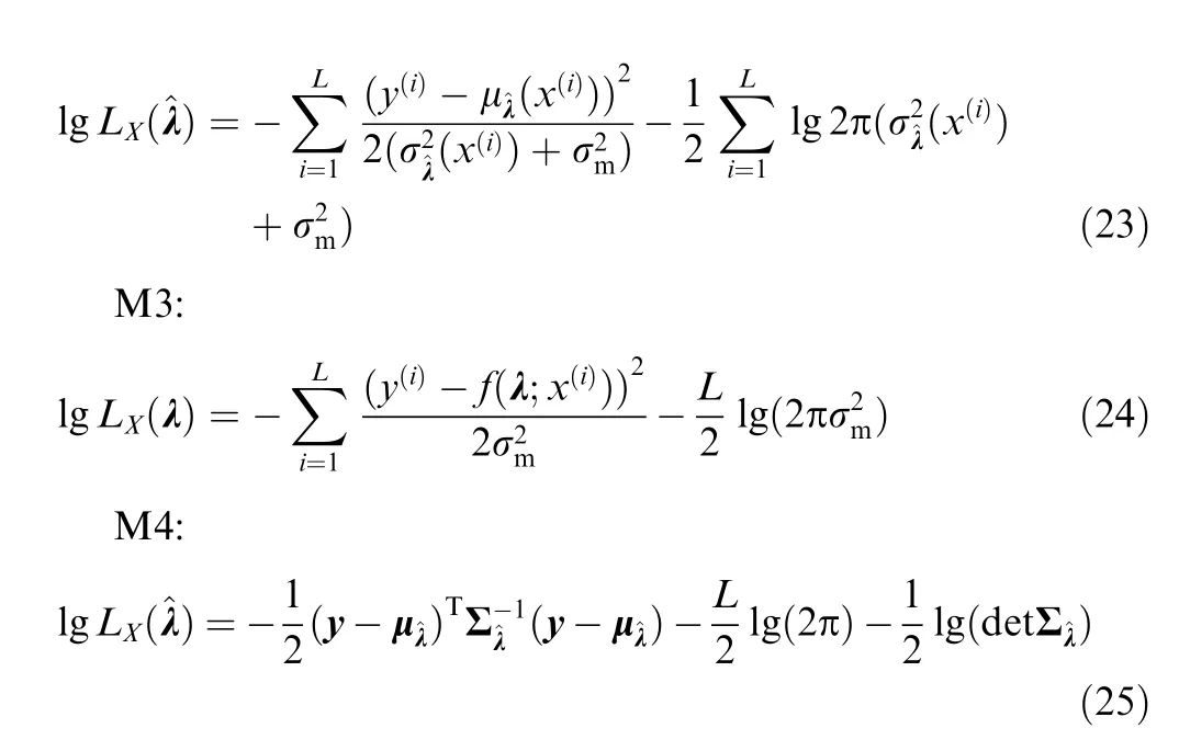
where y is a vector made up of y, μis the mean vector, and Σis the covariance matrix. The expressions of μand Σcan be found in Ref. 25. The fixed measurement error is set as the surrogate error in this work. It is difficult to accurately calculate the potential high-dimensional posterior, hence the adaptive Metropolis-Hastings Markov Chain Monte Carlo(MCMC) algorithmis employed to get posterior samples by sampling from the joint posterior probability distribution of the parameters.The marginal posterior distribution of each parameter can be obtained from the posterior samples by the kernel density estimation method.

3.2. Surrogate model construction

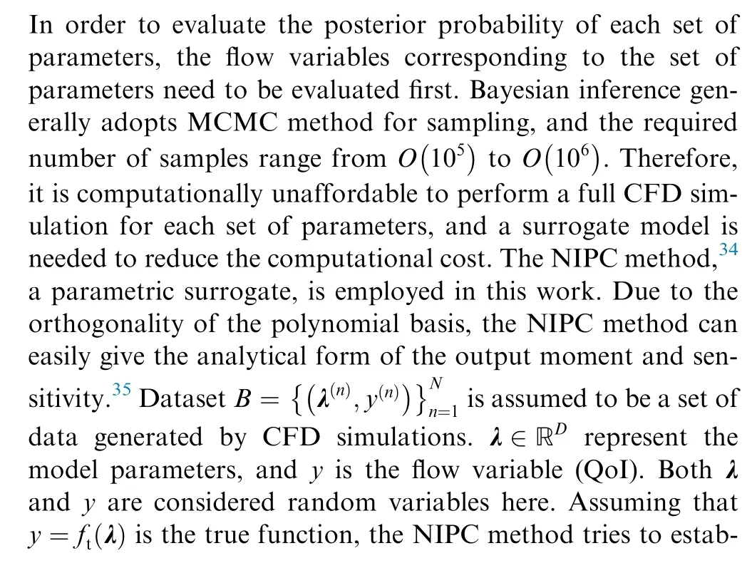
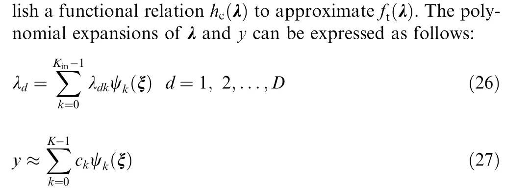
where λand care the coefficients that need to be solved,Kand K indicate the number of expansion items, and ψ（ξ）represents the basis function. Since the model parameters are assumed to be uniformly distributed, the Legendre Polynomials are utilized here. For the model parameters, first-order Legendre-Uniform expansion is adopted, and Eq. (26)becomes the following form:

where ξis IID uniform random variable on[-1,1],and[a,b]is the bound of λ. Eq. (27) can be written as

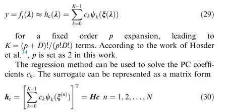
Table 3 Experimental conditions of slot injection experiments.

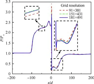
Fig. 1 Wall pressure distributions of different grids for Case 2.

where N is the number of training samples,and nis the oversampling ratio. The coefficients c can be solved by the leastsquares estimate. The closed-form solution can be written as follows:

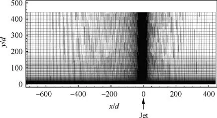
Fig. 2 Computational grid (grid resolution: 151 × 431).

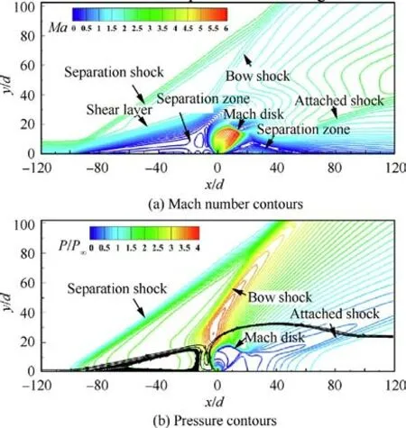
Fig. 4 Mach number contours and pressure contours near slot for Case 2.

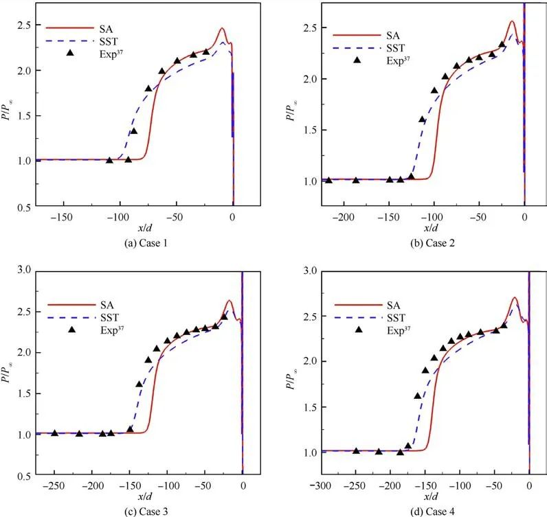
Fig. 3 Comparison of numerical simulation results of wall pressure with experimental data for all cases.

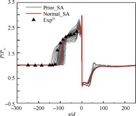
Fig.5 Wall pressure distributions of 108 prior samples for Case 2.

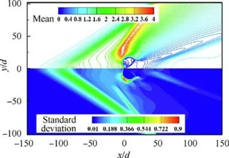
Fig. 6 Mean and standard deviation of pressure of 108 prior samples for Case 2.

The research of Hosder et al.showed that a better statistical approximation can be achieved when nis greater than 2.Therefore, n=3 is selected here. The total Sobol sensitivity index is defined as:

where {k（d）, k（d） ..., k（d）} is the list of indices of the expansion terms that include the dth dimension parameter.π（·） represents the probability density function of ξ. More details about surrogate models for uncertainty propagation can be found in Ref. 35.

4. Computational details

4.1. Experimental conditions

The supersonic jet interaction experiments conducted by Thayerare selected to verify the performance of SA turbulence model in such problems, and the experimental data are served as calibration data to recalibrate the parameters of SA turbulence model. In the experiments, the slot was 0.1270 m from the leading edge of the plate and the slot width d was 0.2032 mm. Nitrogen was injected perpendicular to the air. Experimental conditions are tabulated in Table 3. Pr is defined as the ratio of jet total pressure to free-stream static pressure, Maand Maare the Mach numbers of freestream and jet, Tand Tare the static temperatures of freestream and jet, and Pis the static pressure of free-stream.

4.2. Grid independency analysis and code validation

Grid independence analysis is necessary in numerical simulations to ensure sufficient solution accuracy. Case 2 is utilized to assess grid requirements. Three sets of grids with different resolutions(91×381,151×431 and 181×491)are generated,and the meshes near the wall and slot are refined to capture more flow details. The first cell spacing near the wall is set to satisfy y＜1.0. The wall pressure distributions simulated by the SA turbulence model for different grids are exhibited in Fig. 1. It can be found that the mesh resolution of 151 × 431 is sufficient to simulate the wall pressure, thus it is applied to all states in this paper. The computational grid is presented in Fig. 2. The jet is imposed at the position of x/d = 0.

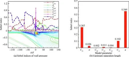
Fig. 7 Sobol indices of wall pressure and upstream separation length for Case 2.

The numerical simulation results of wall pressure are compared with the experimental data in Fig. 3. The results of SA and SST turbulence models are all given here.The parameters of both models are set to their nominal values. Since the upstream separation zone is the main research object in this paper,only the wall pressure distributions upstream of the slot are shown. For all cases,the SA turbulence model can predict the wall pressure in the high-pressure zone very well, but the predicted separation length is small.The separation length predicted by the SST turbulence model is close to the experimental value, but it performs poorly in the high-pressure area.

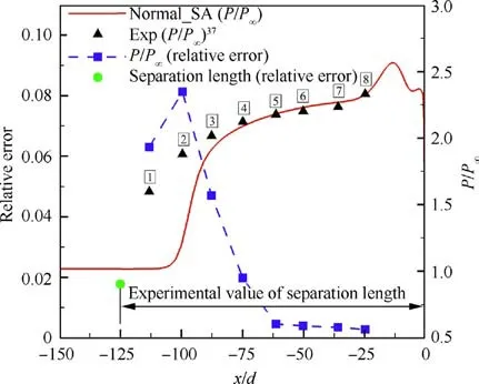
Fig. 8 Relative errors of surrogate model for Case 2.

4.3. Calibration details

To demonstrate the ability of Bayesian approach to get information from small datasets, only the experimental data of pressure upstream of the slot are used here. The experimental value of the upstream separation length can also be extracted from the experimental data of pressure. The upstream separation length is defined here as the distance between the point where the pressure rises for the first time and the slot center.The pressure data and the separation length can be respectively served as calibration data to infer the model parameters. The Latin Hypercube sampling method is employed to sample from the prior distributions. For each case, the training set contains 108 samples, the validation set contains 36 samples,and 144 full CFD simulations are performed to construct the surrogate model. The surrogate errors on the validation set are calculated to evaluate the model accuracy. For each calibration, 3×10posterior samples are generated by MCMC sampling. The samples in the first fifth of the MCMC chain are discarded to ensure convergence.To reduce the correlation between samples, one sample is reserved for every five successive posterior samples.Finally,the number of effective samples from each MCMC sampling is 48000. The posterior probability density distributions of model parameters are obtained from the posterior samples by the kernel density estimation method. The posterior uncertainty of the model parameters is propagated through the surrogate model to estimate the posterior uncertainty of QoIs. The MAP estimates of the model parameters can be regarded as the optimal values after recalibration, and the performance of the optimal values is evaluated by CFD simulation.

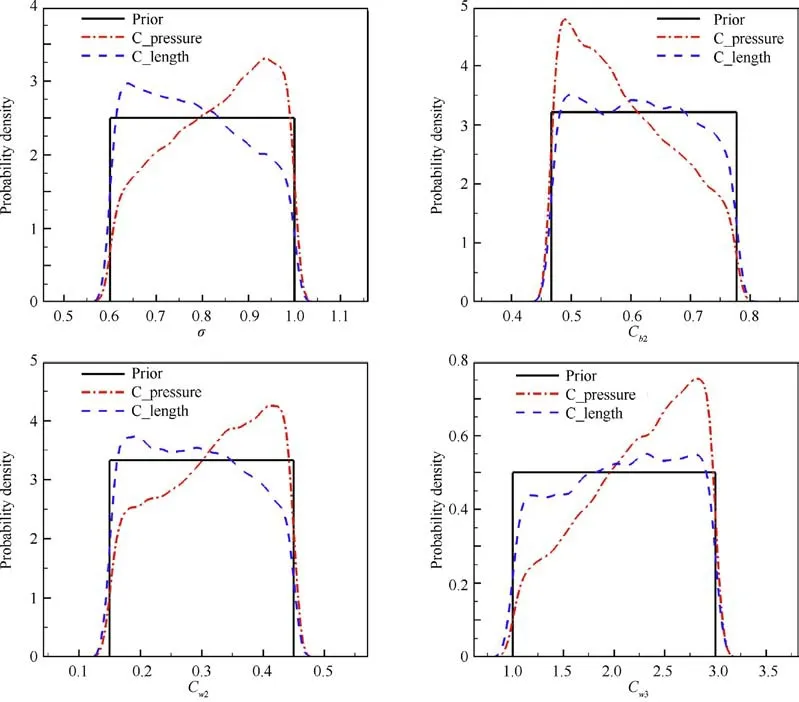
Fig. 9 Marginal posterior distributions of model parameters (σ，Cb2，Cw2，Cw3) for Case 2.

5. Results and discussion

5.1. Baseline results

Baseline results of transverse jet interaction at different pressure ratios are obtained using SA turbulence model with closure coefficients fixed at their nominal values. The wall pressure distributions of all cases are illustrated in Fig. 3.The Mach number contours and pressure contours of Case 2 are presented in Fig. 4.

All the crucial flow structures are clearly captured in Fig.4.The jet from the slot expands in the main flow, which causes the Mach number to rise gradually and the pressure to drop.Subsequently, a strong positive shock wave (known as Mach disk)is formed between the jet and the main stream to balance their momentum and pressure, and a bow shock appears upstream of the slot due to the obstruction of the jet. The bow shock forces the upstream boundary layer to separate under the adverse pressure gradient. The upstream separation zone makes the incoming flow deflect and a shear layer is formed between the incoming flow and the separation zone due to the difference in velocity. Meanwhile, a separation shock emerges in front of the upstream separation zone and intersects with the bow shock. After the supersonic incoming flow getting over the jet area,an attached shock occurs downstream of the slot to recover the velocity parallel to the wall and another separation zone is generated downstream of the slot.

5.2. Sensitivity analysis of model parameters

To identify the model parameters that can be informed by the experimental data,global sensitivity analysis based on variance is performed before Bayesian uncertainty analysis. The total Sobol index is utilized to represent the sensitivity of wall pressure and separation length to model parameters. The parameters with high sensitivity may yield informative posterior distributions, while the ones with low sensitivity may obtain posterior distributions that are less different from uniform prior distributions.

The uncertainties of all cases are similar, and thus only Case 2 is analyzed here. The wall pressure distributions of 108 prior samples for Case 2 are shown in Fig. 5. As can be seen,the wall pressure has great uncertainty in the two separation zones, and the uncertainty in the upstream separation zone is greater than that in the downstream separation zone.In the upstream separation zone, the pressure variation of 108 prior samples can easily encompass the experimental data,and samples with higher peak pressure have smaller upstream separation zone.The mean and standard deviation of pressure of 108 prior samples for Case 2 are exhibited in Fig. 6. The standard deviation represents the epistemic interval, and the mean is given to indicate the locations of the flow structures.For the pressure, the regions with larger epistemic interval are near the shocks.

Sobol indices of the wall pressure for Case 2 are given in Fig. 7 (a). The Mach number contours of the baseline result for Case 2 is also displayed in Fig.7(a)to indicate the locations of the flow structures. As can be seen from Fig. 5, the wall pressure in the two separation zones is of great uncertainty;hence only the Sobol indices in the two separation zones are discussed here.In the upstream separation zone,the first three parameters that contribute greatly to the uncertainty of wall pressure are κ, Cand C. In the downstream separation zone, the first three parameters that contribute greatly to the uncertainty of wall pressure are C, σ and κ. The difference of the Sobol indices between the upstream and downstream separation zones is closely related to many factors, including pressure, flow structures, etc. These factors combined lead to the complex different characteristics of Sobol indices.

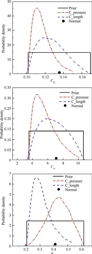
Fig. 10 Marginal posterior distributions of model parameters(Cb1，Cv1，κ) for Case 2.

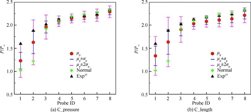
Fig. 11 Posterior means of pressure with estimated errors for Case 2.

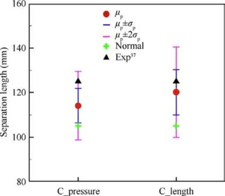
Fig. 12 Posterior means of separation length with estimated errors for Case 2.

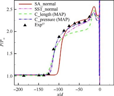
Fig. 14 Predictions using MAP estimates of model parameters for Case 2.

Sobol indices of the separation length for Case 2 are also exhibited in Fig. 7 (b). The three parameters, Cand Ccontribute more than 95% to the variance of the separation length.This is consistent with the results of sensitivity analysis of pressure in the upstream separation zone. Therefore, the model error is embedded into the three parameters κ, Cand Cin Bayesian analysis.

Fig. 13 Posterior variance decomposition of pressure for Case 2.

Table 4 Relative errors of predicted pressure for Case 2.

5.3. Calibration with different data

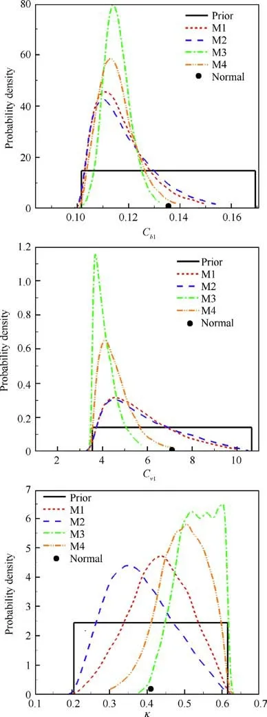
Fig. 15 Marginal posterior distributions of model parameters(Cb1，Cv1，κ) obtained by different likelihood functions for Case 2.

The wall pressure and the separation length are respectively served as calibration data to infer the model parameters. The likelihood function labeled as M1 is applied in this section.The calibration using pressure data is marked as C_pressure,and the calibration using separation length is tagged as C_length. All the calibration data for Case 2 are displayed in Fig. 8. The relative errors of the surrogate model for pressure and separation length are also exhibited in Fig.8.The relative error is defined as

where Yrepresent the wall pressure or separation length corresponding to the samples in the validation set, and Yrepresent the output of surrogate model. As can be seen, the relative errors of the surrogate model for pressure probes 4-8 and separation length are all less than 2%.The relative error for pressure probe 2 is the largest, but still less than 8.5%.Therefore, the accuracy of the surrogate model is sufficient for MCMC sampling.

The marginal posterior distributions of the model parameters for Case 2 are shown in Fig. 9 and Fig. 10. The posterior distributions of the four parameters (σ, C, Cand C) in Fig. 9 are not significantly different from the prior distributions, which indicates that the four parameters are not well informed by the calibration data. In Section 5.2, it is also proved that these four parameters contribute less to the total variance of the wall pressure in the upstream separation zone.In Fig.10,it can be seen that the parameters C,Cand κ are well informed by the data. For Cand C, values less than nominal are preferred, and this preference is stronger when pressure data are served as calibration data.For κ,the two calibration methods show different results. When the pressure data are used for calibration, values slightly larger than nominal are preferred. When the separation length is used, the result indicates that there is a high probability for κ to be less than the nominal value.

The posterior samples from MCMC sampling are used as inputs to the surrogate model to get the corresponding pressure and separation length. The posterior means of pressure and separation length are calculated as their Bayesian estimates. The total error including surrogate error, posterior uncertainty and model error is also estimated to represent the confident interval. The posterior means of pressure and separation length with estimated errors for Case 2 are shown in Fig. 11 and Fig. 12. μand σare posterior mean and posterior standard deviation.For C_pressure,the posterior means of pressure for probes 4-8 are not significantly different from the normal values and experimental values. The posterior means of separation length and pressure for probes 1-3 are better than the nominal ones but less than the experimental values. Except for probe 1 and the separation length, the σerror bands of pressure for other probes can cover the experimental values. For C_length, although the posterior mean of separation length is closer to the experimental value than the normal one and the result of C_pressure, the posterior means of pressure for most probes are further from the experimental values than the normal ones. Therefore, the calibration result of C_pressure is considered better than that of C_length.

The posterior variance decomposition of pressure for Case 2 is displayed in Fig. 13. It can be clearly seen that the total pressure variances of probes 1-3 are significantly higher than that of other probes in the two calibrations. Overall, the posterior pressure total variances of C_length are greater than those of C_pressure. The surrogate model adopted by the two calibrations is the same, and the same surrogate errors are generated in the two calibrations.The posterior uncertainties estimated by C_pressure are lower than those estimated by C_length.For the model errors,there are no significant differences between the two calibrations.

The predictions using the MAP estimates of the model parameters for Case 2 are illustrated in Fig. 14. The predictions in Fig. 14 are obtained by CFD solver, and thus no surrogate error is generated. The SA turbulence model with the MAP parameters obtained by the two calibrations can predict the separation length as well as the SST turbulence model does. However, the pressure in the upstream separation zone predicted by different methods is quite different. The result of the pressure prediction marked as C_pressure is very close to the experiment data and better than that of SST model.The pressure prediction marked as C_length performs poorly in the high-pressure region. To quantify the prediction error,the relative error of pressure for all probes is defined as

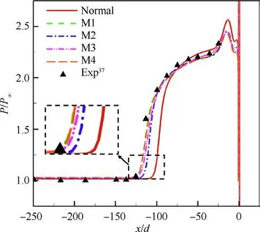
Fig. 17 Predictions using MAP estimates of model parameters obtained by different likelihood functions for Case 2.

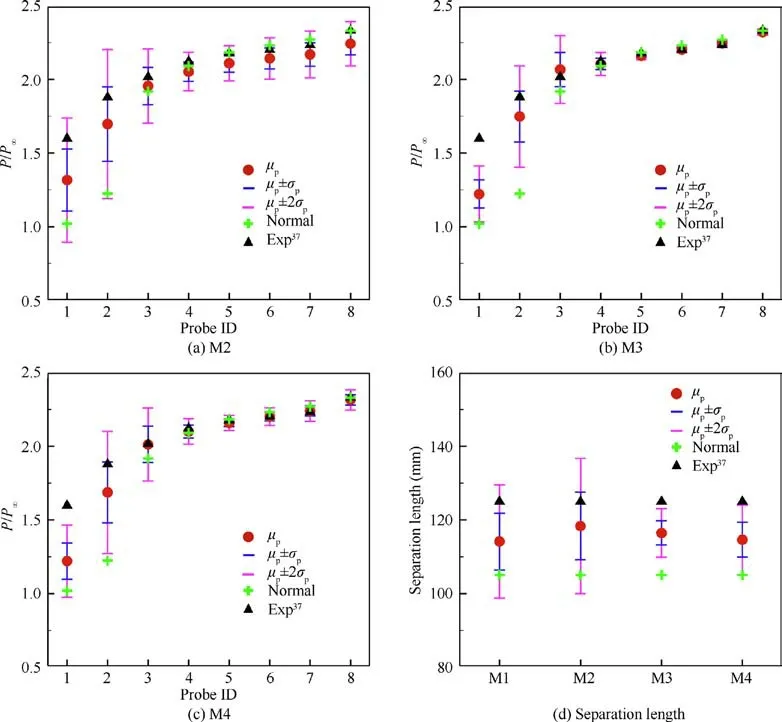
Fig. 16 Posterior means of pressure and separation length with estimated errors obtained by different likelihood functions for Case 2.

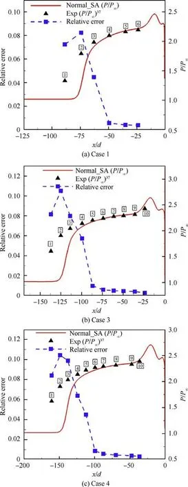
Fig. 18 Relative errors of surrogate model for Case 1, Case 3 and Case 4.

where Prepresent the prediction results of pressure for all probes,and Pare the experimental values of pressure for all probes. The relative errors of predicted pressure for Case 2 are given in Table 4.The relative error of SA model with nominal parameters is the largest,up to 14.99%.The relative error of SST model with nominal parameters is 4.56%,which is significantly lower than that of SA model. It is remarkable that the relative error of SA model with MAP parameters corresponding to C_pressure is only 2.95%. The results indicate that effective parameter calibration can improve the pressure prediction accuracy of SA model for two-dimensional jet interaction problem.

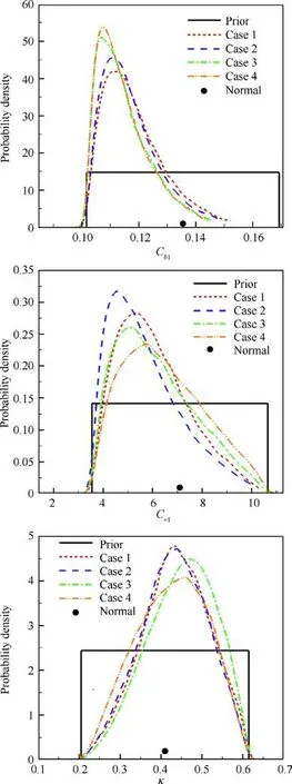
Fig. 19 Marginal posterior distributions of model parameters(Cb1，Cv1，κ) for all cases.

5.4. Calibration with different likelihood functions

As mentioned above, the construction of likelihood functions is the key step in parameter inference. In this section, the experimental data of wall pressure are used for calibrations.The marginal posterior distributions of the model parameters(C，C，κ)obtained by different likelihood functions for Case 2 are shown in Fig. 15. Only the parameters that are well informed by the experimental data are displayed here. For Cand C, all four functions show a preference for values smaller than the nominal ones. The sharp peaks of Cand Cgenerated by M3 and M4 indicate that there is less uncertainty in the parameter distributions inferred by the two functions. For κ, all functions except M2 show a preference for values larger than nominal.

The posterior means of pressure and separation length with estimated errors obtained by different likelihood functions for Case 2 are displayed in Fig.16.The result of M1 is the same as that of the calibration marked as C_pressure in Fig. 11. The posterior mean of separation length corresponding to M2 is the closest to the experimental value, but it performs worse than other functions in the high-pressure region. M3 and M4 make perfect pressure predictions in the high-pressure zone,but the estimated errors for the pressure of probe 1 and separation length are so small that the 2 σerror bands cannot cover the experimental values.

The predictions using the MAP estimates of the model parameters obtained by different likelihood functions for Case 2 are given in Fig.17.The MAP values of the parameters estimated by all functions show better performance than the nominal values. The MAP predictions of M1 and M4 basically coincide, and the MAP prediction of M2 for the separation point is worse than the other functions.

Since M1 can not only improve the prediction of wall pressure and separation length, but also estimate the total error reasonably, it is selected as the reference function and applied in most of the calibrations in this paper. The difference between M2 and M1 lies in the way of handling measurement error. M2 assumes that the experimental data have a large measurement error. The measurement error is considered an unknown variable that needs to be inferred together with the model parameters. Consequently, the overall error estimated by M2 is larger, and the pressure prediction based on the MAP parameters is also less consistent with the experimental data than other functions. M3 assumes that there is no model error, and the estimated total error only includes surrogate error and posterior uncertainty.Therefore,the marginal posterior distributions of C，Cand κ obtained by M3 have higher peaks,and the error bands estimated for wall pressure and separation length are narrower. M4 considers the correlation between the calibration data, which is more in line with the actual situation. Hence the posterior means of pressure estimated by M4 are closer to the experimental values than those estimated by M1. However, this correlation also weakens the ability of the pressure value at probe 1 to express information,making the error band estimated by M4 at probe 1 too narrow.

5.5. Calibration for different cases

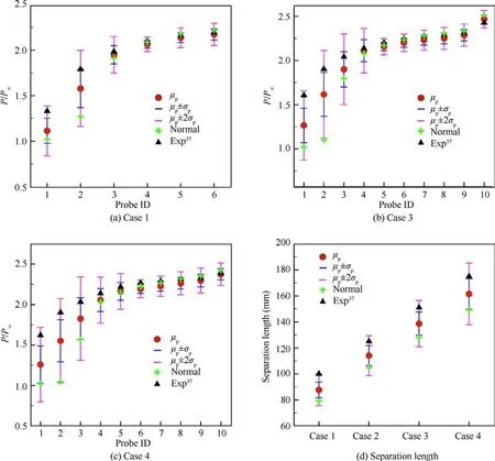
Fig. 20 Posterior means of pressure and separation length with estimated errors for all cases.

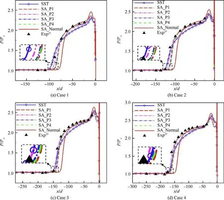
Fig. 21 Predictions using MAP estimates of model parameters calibrated in different cases.

To explore whether the parameters calibrated in one case are suitable for other cases,the calibrations in different cases(different jet total pressures) are carried out in this section. The likelihood function labeled as M1 is applied, and the pressure data are used for calibrations.The calibration results of Case 2 have been shown in Section 5.3,and they are partially omitted in this Section. The calibration data and surrogate errors for Case 1, Case 3 and Case 4 are presented in Fig. 18. The maximum relative surrogate error in Case 3 and Case 4 is slightly higher than that in Case 1 and Case 2,but not more than 11%.The calibration results for all cases are displayed in Fig.19 and Fig. 20. The similar posterior distributions of model parameters are obtained by calibrating in different cases,which proves the high similarity of flows in different cases.For Case 1,Case 3 and Case 4, the posterior means of pressure and separation length still exhibit better prediction performance than the normal ones, and the estimated 2σerror bands can better cover the experimental values. The predictions using the MAP estimates of the model parameters calibrated in different cases are exhibited in Fig. 21. SA_P1, SA_P2, SA_P3 and SA_P4 respectively represent the predictions made by the SA model with the MAP parameters calibrated by Case 1, Case 2, Case 3 and Case 4. The predictions of different MAP parameters in high-pressure region basically coincide, and they are all superior to the predictions of SST in high-pressure region.Different MAP parameters have slightly different predictions for the separation length, and they are all superior to the SA model with nominal parameters.Since the wall pressure distributions predicted by the four sets of MAP parameters have little difference in each case, it can be considered that the MAP values of parameters calibrated in one case are also applicable to other cases.

6. Conclusions

In this work,the embedded model error approach is applied to the Bayesian uncertainty analysis of SA turbulence model,and the parameters of SA turbulence model are recalibrated using the data from supersonic jet interaction experiment. The total Sobol index is calculated to represent the sensitivity of wall pressure and separation length to model parameters.Different calibration datasets and likelihood functions are investigated to compare the calibration effects. Furthermore, the model parameters are calibrated at different jet total pressures, and the applicability of the MAP values of parameters calibrated in one case to other cases is also investigated. The following conclusions can be drawn:

(1) The wall pressure has great uncertainty in the two separation zones, and the uncertainty in the upstream separation zone is greater than that in the downstream separation zone.

(2) Sobol indices exhibit different characteristics in the two separation zones. In the upstream separation zone, the first three parameters that contribute greatly to the uncertainty of wall pressure are κ, Cand C. In the downstream separation zone, the first three parameters that contribute greatly to the uncertainty of wall pressure are C, σ and κ.

(3) The parameters C, Cand κ can be well informed by the calibration data. The calibration result of C_pressure is considered better than that of C_length. Moreover, the relative error of the wall pressure predicted by the SA turbulence model can be reduced from 14.99% to 2.95% through effective parameter estimation.

(4) The posterior uncertainties of wall pressure and separation length estimated by different likelihood functions are significantly discrepant. The MAP values of parameters inferred by all functions show better performance than the nominal values. The MAP predictions of M1 and M4 basically coincide, and the MAP prediction of M2 for the separation point is worse than the other functions.

(5) The similar posterior distributions of model parameters can be obtained by calibrating at different jet total pressures. Since the wall pressure distributions predicted by the four sets of MAP parameters have little difference in each case, it can be considered that the MAP values of parameters calibrated in one case are also applicable to other cases.

The authors declare that they have no known competing financial interests or personal relationships that could have appeared to influence the work reported in this paper.

This research work is supported by the National Numerical Windtunnel Project, China (No. NNW2019ZT1-A03), and the National Natural Science Foundation of China (No.11721202).