An automatic isotropic/anisotropic hybrid grid generation technique for viscous flow simulations based on an artificial neural network

Png LU, Nianhua WANG, Xinghua CHANG, Laiping ZHANGa,,*,Yaong WU

a School of Information Engineering, Southwest University of Science and Technology, Mianyang 621010, China

b School of Intelligent Manufacturing Engineering, Chongqing University of Arts and Science, Chongqing 402160, China

c Stake Key Laboratory of Aerodynamics, China Aerodynamics Research and Development Center, Mianyang 621000, China

d Unmanned Systems Research Center, National Innovation Institute of Defense Technology, Beijing 100071, China

e School of Computer Science and Technology, Sichuan University of Science & Engineering, Yibin 644005, China

KEYWORDS Advancing front method;Advancing layer method;Anisotropic quadrilateral grid generation;Artificial neural network;Isotropic triangular grid generation;Machine learning

Abstract Based on the author’s previous research, a novel hybrid grid generation technique is developed by introducing an Artificial Neural Network (ANN) approach for realistic viscous flow simulations. An initial hybrid grid over a typical geometry with anisotropic quadrilaterals in the boundary layer and isotropic triangles in the off-body region is generated by the classical mesh generation method to train two ANNs on how to predict the advancing direction of the new point and to control the grid size.After inputting the initial discretized fronts,the ANN-based Advancing Layer Method(ALM)is adopted to generate the anisotropic quadrilaterals in boundary layers.When the high aspect ratio of the anisotropic grid reaches a specified value,the ANN-based Advancing Front Method (AFM) is adopted to generate isotropic triangles in the off-body computational domain.The initial isotropic triangles are smoothed to further improve the grid quality.Three typical cases are tested and compared with experimental data to validate the effectiveness of grids generated by the ANN-based hybrid grid generation method.The experimental results show that the two ANNs can predict the advancing direction and the grid size very well,and improve the adaptability of the isotropic/anisotropic hybrid grid generation for viscous flow simulations.

1. Introduction

In the past decades, Computational Fluid Dynamics (CFD)has become a hot research field. It has been widely used in the design, analysis, and optimization of aerospace, automobile, and thermal energy industries.As we have known, grid generation, also called ‘pre-processing’ in numerical simulation, is the first step in CFD and other numerical simulations.And grid quality will directly influence the accuracy of numerical results,so grid generation plays an important role in numerical simulations, hence the grid generation technique has become an important research branch in CFD.Despite decades of effort, high-quality mesh generation, especially for complex configurations, is still a grand challenge in the CFD community.

In the last 30 years,unstructured grid generation techniques have been obtained vigorous development due to the adaptability of complex geometries and the high efficiency of grid adaptation.Anyway,the‘pure’isotropic unstructured grids are not suitable for viscous flow simulations, because there is a very thin viscous layer in the boundary layer, in which the velocity gradient is very large.To capture the viscous effect accurately,more dense grids should be generated in the boundary layer.Since the flow in the boundary layer is strongly anisotropic,anisotropic grids are expected in this region.That is why we should generate isotropic and anisotropic mixed grids for viscous flow simulations, and anisotropic structured or semi-structured grids in the boundary layer and ‘pure’ isotropic unstructured grids in the off-body region are usually adopted in realistic numerical simulations.For the body-fitted anisotropic grid generation in the boundary layer,the Advancing Layer Method(ALM) is one of the most popular methods.For example,Bahrainian and Mehrdoostused the ALM to generate the grid of the boundary layer for complex geometry and solved the Navier-Stokes equation.Choi et al.used the ALM to generate structured grids near the solid wall and applied it to twodimensional (2D) and three-dimensional (3D) cases. Zhang et al.proposed a hybrid grid generation technique based on anisotropic tetrahedral agglomeration and a multigrid/parallel algorithm for turbulence flow simulations over 3D complex geometries. For a 2D case, for example, the basic idea of the ALM is as follows:(A)discrete the body surface with line segments and construct the initial advancing layer; (B) determine the advancing direction and distance at each grid point in the layer, and then generate the grid according to the topological relationship between two layers;(C)the grids are continuously generated in the computational domain with layer advancing until the length-width ratio reaches a specified threshold value.Of course,in the procedure of layer advancing,the intersection of advancing layers should be checked to avoid grid intersection with the existing layer.If the intersection of advancing layers occurs in some positions, the advancing procedure should be stopped locally.

The classical ALM needs to get the advancing directions at the points on the last layer,and check the convex and/or concave situation of the considered layer by iteration method to ensure the grid quality. Sometimes smoothing techniques should be introduced into the layer advancing procedure.Therefore,these operations will result in low efficiency of grid generation.To get a better grid quality,a lot of tedious and time-consuming manual operation is also required,as a user using a grid generation software with a Graphic User Interface(GUI).Therefore,many scholars have done a lot of research on how to improve the grid generation efficiency of complex shapes.

In recent years, with the rapid development of science and technology, Artificial Intelligence (AI) technology is widely used in many fields such as image processing, speech recognition, UAV flight control,intelligent recommendation,machine translation, and other industries. Of course, AI technology has also been preliminarily applied in CFD studies.Sun and Andeveloped a data-driven turbulence model with low complexity acting as an algebraic turbulence model to estimate the turbulence eddy viscosity for Reynolds Averaged Navier-Stokes (RANS) equations. On the other hand, grid generation is an important part of CFD applications, so three main types of AI methods(connectionism,symbolism,behaviorism) have been applied in grid generation in the past few years. Symbolism is an intelligent simulation method based on logical reasoning to simulate the intelligent behavior of human beings. As the most influential symbolism method,Reichert et al.introduced an expert system to 2D grid generation. Essentially, this method proposed an expert system instead of geometric rules in grid generation, and each angle of the polygon is analyzed to determine which grid will be generated and the location of new points.However,sometimes an overly precise mathematical description may not be able to achieve the ideal effect, so Kwok and Haghighiproposed a fuzzy logic method to generate the finite element grid generation.The finite element expert heuristic knowledge,experience,common sense, and other special methods were incorporated into the knowledge base of the fuzzy system. On the connectionism side,Ahn and Leeproposed a finite element grid generation method based on a self-organizing neural network. In this method, the neural network nodes are connected with the actual point clouds, and the grid generation is completed through continuous iteration until the nodes of the neural network match with point clouds.Yao et al.proposed an ANNbased element extraction method for automatic grid generation,and the ANN was adopted to replace an expert database for pattern recognition.For the behaviorism AI approach,it is mainly used for grid quality optimization.For example,Yilmaz and Kuzuogluproposed Particle Swarm Optimization(PSO)to optimize the quality of the hexahedral mesh, which solved the problem of the poor effect of the Laplacian mesh smoothing algorithm in concave regions. The above AI methods have improved the automation and intelligence level of grid generation.However,none of these studies has solved the problem of isotropic and anisotropic mixed grid generation. So in this work, based on our previous study,we try to adopt the ANN-based machine learning method combined with the classical ALM and Advancing Front Method (AFM) to improve the adaptability of the hybrid grid generator system.

As we know,the anisotropic quadrilateral grids with a high aspect ratio are necessary for viscous flow simulations in the boundary layers, but unnecessary in the off-body regions. To speed up the grid generation, the AFM is often used to generate isotropic triangular grids in these regions.To control the grid size during the front advancing process and to obtain a smooth grid distribution, it is usually necessary to establish a background grid. A large number of researchers have done in-depth research on the AFM.However, this method takes much computation time to determine the grid size by using the background grid method due to the timeconsuming donor cell searching procedure. So here, based on our previous work,we propose a control strategy to predict the grid size based on the ANN.

In this study, the main ideas of isotropic and anisotropic hybrid grid generation for viscous flow simulations include two points:(A)the first ANN is used to predict the advancing direction (including multiple advancing directions at sharp convex corners) and relative step size factor of the new point generated by the ALM;(B)another ANN is applied to predict the grid size during AFM.The rest of this paper is organized as follows: in the Section 2, the grid generation technique based on two ANNs is presented in detail, including the improved ALM based on the ANN, the training data set extraction method, the ANN structure, and how to predict the grid size.In Section 3, some typical 2D geometries, including the NACA0012 airfoil, a fighter with a store, and the 30P30N three-element airfoil are tested to validate the capability of the isotropic and anisotropic triangular grid generation algorithm with the ANNs. Then the CFD simulations are carried out on grids generated by the ANN-based hybrid grid generation method and compared with wind tunnel experimental data. Finally, Section 4 summarizes the work in this paper,and the prospect for future work is discussed.

2. Isotropic and anisotropic hybrid grid generation algorithm based on ANN

2.1. Basic idea of isotropic and anisotropic hybrid grid generation

The general procedure of 2D hybrid grid generation based on ALM and AFM can be listed as follows:

(1) Discrete the body surface with line segments according to the geometric feature. In the region with a small curvature radius, the discrete segments should be refined properly to capture the accurate geometric feature.

(2) Carry out the ALM layer by layer to generate the anisotropic grids normal to the solid wall. Here anisotropic quadrilaterals could be generated with a defined growth ratio. The normal size of the first layer is defined by the Reynolds number of the incoming flow.

(3) Return to Step (2) until the fronts intersect with others or the aspect ratio meets the specified threshold value.If so, the advancing procedure is stopped locally.

(4) After generating the anisotropic grid in the boundary layer,the outer boundary of the anisotropic grid is treated as the initial advancing front, and then the AFM is carried out to generate the isotropic grid in the off-body regions.

(5) Grid smoothing, grid quality analysis, and grid output.

During the ALM and AFM steps, the advancing direction,relative step size factor, and grid size are three important parameters to control the grid quality and distribution. Here in this work, different from the classical control strategy, we try to introduce ANN-based methods to control these parameters. The purpose is to make the grid generator more intelligent. So in the next sub-sections, we will introduce how to train the ANNs and how to use the ANNs to generate the anisotropic and isotropic hybrid mesh.

2.2. ANN-based advancing layer method

In this section,we will introduce the ANN-based ALM to predict the advancing direction, relative step size factor, and the angle between the advancing vectors.

2.2.1. Brief review of traditional ALM

The ALM generates a layer of structured/semi-structured and anisotropic cells by advancing the initial layer (the discrete boundary, line segments) into the computational domain. In the previous section, the general idea has been introduced briefly, and the specific steps and implementation methods are listed as follows:

Before the layer advancing begins, the solid wall is discretized as line segments to construct the initial fronts, and the data information of the fronts is stored in a linked list.

(1) The advancing direction of each point is determined,which is one of the key issues for the ALM. The direction of each point is taken as the average of the normal direction of adjacent fronts in the same layer, which can be defined as

where nis the advancing direction of the grid point p,Nis the total number of adjacent fronts,and nis the outer normal vector of Front i (pointing into the computational domain).

However, in the cases of concave and/or convex angle, the advancing direction needs to be smoothed by Laplace iterative algorithms to improve the grid quality,as shown in

where t represents the smooth iteration step, and ω is the weighted coefficient of the normal vector of the neighbors of point p.

(2)In the process of the ALM implementation,if the geometry has a large convex angle,it is necessary to adopt the multidirection advancing technique, which will also be discussed in Section 2.4.

(3) After determining the advancing direction(s) of each point, the advance distance of the point needs to be determined. Exponential growth is a common method for advancing distance, which can be written as

where δand δrepresent the advancing distances of Layer l and Layer 0, respectively. The size of Layer 0 depends on the Reynolds number of the incoming flow. β is the grid size growth rate, which depends on the flow state, e.g., laminar or turbulent. In general, for laminar flow, β is set to 1.1-1.25, while for turbulent flow, β is usually less than 1.1.

(4) When the advancing direction and distance are determined, the new point can be inserted into the computational domain, and the formula is as follows:

where rand rrepresent the coordinates of Layer l and Layer (l + 1), respectively.

(5) The intersection checking of the new and old grids.If a new cell intersects with other new or old cells,the new cell will not be added to the cell list,and the advancing process is set to stop locally.

2.2.2.An ANN-based ALM:Algorithm and system architecture

The classical ALM needs to determine the advancing direction and distance, and this algorithm can obtain an excellent performance in the case of simple geometry. However, the iterative optimization technology is adopted when dealing with complex geometries, and this will be a time-consuming procedure.As well known,the ANN has unique advantages in classification and prediction,and this is the reason why it has been a research hotspot in recent years, even in the CFD community.So in this work, an ALM based on an ANN is developed to solve the above problems, and the detailed description of this approach is shown in Fig. 1.

2.2.3. Automatic collection of training samples

In this work, the ANN is used for data fitting and prediction.The first step in the application of machine learning is to make a training data set,so the classical ALM is used to generate the initial training grids as the training data set. The adjacent points of the left and right endpoints of a reference front are taken as the training input. The reference fronts are the grid edges on the advancing layer.The fundamental purpose of this ANN is to obtain the direction of the advancing point according to the situation of the connection points and edges, and thus to replace the classical iterative algorithm.

Theoretically,there are many left and right adjacent points for an advancing point. However, the far points have little effect on the new grid advancing direction.To extract training data quickly and conveniently, in this work, only the points connected immediately with the advancing point are taken as inputs. As shown in Fig. 2(a), the adjacent point to the left of point Pis Pand the right adjacent point is P. The ANN belongs to supervised learning, so its input data need to be labeled. Taking point Pas an example, the training input data set is the coordinates of P, P, and P, and the input data labels are the vector PPin Fig. 3(a), the relative advancing step size factor and the angle ∠PPP, as shown in Fig. 2(b). The vector PPis the mean normal vector of Front PPand Front PPas the advancing direction. The angle ∠PPPis related to the number of multi-direction advancing.It should be noted that the labels of the input data are also the outputs of ANN.

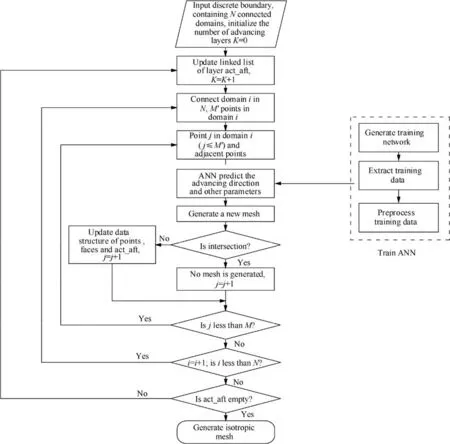
Fig. 1 Flowchart of an ANN-based ALM.

Fig. 2 Normal vector of faces and advancing direction of points in 2D case.

The training data for various conditions will be collected to improve the prediction effect of the ANN.After sufficient iterations, the weights of ANN will converge, indicating that the training process of the ANN is completed.When the unlabeled input data are fed into the ANN, the output of the ANN can accurately predict the parameters required for mesh generation.

Algorithm 1 presents the training data extraction method from an example grid. Using Algorithm 1, we can automatically extract the training data set from a given grid.The training data set contains input features and labels as shown in Fig. 3.

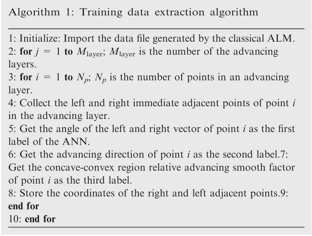
Algorithm 1: Training data extraction algorithm 1:Initialize:Import the data file generated by the classical ALM.2: for j = 1 to Mlayer; Mlayer is the number of the advancing layers.3: for i = 1 to Np; Np is the number of points in an advancing layer.4: Collect the left and right immediate adjacent points of point i in the advancing layer.5: Get the angle of the left and right vector of point i as the first label of the ANN.6: Get the advancing direction of point i as the second label.7:Get the concave-convex region relative advancing smooth factor of point i as the third label.8: Store the coordinates of the right and left adjacent points.9:end for 10: end for

2.2.4. Standardization of training samples

The standardization processing of the training sample data is a basic work for machine learning, and different evaluation feature data tend to have different dimensions and dimensional units, which will influence the result of data analysis. To eliminate the dimension influence between feature data, the training data needs to be standardized. After the standardized processing of the original data, each sample feature data is in the same order of magnitude, which is suitable for comprehensive comparative evaluation.

As shown in Fig. 4, the normalization process contains translation, scaling, and rotation. The start point Pand the endpoint Pof the front are used for normalization processing,and the coordinate values are(0,0)and(1,0)respectively after the final processing.An example sub-set of the training data of the ANN is shown in Table 1, and the normalized data are shown in Table 2.It should be noted that the normalized data needs to be de-normalized in the grid generation process.

2.2.5. Structure of ANN model

The essence of an ANN can be understood as the process of obtaining the best solution through constant iterative optimization of parameters, which is also a process of negative feedback. The Back-Propagation (BP) neural network is a multi-layer neural network with the input layers,hidden layers,and output layers. The input signal transfers through the forward path, and the error signal feeds back through the backpropagation. The main idea of ANN training is to obtain the minimum mean square deviation between the actual output and the ideal output by changing its weights constantly through the gradient descent method. In other words, ANN training is the process of error back-propagation to correct its parameters.Because of its strong data fitting and prediction ability,in this work,the BP neural network is adopted to automatically predict the position of the advancing point.

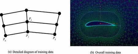
Fig. 3 An example of training grids and training data extraction of an ANN.

Fig. 4 Normalization processing of input training data.

Table 1 Unnormalized training data set of one front.

It is generally believed that the more complex the neural network structure is, the more layers and nodes there are,and then the ANN tends to have better network performance and generalization capabilities. However, the disadvantages are the cost of training time and model overfitting. Therefore,it is crucial to select the ANN model suitable for the prediction of ALM direction and advancing distance. Generally, the first choice is a three-layer ANN which contains a hidden layer,an input layer, and an output layer. The number of nodes in the hidden layer can be adjusted appropriately. Increasing thenumber of nodes in the hidden layer is easier to achieve than increasing the number of hidden layers. Theoretically, it has been proved that a three-layer neural network containing a hidden layer can approximate any nonlinear function with arbitrary precision, and the number of neurons in the hidden layer can be adjusted arbitrarily.

Table 2 Normalized training data set of one front.

If the number of nodes in the input layer is 6, and the output layer is 4,the number of nodes of the hidden layer is determined as follows:

where m,n,and l are the numbers of nodes of the hidden layer,input layer, and output layer, respectively. α is a constant between 1 to 10. So the number of nodes of the hidden layer can be determined to be 8. It is also important to note that the number of nodes in the hidden layer must be less than the sample number. As shown in Fig.5,the input signal is the vector containing the coordinates of three points, P, P, and P,the output[d,d]is the advancing direction of Pthe signal flag1 is the relative advancing step factor in the concaveconvex region and flag2 is the angle of two vectors.

As shown in Fig. 6, we develop an ANN to predict the advancing direction, the relative advancing smooth factor in the concave-convex region,and the angle between the vectors,and the process can be described as follows:

Collect the training samples and design ANN architecture.The inputs of the ANN predict system are the coordinates of the three points,P,P,and P.The method to obtain training data has been explained in Sections 2.2.3 and 2.2.4.

(1) Set the weight coefficients of interneuron connection to the random numbers from-1 to 1(‘‘-1”represents a negative correlation, and ‘‘1” represents a positive correlation). To improve learning efficiency, the learning rate is relatively high at the beginning of training, and it is necessary to reduce the learning rate after a certain stage of learning. Otherwise, the output will oscillate and thus lead to non-convergence. In this work, we set the learning rate from 0.1 to 0.0001.

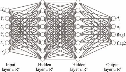
Fig. 5 Schematic diagram of ANN structure for ALM.

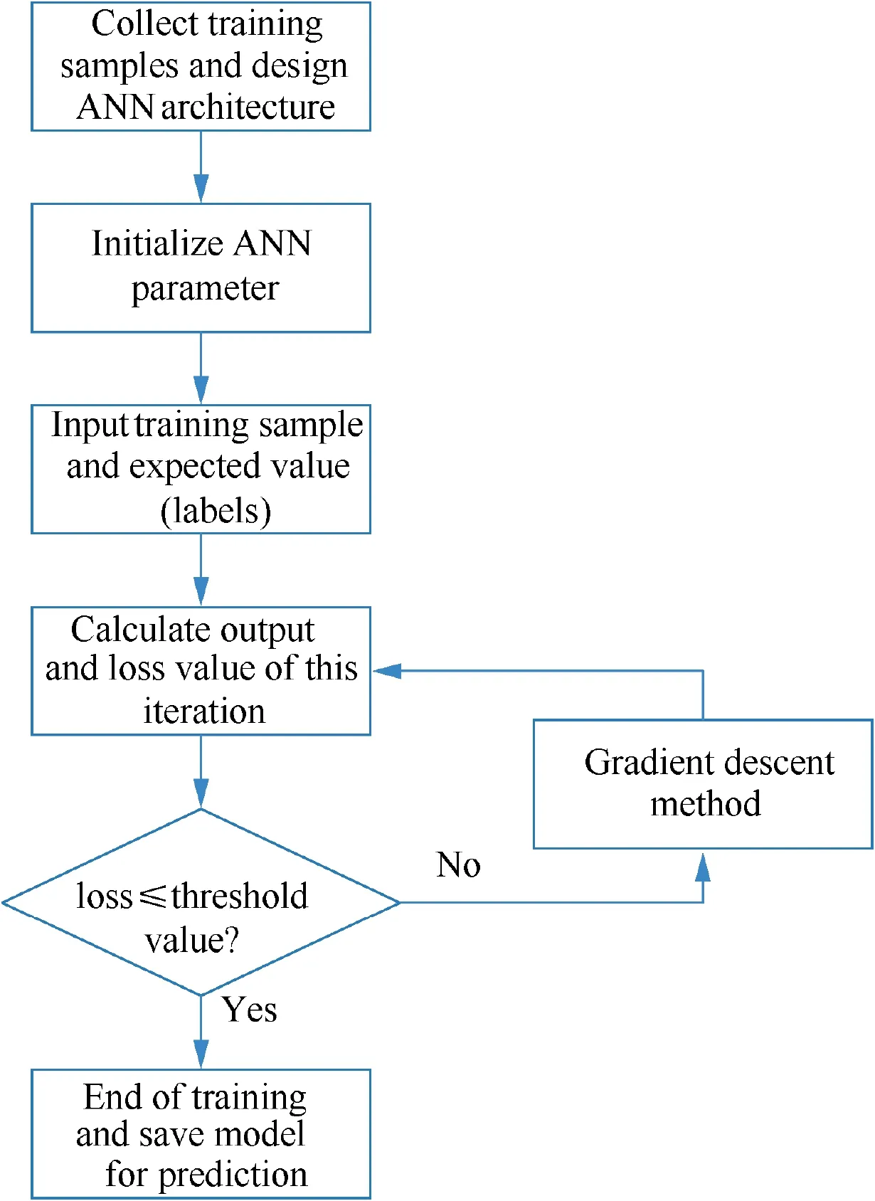
Fig. 6 Flowchart of advancing direction and angle prediction neural network.

(2) The output vector Y contains the predicted advancing direction and the angle,and the label value is T.Then the loss function of the ANN is defined as

(3) If loss≤loss, the training results are convergent and the ANN model is saved;otherwise,the weight coefficient of neurons is optimized by the gradient descent method.

where η is the learning rate and wis the neuron weight of the ANN.

(4)To improve the nonlinear fitting ability of the ANN,the activation function is adopted.Otherwise,the output of a multilayer neural network is still only a linear combination. Here,the sigmoid function is used as the neuron activation function of the output layer. The sigmoid function is defined as

2.3. An ANN-based grid size control in off-body regions

The design of the ANN for predicting grid size is similar to the method which is introduced in Section 2.2. Here we just give the input, output values, and the structure of the ANN.

2.3.1. Classical control method of grid size

The distribution of the initial grid is usually realized by human intervention in the grid generation, and many grid generation systems provide interactive tools to assist engineers to complete this process quickly. Generally, there are four methods of grid size distribution as follows:

(1) Use a global grid size to define a uniform grid distribution,which is a numerical constant,and all grid sizes are equal to this value.

(2) The density of the whole grid size is controlled by the density of the points on the boundary and the grid size inside the region is determined by a certain size transition method.

(3) The grid size distribution is controlled by the background grid which is created by the user manually or semi-automatically.

(4) The local element density is controlled by the grid source, especially for the grid generation in the boundary layer.

In this work, the second method is adopted, and an ANNbased approach is developed to control this transition through a large amount of training data.

2.3.2. Collection of characteristic data of ANN

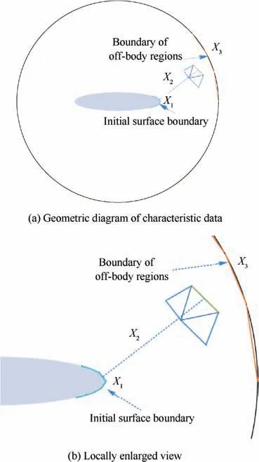
Fig. 7 Input training characteristic data of ANN.

In the process of grid size prediction, the first step is to define the input characteristic data of the ANN. As shown in Fig. 7,the grid size is related to the distance from the grid element to the nearest boundary layer, the length of the front in the boundary layer, and the boundary of off-body regions. The desired grid size is generated by classical AFM. According to the requirements of the system, a BP neural network for grid size prediction is designed as shown in Fig. 8. The ANN has three layers, there are three neurons in the input layer to receive the input characteristic data, and the output layer y represents the predicted grid size.

2.3.3. Test for ANN

After the training data are normalized, which should be divided into the training set and test set. The training data are fed into the ANN, and the gradient descent method is used for continuous iterative convergence until the loss reaches the preset threshold value. As shown in Fig. 9, when the step reaches 15000, the loss value converges to 0, which shows that the ANN can meet the requirement of the grid step size.

2.4. Grid optimization techniques

The long-term practice has shown that the grid quality dominates the accuracy of numerical simulation. In the CFD community, the basic requirements of the grid are smoothness,orthogonality,and reasonable grid distribution.However,there is no uniform standard to define the quality of the hybrid grid. Following the practical experience, some common optimization techniques are used in this work to improve the grid quality.

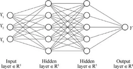
Fig. 8 Schematic diagram of ANN structure for grid size prediction.

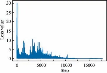
Fig. 9 Loss value of ANN-based AFM vs training step.

2.4.1. Multi-direction advancing technique

In the process of generating body-fitted mesh by the ANNbased ALM, the advancing direction is distorted seriously at a convex angle as shown in Fig. 10 (a), which does not reach the quality requirements of mesh orthogonality. The multidirection advancing technique is a suitable approach to solve this problem, see Fig. 10(b).

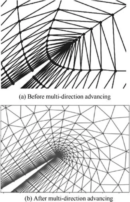
Fig. 10 Multi-direction advancing technique.

The multi-direction advancing technique can be divided into two steps. Firstly, the convex angle is detected by the geometry considered. In this work, we use the ANN method to identify it. Secondly, several advancing direction vectors are designed in the convex part, the number of the advancing direction is determined by the angle detected by the previous step, and the grids are generated by the classical ALM.

2.4.2. Smoothing the advancing step in concave and convex regions

Similar to the multi-direction advancing technique, this advancing step smoothing technique is also applicable to the ANN-based ALM. In the case of complex boundary conditions, the concave and convex angles may exist. When the ALM is used to generate viscous layer mesh, it may result in grid intersection in the sharp concave area and thus makes the grid invalid. Through a lot of experimental analyses, the mesh quality can be improved by increasing the step size at the concave corner and reducing the step size at the convex corner. The relationship between the curvature and the step size is given as

2.4.3. Diagonal transformation

In the process of the isotropic grid generation by the ANNbased AFM, the inner angles of some triangles may be very small, and those triangles do not meet the quality requirements. If the diagonal AC of quadrilateral ABCD is replaced by BD as shown in Fig.12,it is clear that the quality of the triangular grid is improved. The Delaunay criterion is adopted here to determine whether or not to exchange the diagonal.

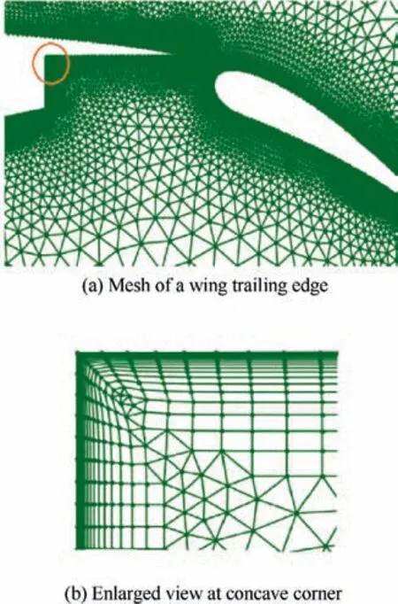
Fig.11 Smoothing the advancing step size in local concave area.

2.4.4. Node relaxation based on spring analogy

After the diagonal transformation, the node relaxation approach is adopted to further improve the grid quality.As shown in Fig. 13, Point P is moved to Pby the spring analogy technique. The essence of this method is to move the position of each internal point in the grid to the center of the polygon around it to reach a balanced state, just like a spring system, as shown in

where (x,y) is the coordinate of one node, and N is the total number of points connected to node i.

It should be noted that the first two techniques are applied to the anisotropic gird optimization generated by the ALM,while the last two techniques are applied to the isotropic gird optimization generated by the AFM. In this paper, the ANN has been introduced into the first two approaches to improve the mesh generation efficiency and quality.

3. Results and analysis

To demonstrate the capability of the present ANN-based hybrid grid generation method,some typical cases will be illustrated in this section. The software development environment is as follows: Ubuntu18.0.4, TensorFlow-1.2.1, Python-3.6,and the module ‘matplotlib’ for grid visualization. The hardware platform is a notebook computer with a 4-core processor and 8 G memory.

3.1. NACA6412 airfoil

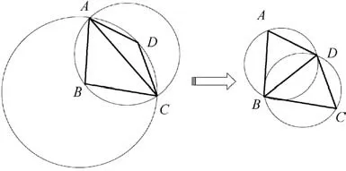
Fig. 12 Diagonal transformation.

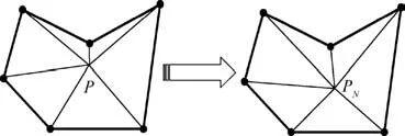
Fig. 13 Node relaxation based on spring analogy.

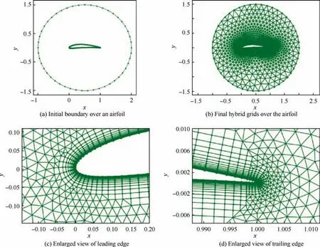
Fig. 14 Hybrid grid over an airfoil.

Fig. 14 shows the quadrilateral/triangular hybrid grid over a NACA6412 airfoil, which is a typical benchmark case. This grid includes 5665 nodes and 5650 cells, including 2782 anisotropic quadrilateral cells in the boundary layer and 2878 isotropic triangles in the off-body region. To discretize the airfoil more accurately, more grid points are located in the leading-edge and trailing-edge regions of the initial boundary.As shown in Fig.14(c)-14(d),the grid sizes of these two regions are relatively small, and the transition from the anisotropic grids to the isotropic grids is very smooth. Due to the sharp trailing edge, the multi-direction advancing technique is applied in this region, as shown in Fig. 14(d), so the grids in this region are very smooth, too. In the following figures, the values of abscissa and ordinates are dimensionless, which are used to show the positions of the grid points.

3.2. A fighter with a released store

This configuration consists of two objects, a fighter and a released store,which is more complicated than the NACA6412 airfoil. There are two concave corners less than 90° in the initial boundary.Fig.15 shows the grids over the joint configuration. The connection between the anisotropic grids and isotropic grids is natural and smooth(Fig.15(b)-15(d)).Based on the idea of grid distribution control,the grids near the noses and the trailing edges of the fighter and the store are refined to get a more precise description of the geometry (Fig. 15(b)-15(d)). In the regions with a small curvature radius, such as the inlet and the vertical tail, the grids are also refined to capture the geometry more accurately. For anisotropic quadrilateral mesh generation, when the ratio of the length over the width is approximately equal to 1.0, it should be stopped locally in the advancing procedure.In the regions of concave and convex corners, the advancing steps are factored by the relative advancing step factor,so the quadrilateral cells in these regions are very smooth (Fig. 15(d)).

3.3. 30P30N three-element airfoil

The last case is the 30P30N three-element airfoil, which is a typical test case for the taking-off or landing of an aircraft.The final hybrid triangular grids are shown in Fig. 16, including 32,240 cells (25192 quadrilaterals and 7048 triangles),61,340 faces, and 29,098 points. Similar to the previous two cases,the grids are refined near the leading edges and the trailing edges of each component of the three-element airfoil where the curvature varies greatly. To eliminate the influence of the far-field boundary, the radius of the far-field circle reaches 20 times the length of the airfoil chord length, and the densest part of the leading edge reaches 0.0001. It is particularly worth mentioning that the multi-directional advancing technique is applied for the sharp trailing edges (Fig. 16(c)-16(g)), and the number of advancing directions is different because the angles are not equal. In this work, the ANN is adopted to predict the number of multiple advancing directions.

3.4. Grid quality evaluation

In this section, the quality assessment of anisotropic and isotropic grids is discussed separately because of their essential differences.

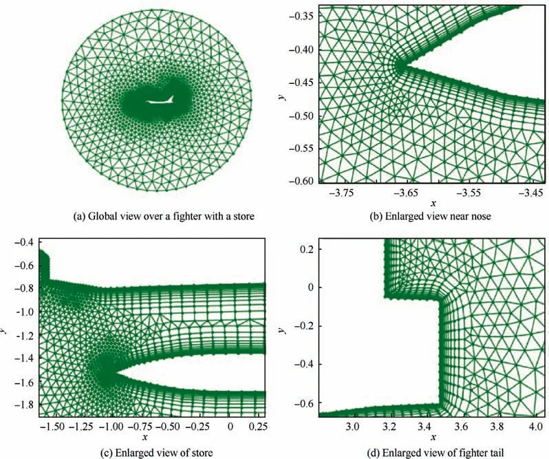
Fig. 15 Hybrid triangular grids over a fighter with a released store.

The quality coefficient of the isotropic grid is usually determined by the ratio of the radius of its inscribed circle and circumscribed circle,and when the ratio is 0.5,the triangle has the best quality(equilateral triangle).This approach can be simplified further.So another triangle quality coefficient, the isotropic grid shape index q, defined by Eq. (11), is used in this work.

where Sis the area of the triangle, and a, b, and care the three edge lengths of the triangle.To ensure 0 ≤q ≤1,the normalized coefficient, k=4■■■3. When the triangle is equilateral,q=1,while in the case of three points being collinear,q=0.To calculate the area of a triangle directly, Helen’s formula is used as follows:

According to Eq. (11) and Eq. (12), q can be expressed as

Then, we will check the quality of the generated grids.Table 3 lists the grid quality coefficient distributions of the three cases in Sections 3.1-3.3, in which Cases 1-3 represent the NACA6412 single airfoil, the fighter/store configuration,and the 30P30N three-element airfoil. Note that the quality coefficients of most of the initial grids (85.68%) generated by the ANN-based AFM are larger than 0.9 in Case 1, and after optimization,the proportion of grids whose quality coefficient is larger than 0.9 is more than 93%, while that of grids whose quality coefficients are less than 0.6 is only less than 0.3%.Similar results are obtained for Case 2 and Case 3.

On the other hand, we also compare the quality of the initial mesh generated by the ANN-based mesh generation method and the classical hybrid mesh generation method.Because the training data set of the ANN is derived from the grid generated by the traditional method,the grid quality generated by the new method is similar to that by the traditional method in general, but the grid quality generated by the new method is improved obviously in some special locations near the concave or convex corners because the ANN takes into account the situation of the surrounding points to the location.

For anisotropic mesh quality, the orthogonality of triangles/quadrilaterals is usually used as the quality criterion, the angle θ between the actual direction of the point and its normal direction is used as the quality parameter shown in Fig.17.In this way, the best case of the anisotropic mesh quality is θ = 0°. Since there are both positive and negative cases for the value of θ, it should be normalized according to Eq. (14),in which θ=±90°.Then the quality coefficient for the anisotropic grid is defined as

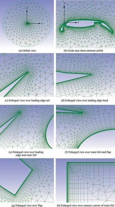
Fig. 16 Hybrid triangular grid generation over a three-element airfoil.

In the following context, the anisotropic grid quality with and without the multi-direction advancing (Section 2.4.1)and the relative advancing step factor(Section 2.4.2) are compared in Table 4. It can be seen, for Case 1, that the anisotropic grid quality coefficients of the most of initial grids(87.51%) are larger than 0.9, and after optimization, the proportion of grids whose quality coefficients are larger than 0.9 is more than 92%,while that of grids whose quality coefficient is less than 0.6 is only 0.19%.So these anisotropic grids are more suitable for viscous flow simulations. For Case 2 and Case 3,the geometries are more complicated, there are some sharp concave and convex corners, and then the anisotropic gridquality is improved more obviously than that of Case 1 since the multi-direction advancing technique and the relative advancing step factor technique help to improve the distribution of anisotropic grids during layer advancing.

Table 3 Comparison of quality between initial grid and optimized isotropic grid generated by ANN-AFM and classical AFM

Table 4 Comparison of quality between initial grid and optimized anisotropic grid generated by ANN-ALM and classical ALM

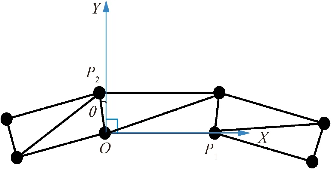
Fig.17 Evaluation of grid quality generated by layer propulsive method.

3.5. Validation of meshes

In this section, we supplied some typical results on the hybrid grids generated by the ANN-based method.We adopted three typical test cases, i.e., subsonic flow over the NACA0012 airfoil, transonic flow over the RAE2822 airfoil, and subsonic flow over the 30P30N three-element airfoil, and validated the numerical results with wind tunnel experiment data.

The freestream conditions and mesh parameters of the three cases are listed in Table 5.The growth rate of the boundary layer anisotropic quadrilateral mesh is 1.2.To simulate the boundary layer more accurately, y + of the first-layer normal grid step on the wall is about 2.

Fig.18 shows the grids generated by the ANN-based hybrid grid generation method (NACA0012 and RAE2822). For the 30P30N three-element airfoil, the grid has been shown in Fig. 16. The grid quality can be proved by the numerical results. Numerical simulations are carried out by our inhouse code HyperFLOW.The simulations are based on second-order finite volume discretization of the Reynolds Averaged Navier-Stokes (RANS) equations. Inviscid fluxes are discretized with Roe’s flux difference method and viscous interface gradients are calculated by the difference of face normal variables.Cell gradient is reconstructed by the cell-based Green-Gauss method and the Spalart-Allmaras one equation model is adopted to consider turbulence flow.

Fig. 19 depicts the lift coefficient C, the pressure coefficient Cdistributions of three cases, and experimental data.We can see that the numerical results agree well with experimental data for different cases. Fig. 20 shows the Mach number contours for three cases, which also show the reasonable flow fields and validate the ability of the present mesh generation method.

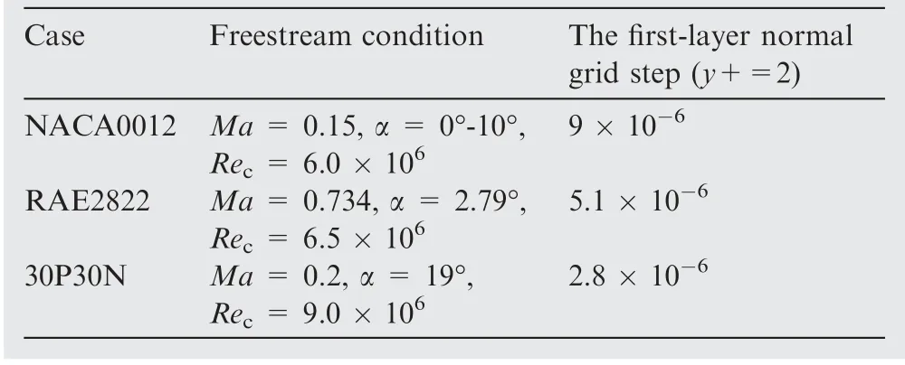
Table 5 Freestream conditions and mesh parameters of three cases

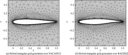
Fig. 18 Meshes of numerical validation cases.

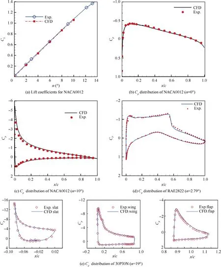
Fig. 19 Force coefficient curves and pressure coefficient distributions of airfoil cases.

Fig. 20 Mach number contours for three cases.

4. Conclusions

In this study,a novel automatic hybrid grid generation method is proposed for complex 2D geometries.Two sets of BP neural networks are established to generate the hybrid grid. The anisotropic grids are generated by ANN-based ALM,and the isotropic grids are generated by ANN-based AFM.Four kinds of grid optimization techniques are also introduced to improve the hybrid grid quality.Some typical 2D geometries are tested to validate the capability of the ANN-based hybrid grid generator. The mesh generated by the new method has shown that the ANN can predict important parameters for hybrid grid generation, and improve the adaptability of grid generation.Finally, CFD numerical simulation results and wind tunnel experimental data are compared to verify the availability of the generated mesh.

The challenge of this work is the prediction accuracy of ANNs. The ANN needs to predict its performance to avoid the generation of a new problem which it cannot solve correctly. Therefore, the focus of our study concludes the design of the structure of ANN, the input features, and the output. To improve the generalization and recognition ability of the ANN model, a new training data preprocessing method is proposed. Finally, the test results have shown that ANN can perform well in different situations.

However, this study is just an initial exploration to use the ANN to solve the hybrid grid generation. Only 2D cases are considered in this work, and it is just an improved version of the AFM and ALM essentially. Besides, the BP algorithm has some disadvantages, e.g., the slow learning rate, its tendency to converge to a local minimum, and the overfitting problem in training. So in future work, we will focus on the mechanism of grid generation and machine learning method to extend the approach to 3D complex geometries. Furthermore, more effective machine learning methods, such as deep learning and deep reinforcement learning, will be introduced into our grid generator.

The authors declare that they have no known competing financial interests or personal relationships that could have appeared to influence the work reported in this paper.

This work was supported by the National Key Re-search and Development Program of China (No. 2016YFB0200701), the National Natural Science Foundation of China (Nos.11532016 and 11672324), and the National Key Project(No. GJXM92579).