Recent progress of machine learning in flow modeling and active flow control

Yunfei Li, Juntao Chang, Chen Kong, Wen Bao

School of Energy Science and Engineering, Harbin Institute of Technology, Harbin 150001, China

KEYWORDS Data-driven modeling;Flow control;Flow field kinematics;Machine learning;Neural networks -applications

Abstract In terms of multiple temporal and spatial scales, massive data from experiments, flow field measurements, and high-fidelity numerical simulations have greatly promoted the rapid development of fluid mechanics. Machine Learning (ML) provides a wealth of analysis methods to extract potential information from a large amount of data for in-depth understanding of the underlying flow mechanism or for further applications. Furthermore, machine learning algorithms can enhance flow information and automatically perform tasks that involve active flow control and optimization. This article provides an overview of the past history, current development, and promising prospects of machine learning in the field of fluid mechanics. In addition, to facilitate understanding, this article outlines the basic principles of machine learning methods and their applications in engineering practice, turbulence models, flow field representation problems, and active flow control. In short, machine learning provides a powerful and more intelligent data processing architecture, and may greatly enrich the existing research methods and industrial applications of fluid mechanics.

1. Introduction

Accompanied by traditional fluid mechanics research, a large amount of data from experiments, flow field measurements and large-scale numerical simulations are provided.In the past few decades,benefit from the development of high-performance computing architecture and sophisticated experimental capabilities and measurement methods,big data has become a notable feature of the development of fluid mechanics.Meanwhile,corresponding methods of processing volumes of data such as database clusters proposed by Perlman et al.are used for data analysis and processing. Although efficient methods are used to process large amounts of data, these processing methods currently rely too much on professional domain expertise and complex algorithms to a certain extent.

The rapid growth of data volume is widespread in various disciplines, obtaining potential and enlightening information from data has gradually become the focus of research.In view of the upgrade of computer hardware architecture, more efficient data storage and transmission, the development of massively parallel algorithms, and the construction of open source frameworks,data-driven research methods have gained more and more attentions from industry and academia.Machine learning, especially deep neural networks, which has unique advantages when dealing with high-dimensional nonlinear problems, is rapidly integrating into the research of fluid mechanics. According to whether the data is labeled,machine learning can be roughly divided into supervised learning, semi-supervised learning and unsupervised learning.

In terms of data analysis in fluid mechanics,machine learning has gradually been applied to the fields of reduced-order modeling, reconstruction and prediction, turbulence model closure, and active flow control with many advantages. Furthermore, the fusion of machine learning and fluid mechanics will also bring challenges to corresponding algorithms, such as embedding physical prior information into models and the interpretability of research conclusions.

While the integration of machine learning and fluid mechanics is thriving, it is more worth noting that why machine learning-related algorithms are effective and under what circumstances failed.Applying machine learning to traditional fluid mechanics is a challenging research field.Researchers need to balance the pros and cons of marveling at the power of machine learning and turning specific ideas into reality. In this context, this article classifies and elaborates the application of machine learning in the field of fluid mechanics in recent years, and hopes that machine learning will further promote the development of fluid mechanics in the future.

The integration between ML and fluid mechanics has gone through a long history. In the 1950s, the perceptron proposed by Rosenblattwas designed to simulate the behavior of the human brain to find a separation hyperplane that linearly divides the training data. Researchers marveled at the classification ability of the perceptron, which has also become the basis of neural networks and later Support Vector Machines(SVM). The neural network was inspired by the research of Hubel and Wieselon the visual cortex of cats. Their experiments showed that the neural network was composed of hierarchical cells for processing visual stimuli. The excitement brought by the perceptron came to an abrupt end with the judgement of Minsky and Paperton the basic idea of machine learning: a single-layer linear perceptron could not solve the Exclusive OR(XOR)problem.The development of neural networks has stalled for the first time.

The reawakening of neural networks was accompanied by the backpropagation algorithm proposed by Hinton et al.in the 1980s, and in 1989, the Convolutional Neural Network(CNN) proposed by LeCun et al.based on the backpropagation algorithm was successfully applied to handwritten digit recognition. But these developments have not attracted the attentions of fluid mechanics researchers. In the early 1990s,Teoand Grantet al. applied neural networks to Particle Image Velocimetry (PIV) to resolve problems such as directional ambiguity.Kim et al.constructed a new adaptive controller based on neural network and used it for turbulence drag reduction. The simple control network, which employed suction and blowing on the wall based on the wall shear stress in the span direction, can reduce wall skin friction by up to 20%. However, in view of the traditional learning methods such as SVM still occupied the academic mainstream of statistical learning,the development of neural networks was still in a dormant period.

In the past ten years, with the renewed prosperity of machine learning, especially Deep Neural Networks(DNN), the integration of statistical learning methods and fluid mechanics has once again attracted the attention of many researchers. Kutzand Brenner et al.review the application of machine learning in the field of fluid mechanics in recent years. The prosperity of this integration of disciplines is largely attribute to the maturity of the deep learning architecture and the growth of computing power.The development of machine learning will largely make up for the constraints of fluid mechanics. Meanwhile, this trend will also pose a great challenge to the interpretability of machine learning.

The great success of machine learning in the fields of speech recognitionand signal processingin recent years is significantly different from its application in fluid mechanics. Considering computer vision and speech recognition, machine learning is more like a black box, but for fluid mechanics,researchers are more eager to know the physical information contained in the model and its principles. For unsteady flow,there are high-dimensional, non-linear,and large-scale temporal and spatial characteristics in fluid flow. The ability of machine learning to recognize these characteristics and why it is effective or failed remains to be explored in depth. As far as experiments are concerned,repeated experiments in fluid mechanics such as wind tunnel experiments are costly. Using numerical simulations to prepare large amounts of data will also consume a large amount of computational cost. Whether machine learning algorithms and models are equally effective in multiple experiments and various numerical simulation data remains to be resolved.

In terms of fluid dynamics control, machine learning has gradually emerged, especially interactive learning based on Reinforcement Learning (RL). Reinforcement learningis one of the paradigms and methodologies of machine learning.It is used to describe and solve the problem that agents use learning strategies to maximize returns or achieve specific goals during their interaction with the environment.In the use of RL for fluid dynamics control, the definition and design of the objective optimization function directly affects the optimization effect of the flow field and the difficulty of convergence of the model. In addition, many fluid systems are nonstationary, even for stationary systems, it also requires an expensive cost to design training algorithms to help the model achieve convergence of statistical results.

Moreover, the conclusions drawn from researches related to fluid mechanics should usually be interpretable and generalizable, and the experimental methods or numerical models obtained should have certain performance guarantees. In this regard, the integration of machine learning and fluid mechanics is facing great challenges,which in turn will surely promote the progress of machine learning algorithms.

These non-exhaustive challenges will not prevent the integration of machine learning and fluid mechanics. On the contrary, the problems encountered in the process of fusion of disciplines will inevitably promote the development of the two disciplines.

The structure of this review is as follows: Section 2 will explain the basic principles of ML, and then the research on flow field modeling with ML will be explained in the Section 3. The research on active flow control with ML will be introduced in Section 4. In the conclusion, a summary and outlook on the application of ML in fluid mechanics will be provided.

2. Fundamentals of machine learning

Machine learning is a discipline in which computers build probability statistical models based on data and use the models to predict and analyze data. Simononce gave the following definition of learning:if a system can improve its performance by performing a certain process, it is learning. The basic assumption of machine learning about data is that similar data has certain statistical regularity, which is the premise of machine learning. Machine learning is mainly composed of supervised learning, semi-supervised learning, and unsupervised learning. For supervised learning, the method can be summarized as follows: starting from a given, limited data set,assuming that the data are Independent and Identical Distributed (IID), and assume that the model to be learned belongs to a set of certain functions, called hypothesis space;apply an evaluation criterion to select an optimal model from the hypothesis space, so that the model can predict the unknown test data optimally under the given evaluation criteria.

2.1. Supervised learning

The task of supervised learning is to learn a model so that the model can make a good prediction of its corresponding output for any given input.At the same time,supervised learning is an extremely important branch of statistical learning.Each specific input is an instance, which is usually represented by a feature vector, and the space in which the feature vector is located is called the feature space. The models are actually defined in the feature space.The purpose of statistical learning is to select the optimal model from the hypothesis space. In practical applications,the loss function is usually used to measure the quality of model prediction. The loss function is usually defined as Eq. (1):

where the Structural Risk Minimization (SRM) is a strategy proposed to prevent overfitting, data input (x） and output(y)are sample pairs from a probability distribution,λJ（f）represents a regular term used to weigh empirical risk and model complexity. Regularization conforms to the principle of Occam’s razor: among all possible models, one that can explain the known data well and is very simple is the best model.

2.1.1. Neural networks

Neural network should be the most popular learning architecture in the field of machine learning in recent years. The universal approximation theorem proposed by Hornik et al.shows that if a feedforward neural network has a linear output layer and at least one hidden layer with any kind of ‘‘squeezing” activation function (such as logistic or sigmoid), it can approximate any measurable function from one finitedimensional space to another with arbitrary precision. The most classical model of the neural network in the context of pattern recognition is the feed-forward neural network, also known as the Multilayer Perceptron (MLP). Feedforward neural network is composed of multi-layer neurons, and the output of each layer serves as the input of the next layer. It is a kind of quintessential deep learning model for modeling high complexity data through multi-layer nonlinear transformation. Convolutional Neural Networks (CNN) proposed by LeCun et al.are a specialized kind of neural network for processing data that has a known, grid-like topology. Compared with fully connected operation, the biggest preponderance of convolution operation is weight sharing and sparse interaction,which also makes the parameters of the convolutional layer much smaller than that of the fully connected layer, and makes it more suitable for image recognition. The LeNet-5 CNN architecture proposed by LeCun et al., the first one successfully applied to handwritten number recognition,is shown in Fig. 1.With its powerful capabilities, CNN has now becomes the cornerstone of object detection,image super-resolution and other fields.

For CNN and feedforward neural networks, the links between neurons are limited to layers, while for Recurrent Neural Networks (RNN), neurons in each layer can also have links to each other. In the 1980s, the RNN proposed by Hopfieldcould not effectively solve the problems of gradient vanishing/explosion,which made it difficult to train the network,and its early application was limited.An epoch-making change appeared in 1997,the Long Short-Term Memory(LSTM)network proposed by Hochreiter and Schmidhubereffectively alleviated the long-term problem of RNN and gradient explosion by constructing a well-designed gate structure in the cell.Nowadays, LSTM plays an indispensable key role in speech recognition,text generationand other fields by virtue of its excellent ability to deal with time-series related problems.The structure of the standard RNN and LSTM are shown in Fig. 2.In addition to the standard LSTM structure, Gers and Schmidhuberproposed an LSTM variant with extra connections called peephole connection: the previous longterm state cis added as an input to the controllers of the forget gate and input gate.In addition,the Gated Recurrent Unit(GRU)cell proposed by Cho et al.in 2014 is a simplified version of the LSTM, and it seems to perform just as well as LSTM. In general, LSTM or GRU cells are one of the main reasons behind the success of RNNs in recent years, in particular for applications in Natural Language Processing (NLP).

It’s worth mentioning that,how to prevent gradient vanishing/exploding is the most important consideration in the process of deep neural network training. In 2015, Ioffe and Szegedyproposed a technique called Batch Normalization(BN) to address the vanishing/exploding gradients problems,and more generally the problem that the distribution of each layer’s inputs changes during training, as the parameters of the previous layers change (which they call the Internal Covariate Shift problem).In addition,techniques such as drop outand early stopping to suppress overfitting are also worthy of attention.

2.1.2. Classification: Support vector machine and decision trees

Fig. 1 Structure schematic of LeNet-5 model adopted from LeCun et al.20

Fig. 2 Structure schematic of RNN and LSTM network (figure was based on the idea from Hochreiter and Schmidhuber24).

Classification is the core problem of supervised learning.When the output variables are distributed with a finite number of discrete labels,the prediction problem turns into the classification problem.For classification problems,the two most commonly used and classic methods are SVM and logistic regression.SVM is a two-class classification model. Its basic model is a linear classifier with the largest interval defined in the feature space. The largest interval makes it different from the perceptron. Furthermore, the SVM can use kernel techniques proposed by Boser et al.,which makes it essentially becomes a nonlinear classifier. In reality, soft interval SVM proposed by Cortes and Vapnikare more suitable for training data which is approximately linearly separable.For a given training data set,the separation hyperplane learned by maximizing the interval or solving the corresponding convex quadratic programming problem is shown as Eq.(2),and the corresponding classification decision function is shown as Eq. (3).

where x represents data input, wand brepresent the weight vector and bias,respectively.Drucker et al.further extended SVM to make it suitable for regression problems. For linearly inseparable training data, learning a nonlinear support vector machine by using a kernel function is equivalent to implicitly learning a linear support vector machine in a highdimensional feature space.

Like SVMs, decision trees are versatile machine learning algorithms that can perform both classification and regression tasks, and even multioutput tasks. Decision trees are also the fundamental components of random forests,which are among the most powerful ML algorithms available today. The decision tree learning process usually includes three steps: feature selection, decision tree generation and decision tree pruning.These ideas are mainly derived from the ID3 algorithm proposed by Quinlanin 1986 and the C4.5algorithm proposed in 1992, as well as CART algorithm proposed by Breiman et al.in 1984.

2.2. Semi-supervised learning

The learner does not rely on external interaction and automatically uses unlabeled samples to improve learning performance,which is semi-supervised learning. For semi-supervised learning,two main categories will be introduced:Generative Adversarial Networks (GAN) and RL, both of which belong to the self-training paradigm.

2.2.1. Generative adversarial networks

So far, the most noticeable success of deep learning has focused on discriminative models, which map highdimensional and complex sensory inputs to low-dimensional class labels, such as SVM and conditional random fields.The generative model learns the joint probability distribution p（x，y） through input data, and then produces the posterior conditional probability distribution p（y|x）. Typical generative models include Naive Bayesian Method and Hidden Markov Model (HMM). Traditional generative methods have more difficulties in approximating many difficult probability estimation problems, such as maximum likelihood estimation,which leads to the fact that deep generative models have had less of an impact. The GAN proposed by Goodfellow et al.sidesteps these difficulties.

The application of MLP to GAN is the most straightforward application. In addition, some variants such as Deep Convolutional Generative Adversarial Networks (DCGAN)are also worthy of attentions in certain scenarios. GANs are inspired by the two-player minmax game, the model training can be performed by optimizing the value function V（G，D）which is shown as Eq. (4):

where G called generator is a differentiable function represented by a MLP with parameters θ（g） that maps random noise z to the input data space x, D called discriminator is the second MLP that outputs a scalar value to represent the probability that the input data is from the real sample data and not the results of the generator,Eand Erepresent the expectation that the data comes from the input and the noise,respectively.For the actual training of the model,the k-step optimization for discriminator and the 1-step optimization for generator are executed, which makes D always stay near its optimal solution as long as G changes slowly enough.This self-training mode of GAN has attracted a lot of interest,but its inherent training disequilibrium and mode collapse problems pose a great challenge to the convergence of training.In addition, the loss of generators and discriminators cannot indicate the progress of training. The WGAN proposed by Arjovsky et al.introduced the Wasserstein distance to the GAN, instead of the original Kullback-Liebler (KL) divergence, and greatly resolved the problem of disequilibrium of the original GAN.

In the category of generative models, in addition to the GAN already introduced, Variational Autoencoder (VAE)proposed by Kingma and Wellingand PixelRNN proposed by Oord et al.also worthy of attentions. The goals of VAE and GAN are basically the same, they both hope to build a model that generates target data x from latent variable z, but the implementation is different.

2.2.2. Reinforcement learning

RL is one of the most exciting fields of machine learning today,and also one of the oldest. In RL, a software agent makes observations and takes actions within an environment, and in return it receives rewards. Its objective is to learn to act in a way that will maximize its expected long-term rewards. In other words, the agent acts in the environment and learns by trial and error to maximize its pleasure and minimize its pain.It is this precise approximation that makes it highly suitable for dynamic control problems in fluid mechanics. The RL algorithms can be classified into policy based, a=π（s）defines the agent’s behavior α at a given time with the state s of the system, and value based, v（s） tells us the maximum expected future reward the agent will get at each state. For fluid mechanics,the algorithm based on policy gradient is obviously more suitable for complex multi-scene flow control problems.The schematic diagram of RL based on policy gradient is shown in Fig. 3.

The basic idea of RL comes from the Markov Decision Process (MDP) proposed by Bellmanin the 1950s. Early applications of RL are limited to domains where features can be made manully and have a fully observed lowdimensional state space. In 2015, Mnih et al.used the method of training deep neural networks to build a novel artificial agent,named Deep Q Network(DQN),using end-to-end deep reinforcement learning to directly learn successful strategies from high-dimensional sensory input. DQN is a typical RL algorithm based on value function,to choose which action to take given a state with the highest Q-value (maximum expected future reward will get at each state). But for some continuous action scenes, because DQN assigns a score to any possible action, it is no longer suitable in scenes with infinite possibilities of actions.The method based on policy gradient π（a|s）=P［a|s］, is more suitable for scenarios with infinite action possibilities, and it can learn stochastic policies,which means that exploration/exploitation trade off don’t need to be performed. But both of these methods have big drawbacks. That’s why, today, a new type of RL method which we can call a ‘‘hybrid method”: Actor Critic, proposed by Mnih et al.,is more popular.For actor critic,two neural networks will be used,a critic that measures how good the action taken is (value-based), and another is an actor that controls how agent behaves (policy-based). The state of the art deep RL algorithm Proximal Policy Optimization (PPO) proposed by Schulman et al.is exactly based on Actor Critic. We believe that deep RL algorithms based on PPO are more suitable for active flow control problems in fluid mechanics.

Although deep RL has made amazing achievements, it is still confronted with some intractable problems, especially for complex scenes where some specific reward functions are difficult to obtain in fluid mechanics. The reverse RL algorithm proposed by Ng and Russellis designed to find an efficient and reliable reward function.To resolve the problem that the model doesn’t have the ability to planning,that is,the ability to consider subsequent rewards,the value iterative network proposed by Tamar et al.embeds the value iterative planning algorithm through convolution into the deep neural network,making the model have stronger generalization ability than DQN.

2.3. Unsupervised learning

Unsupervised learning is a machine learning paradigm that learns the statistical laws or internal structure of data from unlabeled data. It mainly includes clustering, dimensionality reduction and probability estimation. Unsupervised learning is mainly used for data analysis or pre-processing of supervised learning.The basic idea of unsupervised learning is to perform some compression on a given matrix data, assuming that the result of compression with the smallest loss is the most essential structure.

2.3.1. Dimensionality reduction: Proper orthogonal decomposition, principal component analysis and autoencoder

Proper Orthogonal Decomposition (POD) is the most fundamental data-driven method for modal analysis of the entire unsteady flow field, which is equivalent to Principal Component Analysis(PCA).The principle of POD is that each instantaneous flow field can be represented by the linear weighted sum of orthogonal basis vectors called POD modes.However,since each instantaneous flow field is processed independently in the POD,it is difficult to understand the temporal characteristics of the flow field by the POD mode itself. PCA uses orthogonal transformation to convert the observed data represented by linearly dependent variables into a few data represented by linearly independent variables. The linearly independent variables are called principal components. The number of principal components is usually smaller than the number of original variables. In 1933, Hotellinggeneralized PCA to apply to random variables. It is worth noting that PCA can also use the kernel methodintroduced in SVM,making it possible to perform complex nonlinear projections for dimensionality reduction.

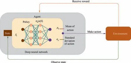
Fig. 3 Deep reinforcement learning schematic (figure was adapted from Brunton et al.42).

Researches have been carried out on the low-dimensional characteristics representation of the flow field using methods such as PCA. However, these dimensional reduction methods are linear and rely on strong assumptions. Recently, deep learning,which is a state-of-the-art non-linear mapping method, is used as a more flexible learning paradigm for low-dimensional representation of data. Autoencoders (AE)are artificial neural networks capable of reducing dimensions and learning efficient representations of the input data, called codings, without any supervision. However, the deviation between input and output is not a compelling reason that really affects the feature extraction effect of the model.Another way proposed by Vincent et al.to force the AE to learn useful features is to add noise to its inputs, training it to recover the original, noise-free inputs.

Locally Linear Embedding(LLE)proposed by Roweis and Saulis another very powerful non-linear dimensionality reduction technique. It is a Manifold Learning technique that does not rely on projections like the previous algorithms. In addition, some other dimensionality reduction methods such as Isomap and t-distributed Stochastic Neighbor Embedding(t-SNE) are also worthy of attention.

2.3.2. Clustering: k-means

Clustering is a data analysis method that combines a given sample into several categories based on the similarity or distance of their features.Intuitively,similar samples are concentrated in similar classes,and dissimilar samples are scattered in different classes. The purpose of clustering is to discover the characteristics of data through the obtained classes, and it has a wide range of applications in the fields of data mining and pattern recognition. The most commonly used clustering algorithms are hierarchical clustering and k-meansclustering. Hierarchical clustering assumes that a hierarchical structure exists between samples. k-means clustering divides the sample set into k subsets,and each sample has the smallest distance to the center of its class.

2.4. Other important topics: Transfer learning and Gaussian process

There are also some ML algorithms that are not covered in this review but are also worthy of attention from the fluid mechanics community.For the effective application of many ML algorithms,the premise is that the data used for training model and future prediction must be located in the same feature space and have the same distribution,that is,to meet the requirements of independent and identically distributed. However, this assumption may not be fully satisfied for many practical problems. For example, we are interested in the classification task in one domain, but sufficient labeled training data exist in another domain, where the data distribution of the latter may not be exactly the same as that of our target domain. In this case, transferring the knowledge domain with a large amount of labelled data to the target domain we are interested in will save a lot of effort in labelling data. In recent years,transfer learning has gradually attracted the attention of researchers and has been used to solve such problems.Transfer learning can be defined as the ability of the system to recognize and apply the knowledge and skills learned from previous tasks to new tasks.Different from multi-task learning,learning both source task and target task simultaneously, transfer learning pays more attention to target task, which also makes source and target task no longer symmetric in transfer learning.For transfer learning,an important question in most situations is‘‘when to transfer”.Relying on brute force to transfer irrelevant source domain knowledge to the target domain may be unsuccessful,that is,negative transfer.According to the different domains and tasks of the source and target, transfer learning can be divided into the following categories:inductive transfer learning, transductive transfer learning, and unsupervised transfer learning.The CNN-based transfer learning schematic is shown in Fig.4.We recommend readers to refer to the reviews on transfer learning by Panand Shaoet al.

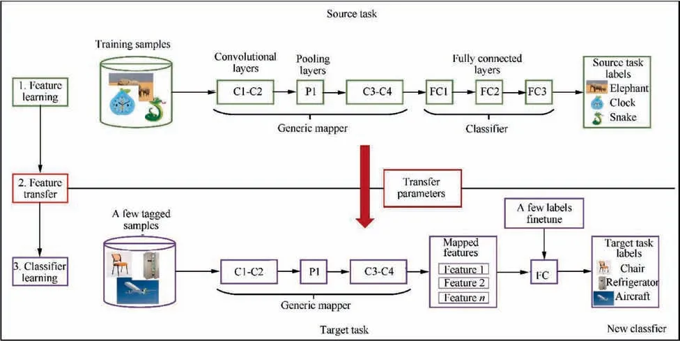
Fig. 4 Schematic of transfer learning model based on CNN.

Gaussian Process(GP)is a kind of random process in probability theory and mathematical statistics.It is an extension of multivariate Gaussian distribution and is used in ML, signal processing and other fields. The GP can be defined as: for all x=［x，x，···，x］, f（x）=［f（x），f（x），···，f（x）］ obeys the multivariate Gaussian distribution, then f is a Gaussian process, which can be expressed as Eq. (5):

where μ（x）represents the mean function and returns the mean of each dimension, κ（x，x） represents the covariance function(also called kernel function)and returns the covariance matrix between the each dimension of two vectors. A GP is uniquely defined by a mean function and a kernel function,and a finitedimensional subset of a Gaussian process obeys a multivariate Gaussian distribution. The kernel function is the core of the GP that generates a covariance matrix (correlation coefficient matrix) to measure the ‘‘distance” between any two points.The most commonly used kernel function is the Gaussian kernel function, which is also called the Radial Basis Function(RBF)kernel.GP regression naturally supports the prediction uncertainty (confidence interval) of the model, and directly outputs the probability distribution of the value of the prediction point. However, as a non-parameter model, the GP regression needs to solve inverse matrix for all data points in the process of each inferring. When the data volume is large,the GP becomes very intractable. For a more detailed introduction to the Gaussian process,please refer to Rasmussen’swork.

3. Flow modeling with machine learning

For nearly a century,the basic laws of physics such as conservation laws have deeply occupied the dominant position in the research of fluid mechanics, and have greatly promoted the research and application of fluid mechanics. However, for the flow with high Reynolds number that is common in the aerospace, using Direct Numerical Simulation (DNS) based on directly solving the Navier-Stokes equations to obtain the flow field parameters will consume huge computing resources,which is far from the degree of practical engineering application. On this basis, many turbulence models have been developed to approximate these conservation equations, or specific experiments can be performed to obtain corresponding results. However, considering that the experiment largely depends on the specific configuration,and the numerical simulation cannot control the flow in real time, the reconstruction and prediction of flow field parameters based on ML and the active flow control based on RL provide a new avenue for traditional fluid mechanics research.

For complex high-dimensional unsteady flow fields, traditional flow characteristics representation methods, such as time serialization of the pressure on the surface, cannot comprehensively clarify the spatial-temporal effects of flow.Data-driven methods such as dimensionality reduction can extract the key features and main patterns of flow that are used to describe the essential internal structure of the data.Among these data-driven methods, POD, proposed by Lumley,is one of the most notable examples. With the improvement of numerical calculation capabilities and the enrichment of experimental measurement methods, fluid mechanics is gradually becoming a research field with abundant data,which means that it is gradually applicable to ML algorithms.

The flow field feature representation and turbulence modeling based on machine learning will be elaborated in this section respectively.

3.1. Flow field representation

Pattern recognition and data mining are the core of machine learning algorithms. Due to the inherent high-dimensional nonlinearity of the flow field, it is particularly intractable to predict and analyze the spatial-temporal behavior of the flow field. We discuss the reconstruction and prediction of flow field,followed by the super-resolution and denoising.Furthermore, the extraction of flow features and the reduced-order model will also be involved.

3.1.1. Reconstruction and prediction

Nowadays, the multi-dimensional aerodynamic database for aeronautical engineering is widely used in the fields of design,optimization and control,etc.The term multidimensional refers to multiple parameters, such as altitude, Mach number, and angle of attack. The amount of data required often increases exponentially as the number of dimension increases,also known as a dimensional disaster. To reduce computational consumption, a common strategy is to find a suitable surrogate model.Commonly used surrogate models can be divided into three categories, namely multi-fidelity models, simplified models based on projection, and data fitting models. The latter, also known as data-driven models. Compared with simplified projectionbased models such as POD,data-driven models aim to establish the mapping relationship between parameters in a‘‘black box”manner.The reconstruction and prediction of flow field parameters are formally based on this concept.

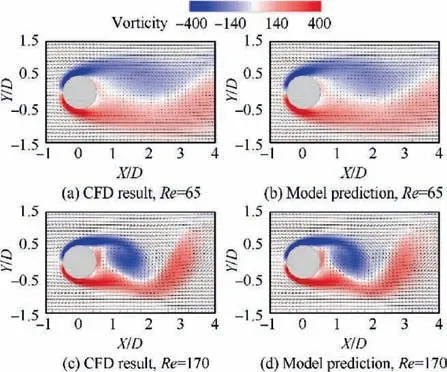
Fig. 5 Comparison of instantaneous flow field of cylinder between model prediction and CFD results.60

One interesting application of ML in fluid dynamics is to investigate the mapping relationship between fluid parameters.By data-driven methodology, a model can be regressed by establishing the intrinsic connections between these parameters. The fusion CNN constructed by Jin et al.with or without a pooling layer uses the pressure of the cylinder surface to predict the wake velocity.The comparison results of its prediction of instantaneous velocity field of the cylinder are shown in Fig. 5.This model can simultaneously capture accurate spatial-temporal information of the flow field around the cylinder,and the features that are invariant of small translations of pressure fluctuations on the cylinder surface in temporal dimension. Aiming at the unsteady flow field prediction of the flow around a cylinder, Lee and Youused GAN to extract fluid dynamics characteristics, and analyzed the impact of the proposed physical loss function on the prediction results. The physical loss function is designed to explicitly provide conservation information to the model. Compared with using generative methods to construct models, the most important enlightenment of Lee and You’s research is to remind researchers of the importance of combining prior physical conservation laws with ML models. Furthermore, Han et al.designed a novel hybrid neural network using the ConvLSTMnetwork to capture spatiotemporal dynamics mapping from high-dimensional complex flow fields without using any explicit dimensionality reduction methods, and predict the future flow field around a cylinder based on the captured features. The research of Han et al.shows that it may be more effective to combine LSTM and convolution to study the temporal effect of unsteady flow field. In addition,LSTM is also used to predict turbulent shear flowwhich aims to evaluate the feasibility of using neural networks to predict low-order representations of near-wall turbulence. In addition to predicting the turbulence characteristics, Kim and Leeused CNN to predict the local heat flux by assuming that the local heat flux in the normal direction of the wall could be explicitly expressed through the multi-layer nonlinear neural network according to the shear stress and wall pressure fluctuation of the nearby wall. In addition to comparing the Root-Mean-Square Error (RMSE) and correlation coefficient between the model prediction results and DNS, the statistical properties such as Probability Density Function (PDF) and high order moment are also analyzed and compared. Raissi et al.used a coupled neural network with discrete spatialtemporal data as input to solve the velocity field and pressure field around the cylinder and the motion of the structure,instead of using the numerical discrete method to solve the fluid mechanics equation and the dynamic equation of the structure motion. Given some limited and scattered information about the velocity field, the lift and drag on the surface of the cylinder are predicted. As a part of the loss function,the governing equation plays the role of regularization.

Combining these studies, it can be found that embedding necessary flow field information such as flow control equations and conservation laws into the neural network model can deepen the interpretability and generalization ability of the ML model. In addition, the specific skills of building models also need to consider specific problem scenarios, such as whether to use LSTM networks related to time series when reconstructing unsteady flow fields. More importantly, in the analysis of results, statistical analysis of turbulence characteristics is essential, such as turbulence energy spectrum.

In the field of aeronautical engineering, obtaining the flow field around the airfoil is an important factor for obtaining pressure and skin friction, as well as for studying flow separation, transition, wake vortex, etc. These parameters and flow characteristics are very important for the design of aircraft wings and helicopter rotor blades. Traditionally, the flow field around an airfoil is obtained by solving the Navier-Stokes equation on a computational grid with appropriate boundary conditions. However, when optimizing the airfoil and solving the fluid-structure interaction, the CFD calculation is still relatively time-consuming,which requires a lot of iterative calculations. The emergence of efficient deep learning tools has brought a new modeling paradigm to physical systems. By deploying machine learning technology, existing scientific databases can be used for aerodynamic modeling, analysis and design.

The use of ML to predict the flow field around the airfoil has also made gratifying progress. The flow field around the airfoil is considered as a function of its geometry, angle of attack and incoming flow Reynolds number.Sekar et al.used CNN to extract the geometric features of the airfoil and input them into the MLP together with the Reynolds number and the angle of attack to predict the flow field around the airfoil.Based on the same idea, Zhangand Yilmazet al. used CNN to predict the lift coefficient of the airfoil, and the CNN-based model has smaller geometric constraints in terms of prediction accuracy. Hocˇevar et al.utilized Radial Basis Function Neural Network(RBFNN)to estimate the turbulent wake.Based on the same idea,Bhatnagar et al.constructed a ML framework based on CNN to predict the flow field of different airfoils under variable flow conditions, making it possible to study the effects of airfoil shape and flow conditions on aerodynamic parameters in real time.Combining these studies,it can be found that the prediction of the flow field around the airfoil is usually achieved by constructing the mapping relationship between the geometric parameters of the airfoil and the surrounding flow field parameters. In essence, the use of deep neural networks to build models is more like a modeling method that accurately implements interpolation, and its ability to extrapolate and generalize remains to be verified.

In addition,drogue detection is a basic problem in the close docking stage of autonomous aerial refueling. Wang et al.used CNN to achieve highly robust drogue detection,avoiding the traditional method that requires artificial features to be placed on the drogue. The experimental results show that the method based on deep neural network is more excellent in accuracy, detection speed and robustness than traditional methods.Besides,the reliability of the Engine Electronic Controller (EEC) is an important issue affecting the safety of aircraft engines, and it is of great significance to accurately evaluate its reliability.Wang et al.used Bayesian deep learning to propose a reliability assessment method for the Mean Time Between Failures (MTBF) in the design phase considering complex products and uncertain task profiles.This reliability assessment method can accurately evaluate the MTBF of the EEC without referring to physical experiments.

For the transonic or supersonic cascades of aero-engine compressors,the high back pressure generated by the combustion chamber causes the shock wave structure in the cascade channel to be gradually pushed toward the cascade lip, which will cause a stall in severe cases.As a result,the intake capture flow rate of the cascade drops sharply.Therefore,for the compressor cascade of an aero engine, accurate, efficient and prompt airflow status monitoring is indispensable.Traditional state monitoring methods mainly include gas path analysis,installing miniature accelerometers on rotor blades,and collecting vibration data of blade cascades.However, due to their inherent limitations, these methods are difficult to intuitively and comprehensively reflect the state of the flow field.More efficient methods for monitoring the flow field conditions are urgently needed.The traditional method of obtaining flow field structure based on schlieren is shown as Fig.6.The flow field reconstruction method based on deep learning can reconstruct a more comprehensive flow field based on less local information, which provides a new way to develop a prompt and efficient flow field state monitoring method.

In terms of flow field reconstruction, Li et al.used transposed convolution network as shown in Fig. 7and residual network to reconstruct the flow field of supersonic cascade SAV21 under the condition of fixed incoming Mach number and continuous change of back pressure,and obtained the flow field image of cascade channel by using discrete pressure value of cascade wall surface.The reconstruction relative error in the test set was less than 3.5%. In addition to using experimental data,Li et al.explored the ability of deep neural networks to identify the shock wave structure of the flow field under the complex and variable working conditions of variable incoming Mach number and back pressure based on numerical simulation data. In terms of the isolator of scramjet engine, Kong et al.used the CNN of the fusion path to achieve highprecision flow field reconstruction, and the detection accuracy of the leading edge of the shock train was more robust than traditional methods.The comparison results of the shock train leading edge location detection between CNN-based model and traditional methods are shown in Fig. 8.In essence,Liand Kongconstructed the mapping relationship between wall pressure information and flow field structure,but only considered the change of flow field structure during the rise of back pressure, and did not further explore whether there was hysteresis in the decline of back pressure.

In addition to the state monitoring of the flow field, the fault diagnosis of rotating machinery is also of great significance in the industry.Recently,fault diagnosis methods based on ML have become a research hotspot. In this respect, Li et al.proposed a CNN-based infrared thermal imaging fault diagnosis method. According to the bearing data, Zhang et al.converted the original signal into a two-dimensional image, and used CNN to extract and classify fault features,which effectively improved the accuracy of bearing fault diagnosis. Considering that the acquisition cost of fault samples is relatively expensive and inevitably contains noise, the identification performance of the diagnosis model is not ideal. The weighted extension neural network constructed by Wang et al.built a corresponding fault diagnosis model for small samples turbo-generator sets with noise through different types of connection weights and improved correlation functions.

In general,in terms of flow field reconstruction and prediction, most of the existing researches use convolutional neural networks. In addition, considering the unsteadiness of flows,some researches combine LSTM with convolution to reveal the unsteady spatial-temporal effects of flow and have made some preliminary progress. In principle, using ML to reconstruct and predict flow fields may be a technical challenge but is ordinary in physical principles. The latest developments in ML-based methods are mathematically based on function approximation, which is also common in fluid research. The difference is that the previous fluid research based on function approximation mainly combines dimensional analysis and physical laws, and the mathematical form is explicit, with few input and output.In contrast,with ML-based approaches,the requirements for functions can be more freely specified and tailored to specific problems than ever before.

It is worth noting that deep learning often means that the amount of effective data that used for model training far exceeds the number of parameters of the model, which will lead to the occurrence of overfitting and the poor extrapolation ability of the model, making it impossible to accurately predict the unknown situations. Deep learning once again attracted the attention of the public is the excellent performance of the CNN on the ImageNetdata set in 2012, but the training data set for problems such as image classification or speech recognition is very large, making the prediction of unknown data very likely falls within the range of interpolation in the data set. In other words, the predictive ability of the model depends on the data used for training, that is, the model can only learn the intrinsic features embedded in the data. Although fluid mechanics is gradually becoming a data-rich subject by virtue of numerical simulation and increasingly abundant experimental measurement methods, it is still very different from the application mode of image classification.We believe that the establishment of a large enough,labeled fluid database for a certain scenario will further promote the deployment of machine learning-based algorithms.

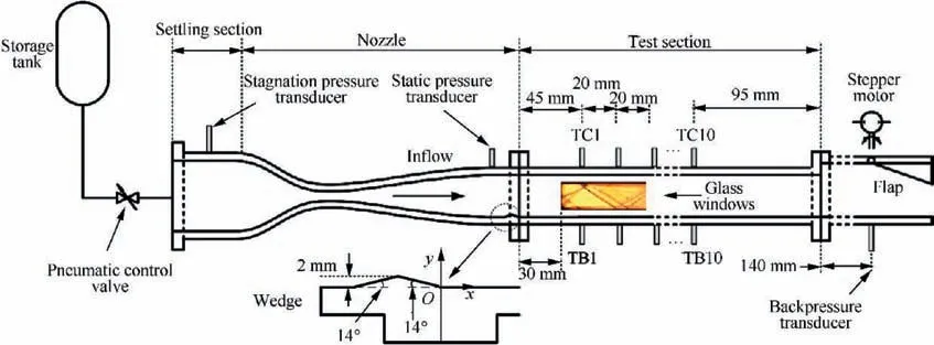
Fig. 6 Schematic of scramjet isolator model installed in direct connected wind tunnel used for monitoring airflow state.77

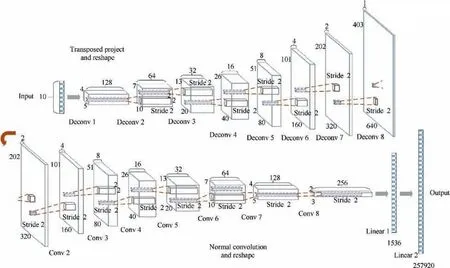
Fig. 7 Architecture of transposed convolutional network proposed by Li et al.78 (‘‘Deconv” denotes transposed convolution; ‘‘Conv”denotes convolutional operation; and ‘‘Linear” denotes fully connected layer).

3.1.2. Super-resolution and denoising

For the practical application of aeronautical engineering,obtaining the complex structure of the turbulent flow field,whether it is numerical simulation or experimental fluid mechanics, has always been a long-term challenge. In CFD,complex details of turbulent structures can be obtained using DNS with billions of grids, but this requires costly computing resources. For experimental fluid mechanics, PIV or schlieren can be used to capture major large structures well,but the spatial resolution is limited by the inherent characteristics of the camera and external devices. Considering that it is difficult to obtain fine-scale structures in turbulent flow in many cases of practical engineering, it is essential to enhance the spatial resolution of the flow field. Recent developments in superresolution technologies based on deep learning algorithms for estimating high-resolution images from low-resolution images using Artificial Intelligence (AI) have received increasing attentions.

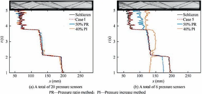
Fig. 8 Comparison of detection results of leading edge of shock train between CNN and traditional methods with different configuration of pressure sensors.77

Super-Resolution (SR) refers to the process of reconstructing the corresponding high-resolution image from the observed low-resolution image.Super-resolution belongs to the category of inverse problems.For a low-resolution image,there may be multiple different high-resolution images corresponding to it,subsequently, prior information is usually added to normalize the solution of high-resolution. In traditional methods, the prior information could be learned through several examples of low-high resolution images that appear in pairs. The SR based on deep learning directly learns the end-to-end mapping function from low resolution images to high-resolution images through neural networks.

Recently, Dong et al.proposed the Super-Resolution Convolutional Neural Network (SRCNN) with only three convolutional layers to solve the problem of image superresolution. Compared with traditional interpolation and sparse coding methods, the accuracy of image reconstruction was greatly improved. In addition, a highly accurate SR method based on a Very Deep Convolutional Network(VDSR)proposed by Kim et al.by combining the CNN with the residual structurefurther improves the accuracy of image super-resolution. Recently, the hybrid Downsampled Skip-Connection/Multi-Scale (DSC/MS) model proposed by Fukami et al.carried out the research of turbulence superresolution for two-dimensional cylinder wakes,and the results showed that the model could reconstruct very accurate turbulence structures from extremely coarse turbulence images,which holding great potential in revealing the physics of complex turbulence sub-grid scale. In addition, the turbulent energy spectrum can be reconstructed accurately.More importantly, research by Fukami et al.indicates that traditional super-resolution methods based on filter operation have lowpass characteristics and may not be suitable for highfrequency problems such as turbulence. The super-resolution workflow of the turbulent flow field structure is shown in Fig. 9.The Multiple Temporal Paths CNN model (MTPC)proposed by Liu et al.takes the time series of the turbulent velocity field as input, covers both temporal and spatial information,and three temporal paths are designed to fully capture the characteristics in different time ranges.The results indicate that the model captures the turbulent characteristics such as the kinetic energy spectrum very well. The research of Liuand Jinet al. further pointed out that carefully designing multiple paths with different operations in the model may be crucial to capture the flow characteristics of different spatialtemporal scales.In addition to supervised learning,some other studies have been proposed by Xie et al.as shown in Fig.10 and Deng et al.respectively to conduct turbulence superresolution by virtue of GANs. The research of Xie et al.applied conditional GAN to the four-dimensional data set for the first time.More importantly,it proved that it is possible to train a generator with temporal coherence through the time discriminator.Large-Eddy Simulations(LES)may also benefit from the super-resolution by leveraging high-resolution data on a smaller domain to enhance the resolution on a larger imaging system.

In general, the end-to-end super-resolution method based on deep neural networks has higher reconstruction accuracy than traditional interpolation-based methods, and the data input format is more arbitrary. In the selection of specific machine learning methods, based on the existing research results, supervised learning does not perform better than generating antagonistic models. At the same time,it is also necessary to take into account the multi-scale spatial-temporal effects between input data to design a detailed model structure.

PIV is an important non-intrusive quantitative velocity measurement technique,which obtains motion vectors by analyzing continuous particle image records. This is a crucial problem that has both large input space(different particle size,concentration,and image noise)and large output space(different potential flow regimes,velocity ranges,and sub-pixel accuracy estimates). The great success of ML, especially deep learning in the image field, has provided researchers with a lot of inspiration to use deep neural networks to perform PIV speed estimation.For experimental fluid mechanics,much effort is devoted to improving the spatial resolution of PIV data. Cai et al.used CNN to extract velocity vector fields from PIV images, which allows to improve the computational efficiency without reducing the accuracy.To better extract PIV velocity from the particle images, the PIV-DCNN model proposed by Lee et al.with four level regression deep CNN was developed. In addition to using ML techniques to reconstruct the velocity field from PIV images, it can also be used to remove spurious values in the velocity field.Another way to remove spurious values is to train an autoencoder to learn useful features by adding noise to its inputs and to recover the original, noise-free inputs. The success of the ML-based model on a large number of synthetic and experimental particle images means that it paves a whole new way for accurate PIV analysis using supervised deep learning models.Especially the method based on ML can more accurately extract the fine structure of complex flow field, which greatly improves the spatial resolution of PIV. Further efforts are needed in terms of robustness and computational efficiency.

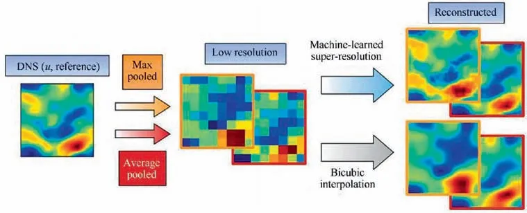
Fig. 9 Schematic of super-resolution reconstruction of turbulent velocity field.87

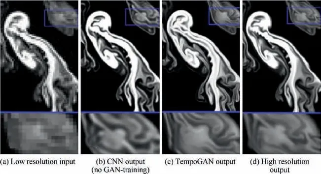
Fig. 10 Fluid flow with different resolutions.89

3.1.3. Flow feature extraction

Pattern recognition and data mining are the core applications of ML. Even in a simple aerodynamic configuration, fluid motion will exhibit complex spatial and temporal characteristics. Before the analysis of complex flows, the extraction and analysis of the dominant factors or modes of flow has become a recognized research premise. The process of extracting the features of the dominant factor of the flow field usually means the modal decomposition of the flow field. The modal decomposition of the flow field can be roughly divided into two categories, data-driven methods such as POD and Dynamic Mode Decomposition (DMD), and operator-driven methods such as Koopman analysis.The former is mainly based on flow field data, such as CFD calculation results or experimental measurements, while the latter is based on the linearized Navier-Stokes equation. Among these modal decomposition methods of flow fields, the most representative one is POD,which defines an orthogonal linear transformation from physical coordinates into a modal basis. POD was first introduced by Lumleyas a mathematical technique to extract coherent structures from turbulent flow fields. Subsequently, Sirovichproposed the snapshot method in order to solve the problem that the covariance matrix cannot be effectively solved in the actual fluid mechanics applications. Due to the significant reduction in the consumption of computing resources and the occupation of memory,the snapshot method has now been widely used in fluid data to determine the POD mode in fluid mechanics. For a more detailed overview of the modal decomposition of flow fields we refer readers to the review articles by Tairaand Berkoozet al.

DMD is another major flow field mode decomposition method, which decomposes time-resolved data into different modes,with each mode having a separate oscillation frequency characteristic. Compared with POD, DMD does not require any prior physical knowledge about the flow field.It is a purely data-driven analysis method. It is difficult to rank the decomposed modes to determine which mode is more physically important. Moreover,for POD, since each instantaneous flow field is dealt with separately in POD method,which is difficult to exploit the temporal effects of unsteady flow field. Most importantly,considering that these flow field modal decomposition methods are linear and based on strong physical assumptions,the types of flow that can be analyzed are limited.For the transonic buffeting problem of NACA0012 airfoil,Kou et al.can accurately identify the dominant flow modes by combining the High-Order Dynamic Mode Decomposition(HODMD) with mode selection criteria, which will be helpful to develop a more concise Reduced-Order Model (ROM)structure. More detailed introduction about DMD we refer readers to the article by Schmid.

Autoencoder (AE), which is a state-of-art non-linear mapping method,is utilized as a more feasible way to express lowdimensional representations. Omata and Shirayamaproposed a low-dimensional representation method of the temporal behavior of the flow field based on deep AE to visualize the temporal and spatial structure of the unsteady flow field of an airfoil. And the temporal behavior of the spatial structure of the flow field can be visualized as a trajectory in the feature space.The trajectories of the spatial-temporal structure of airfoil flow fields obtained by different methods are shown in Fig. 11.In general, the study by Omata and Shirayamaexplained the difficulties in processing time series data of unsteady flow fields, and proposed a method to visualize and compare the spatiotemporal structure of unsteady flow fields.The method consists of two stages,namely mapping the spatial structure of the instantaneous flow field to a low-dimensional feature space and displaying the mapped data in the form of time series. It should be noted that the physical meaning of axes in low-dimensional eigenspaces is not explained in detail by Omata and Shirayama.

The important significance of flow feature extraction is that the core goal of flow research is to discover the mechanism,restore a flow process to its essence, recognize the dominant mechanism in the Navier-Stokes equation, and understand the terms in the equation that control the process. The MLbased method, especially the deep autoencoder, can provide richer and more intuitive explanations in terms of dimensionality reduction and feature extraction compared with the previous POD. Therefore, compared to the way in which supervised learning builds the relationship between model parameters,deep autoencoders based on unsupervised learning may be more effective in revealing deep-level mechanisms in fluid research.

3.2. Turbulence modeling

Turbulence is a common physical characteristic in fluid flow.A sufficient understanding of boundary layer turbulence on airfoils is very important for its performance. In the combustion chamber, intense turbulence increases the mixing of fuel and air, improves overall combustion efficiency and reduces emissions. For airfoil design, fuel consumption can be reduced by delaying the generation of boundary layer turbulence over the wing surface. The representation of turbulent motion is very challenging because it involves a wide range of spatialtemporal scale effects and has a strong chaotic character.The introduction of machine learning strategies provides a new research perspective for turbulence modeling.

3.2.1. Neural network modeling

In the past few decades, neural networks have been used to model fluid systems,among which one of the most widely used is to solve differential equations using neural networks. Based on the universal approximation theoremof neural networks,Dissanayake and Phan-Thientransformed the numerical problem of solving Partial Differential Equations (PDE) into the problem of solving unconstrained minimum values.Lagaris et al.proposed to incorporate the feedforward fully connected neural network with adjustable weights into the differential equation solution to solve the initial value and boundary value problems. In the following years, the research of using neural network to solve differential equations gradually fell into a trough. With the prosperity of deep learning, this field showed vitality again. A natural analogy between differential equations and RL maybe exists faintly. E et al.proposed a new algorithm for solving parabolic partial differential equations and Backward Stochastic Differential Equations (BSDE), which is based on the analogy between BSDE and RL. Moreover, the gradient of the solution acts as the policy function, and the loss function is given by the error between the prescribed terminal conditions and the BSDE solution. Wei et al.proposed a rule-based general self-learning method based on deep reinforcement learning to solve nonlinear Ordinary Differential Equations (ODE) and PDE which is shown as Fig. 12,and embed the equations as critics into the network, which is reasonable from the physics perspective. It is worth noting that the research of Wei et al.pointed out that discrete-time solutions can be treated as multi-tasks with the same control equation.Considering the solutions are temporally continuous,the current parameters of the network provide a good initialization for the next time step, which makes the model possesses the characteristics of transfer learning. The feasibility of this method is verified by using Deep Reinforcement Learning (DRL) to solve twodimensional steady state Couette flow, which is shown as Fig. 13.

Fig. 11 Proposed visualization of spatial-temporal structure of airfoil’s flow field as a trajectory.99

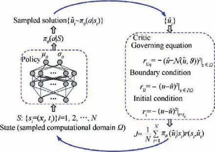
Fig. 12 DRL schematic for solving differential equations(actions are defined as candidate solutions of differential equations and are sampled from output policies of policy network,states are defined as sampling points of continuous solution domain of differential equations and are input of policy network).103

In addition, Raissi and Karniaintroduced the hidden physical model that can use the underlying physics laws expressed by time-dependent and nonlinear PDEs to extract the patterns from the high-dimensional data generated from the experiment. We also noticed that the physical-informed neural networkwhich is capable of encoding underlying physical laws that govern the data set and can be described by PDEs. The research by Raissi and Karniadakisreminds us of the possibility of using ML-based models to reveal latent variables and reduce the number of parametric studies. Furthermore, it pointed out that embedding physical information in the model when studying complex physical systems is crucial for effectively extracting information in scenarios with scarce data.

The use of neural networks to enhance or improve turbulence models is another hot topic in neural network modeling.For high Reynolds number flows around airfoils,Zhu et al.used RBF neural network to build separately models for different regions respectively, and directly constructed the mapping relationship between the turbulent eddy viscosity and the mean flow variables instead of the original PDEs. Moreover,the partition modeling strategy proposed by Zhu et al.can customize the features and model parameters of different regions, which allows the model to more accurately capture the flow characteristics of different regions. Furthermore, the Latin Hypercube Sampling (LHS) method used by Zhu et al.when constructing training samples also provides a basis for the construction of the database. The comparison of the time required for flow field calculation between the turbulence model and ML-based model is shown in Table 1.In addition,Yang and Xiaoused Random Forest(RF) and neural network to improve the four equations k-ω-γ-Aturbulence transition model by building the mapping relationship between mean flow variables and correction terms, and found that pressure gradient of streamwise played an important role in the physical information and interpretability of the model by analyzing the relative importance of each feature in the RF model. In terms of using field inversion and ML to enhance the prediction ability of turbulence model, Singh et al.proposed to infer the spatial distribution of model discrepancies through inverse modeling, and to reconstruct discrepancy information from a large amount the inverse problems into corrective model forms through ML.The research of Singh et al.showed that when the model forms are reconstructed by neural networks and embedded in the standard solver, the data-driven Spalart-Allmaras (SA) model can provide more accurate prediction of lift coefficients and stall onset angles. The comparison between the predicted results of the improved SA model and the original model on the surface pressure coefficients of airfoils at different angles of attack is shown as Fig. 14.

In fluid mechanics, Milano and Koumoutsakosused neural network to reconstruct the near-wall flow field in turbulent channel flow generated by DNS,and compared the reconstructed results with POD, indicating that this method provided improved reconstruction and prediction capability.For viscoplastic fluids, Muravleva et al.proposed the use of ML to construct a reduced-order model of Bingham medium duct flow.In terms of using neural networks to find turbulence models, Gamahara and Hattoriused neural networks to find new subgrid models of the Subgrid-Scale(SGS)stress in LES. Considering the pressure fluctuations on the airfoil surface, aerodynamic disturbances will leave certain characteristics in the pressure exerted on the airfoil surface. To what extent can the characteristics of these disturbances be resolved directly from the measured pressure,and the aerodynamic disturbances on the airfoil surface based on ML have also made preliminary progress. In this respect, Hou et al.used machine learning algorithms to investigate the extent to which the characteristics of these disturbances can be parsed from surface pressure measurements. Two different ML architectures were constructed, and the results showed that the ML model integrated with the dynamic system architecture had higher recognition accuracy. It is worth mentioning that overfitting can be reduced by injecting random noise into the input pressure data in these two methods. For porous media flow,Wang et al.constructed a neural network simplification method for multi-scale problems by constructing a dimensionality reduction space and considering multi-continuum information, which does not need to be solved like POD.

The generalization ability of ML in fluid mechanics,that is,the ability of extrapolation, has attracted much attention in practical applications. The neural network’s prediction of unknown data is more inclined to the data falling within the probability distribution range of training data,that is,the data satisfying the interpolation attribute. Thus, the selection of neural network models should be cautious.Common methods of model selection include regularization, which has been introduced before, and cross validation. Although fluid mechanics has gradually become a data-rich subject, there are still few valid data and the cost of obtaining it is still very expensive. For contexts where training data is scarce, commonly used cross-validation methods include S-fold crossvalidation and leave-one-out cross-validation.

Fig. 13 DRL to solve differential equation of steady-state Couette flow.103

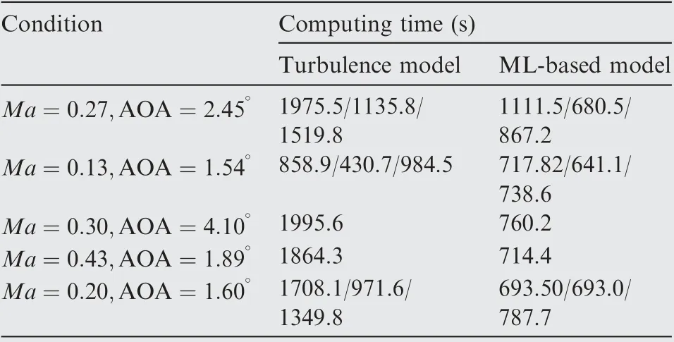
Table 1 Comparison of calculation time of turbulence model and ML-based model for flow field around airfoil.106

3.2.2. Turbulence model closure

Reynolds-Averaged Navier-Stokes(RANS)models are widely used in aeronautical engineering because of their tractable computational abilities.Most two-equation RANS models rely on the Linear Eddy Viscosity Model (LEVM) to achieve the Reynolds stress closure, which assumes a linear relationship between the Reynolds stress and the mean strain rate. However,these models cannot provide satisfactory prediction accuracy in many flows related to aeronautical engineering,such as curved flow,collision flow,and separation flow.Even if a more advanced nonlinear eddy viscosity model is proposed, it has not been widely used in aeronautical engineering due to its inability to provide sustained high performance and difficulty in convergence. Recently, there has been increasing interest in applying ML methods to provide improved Reynolds stress closure to improve the predictive ability of RANS models.

For turbulence modeling, the use of ML to study turbulence model closure is a very active field. Most recent datadriven research is evaluating the uncertainty of the RANS model. It is generally believed that the RANS model is much easier and efficient to implement in engineering than the DNS model and the LES model. The RANS model relies on the Boussinesq hypothesis, which, however, is inconsistent with the underlying physical laws of many common flows,resulting in inaccurate predictions. Therefore, it is indispensable to evaluate the uncertainty of the RANS calculation results. Ling and Templetonused three different ML algorithms: SVM, Adaboost decision trees, and RF to evaluate the uncertainty of the RANS calculation results under different configurations of based on different RANS eddy viscosity assumptions. And markers were also developed to indicate when underlying assumptions of RANS model break down.In addition, Tracey et al.investigated the uncertainties of RANS models for flame combustion in turbulent mixed layers and turbulent anisotropy in non-equilibrium boundary layer flows, respectively. In addition to using the introduced artificial neural network to calculate and express the uncertainty of the RANS model,Edeling et al.used the Bayesian model to express the uncertainty of the total solution with the probability box (p-box) to express the parameter variability across flows.In addition,the data-driven framework proposed by Geneva and Zabarasusing Bayesian deep neural networks can not only improve the predicted results of RANS,but also provide probability boundaries for fluid quantities such as pressure and velocity. The prediction results of the improved RANS model and the original model for the backward step flow are compared with the results of LES model,as shown in Fig. 15.The uncertainty of the turbulence model includes not only the uncertainty of the model form,but also the cognitive uncertainty caused by the limited training data. Using ML to quantify the uncertainty of the RANS model and improve its predictive ability has far-reaching research potential.

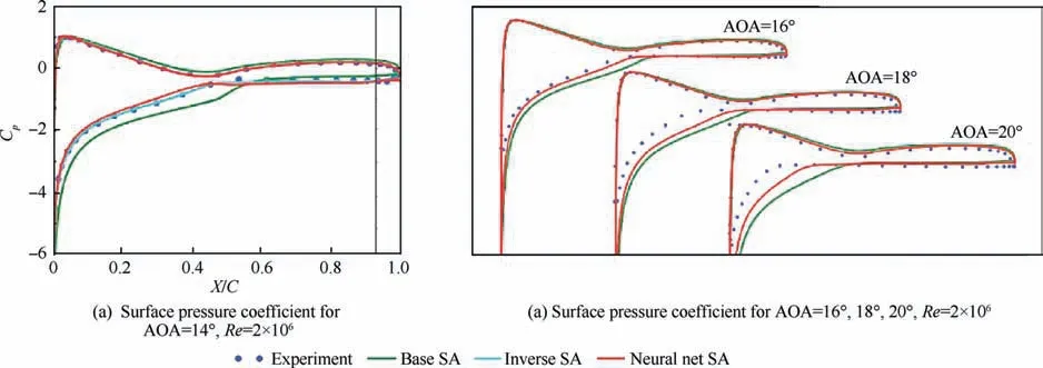
Fig. 14 Comparison of pressure coefficient between results of base SA model and ML-augmented SA model for S809 airfoil.108

In general,the use of ML to evaluate the uncertainty of the RANS model usually refers to the use of supervised learning methods to indicate areas where the RANS model has higher uncertainty due to specific model assumptions. Supervised learning compares RANS results with high-fidelity results in different flow configurations, and acts as a binary classifier to mark areas with poor RANS model accuracy. The key to this work is how to develop features, error metrics, and verification procedures to ensure that the tag classification algorithm is extended to new flow configurations.

Modeling the parameters of the turbulence model is also one of the research directions.The extreme separation of temporal and spatial scales in turbulence makes it extremely costly to resolve all scales in numerical simulations. The usual approach is to truncate these small scales and use a closure model to simulate their impacts on large scales. Commonly used methods usually include RANS model and LES model.However, these models may require careful tuning to fully match the data from numerical simulations and experiments.Tracey et al.modeled the source term of the SA model which is a one-equation closure to the RANS equations that models the transport of turbulent kinetic energy. In addition,some researches on modeling the SGS stress in LES are also worthy of attention. The uniform neural network model proposed by Wang et al.provided closure for all the components of SGS stress and considered the symmetry of SGS stress at the same time, and verified the proposed model through isotropic LES turbulence. Moreover, the research of Wang et al.found that in addition to the gradient of the filtered velocity vector, the SGS stress is also related to the second derivative of the filtered velocity vector. More importantly, they found that different SGS stress components have different dependencies on the input features,but there are certain rules.Maulik et al.used convolution and deconvolution to obtain the closure terms of two-dimensional Kraichnan turbulence to account for SGS turbulence effects.Accordingly,Maulik et al.explored the use of ML to dynamically infer the applicable areas of specific turbulence model hypotheses,so as to improve the prediction ability of turbulence dynamics for a wide range of problems. It is worth highlighting that the landmark research in turbulence modeling comes from Ling et al.,this study pointed out that embedding Galilean invariance properties into machine learning models is critical to achieving high performance and the structure of its model is shown as Fig. 16.. The Tensor Basis Neural Network(TBNN) model can not only predict anisotropic eigenvalues,but also predict anisotropic tensors while maintaining Galileo invariance. Research by Ling et al. proved that deep neural networks can provide improved Reynolds stress closure. This reminds us the importance of embedding known physical knowledge or laws into ML frameworks,which we believe will become more and more important in future during the integration of ML and fluid mechanics.For more detailed data-driven turbulence modeling, please refer to the excellent review provided by Duraisamy et al.and Durbin.

In general, the research on the closure of turbulence model combined with ML can be divided into two categories: quantitative determination of the uncertainty of RANS model and modeling of Reynolds stress in RANS model and SGS stress in LES model. Most of the ML algorithms used are based on supervised learning, and semi-supervised learning algorithms such as generative adversarial models may not be suitable for these scenarios.

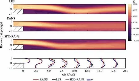
Fig. 15 Normalized stream-wise mean velocity (U-) contours of backward step flow with Reynolds number of 500 (top is LES highfidelity solution,middle is baseline RANS low-fidelity solution followed by data-driven ML augmented RANS solution, lastly is streamwise mean velocity profiles for all simulations at different cross-sections).118

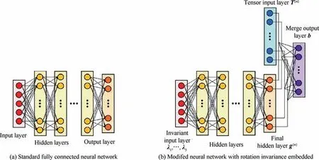
Fig. 16 Schematic of neural network architecture proposed by Ling et al.123 (b —Normalized Reynolds stress anisotropy tensor; T（n）—Isotropic tensor basic; λ1，λ2，···，λ5 —Five invariant tensors; g（n） —Scalar coefficients weighting the basic tensors).

A growing number of studies indicate that it is becoming increasingly indispensable to explicitly incorporate parts of physical information such as symmetry,constraints,or conservation laws into ML architectures.This is of great significance for promoting the interpretability of data-driven ML algorithms. The combination of ML and the closure of turbulence models presents some unique challenges and opportunities.The interpretability and generalizability of the model are the cornerstones of the research. A well-designed model will provide reasonable assumptions and judgments for previously unobserved flow phenomena. It is also important to recognize that the components of neural networks are not far away from the well-known toolbox of linear modeling. For CNNs, the convolution operation is essentially a filtering operation. The parameters of the convolution kernel are not determined by some physical laws or intuitions, but are determined during the model training process. Furthermore, the linear filtering operation in CNN usually uses key nonlinear techniques to enhance the nonlinear expression ability of the model, such as local pooling and activation functions. Therefore, we have not completely lost the interpretability of the ML model.What really needs to be explained is the measures taken to improve the approximate accuracy of the model.

3.3. Challenges for flow modeling

In spite of recent successes, several challenges remain. For data-driven flow dynamics models,the most important characteristics are interpretability and generalization ability.In addition, the physical characteristics of unsteady flow, such as multi-scale, latent variables, sensitivity to noise and disturbance, etc., need to be carefully considered when constructing a ML-based architecture.In addition,blindly using ML-based technology to use available data to predict the physical quantities of interest should be avoided, which will not help reveal the impact of latent variables and supplement the shortages of traditional analysis methods.In general,flow modeling based on ML can be divided into two major tasks:discovering unknown flow physical knowledge and improving turbulence models by integrating known physical knowledge. When considering the selection of specific models,whether it is for supervised learning or generative adversarial models, known physical constraints or conservation laws should be incorporated into the model. This is the key to the further development of fusing ML and turbulence modeling. The content and research methods of several main aspects of flow modeling carried out by ML are summarized in Table 2.

It is also worth mentioning how to achieve the correct balance between the data and model. The existing flow modeling methods focus on rediscovering known flow control equations or reconstructing known solutions.Although the closure form of the existing turbulence model is extracted as a dynamic system, the use of data-driven methods to discover unknown equations or reveal latent variables is still a problem worthy of further exploration.

Although fluid mechanics is not usually raised as a classification problem, it is actually possible. For example, you can classify the flow state under different conditions (whether it is turbulent, whether flow separation occurs, whether it is stable), so a classifier based on ML can be trained to make a judgment. However, some major hidden dangers that need to be avoided. First and foremost, the primary goal of fluid mechanics is to discover new mechanisms and restore a certain flow process to its essence.It is necessary to recognize the dominant mechanism in the Navier-Stokes equation,but many ML technologies give up on the mechanism. It relies on a datadriven approach supported by powerful computing power.The difference between the two is that instead of relying on some basic laws of physics or the filtering core pre-defined by intuition, it is better to learn from the training process.Moreover, unsteady flow requires algorithms that can solve nonlinear and multiple spatiotemporal scales, while popularML algorithms may not have such scales, and fluid-related experiments may be difficult to repeat or automate, and numerical simulation may require a very long iterative process.

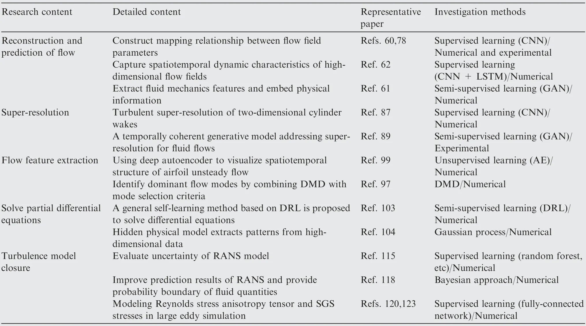
Table 2 Summary of flow modeling based on machine learning.

4. Active flow control with machine learning

Optimization and control are closely related,and with the continuous improvement of computing power, the boundary between the two becomes more and more blurred. In recent years,artificial neural networks and deep learning have become more and more popular in multiple subject areas.While it will take a long time to grasp the potential and limitations of these interdisciplinary approaches,there is growing evidence that they have amazing potential to help solve problems for which the best solutions are not yet known in theory.Especially for problems related to flow control and optimal design in fluid mechanics,such problems usually involve the combination of nonlinearity,non-convexity, and high-dimensionality, which are difficult to effectively solve with traditional methods such as linearization.Passive flow control is usually a highly optimized flow control method, usually optimized for a specific flow configuration.Hence,active flow control is preferred to adapt to changing flow conditions. Particularly, DRL, an optimization method based on empirical strategy learning of neural networks through trial and error, is well suited to flow control problems in fluid mechanics. In this chapter, we will focus on the latest applications and potential challenges of DRL and other methods in active flow control.

4.1. Neural-based active flow control

Feedback flow control modifies the behavior of the fluid dynamic system by collecting information about the surrounding flow field through sensors and controlling it through actuators. The difficulties and challenges of feedback flow control lie in the high dimensional nonlinear state and the time delay and hysteresis characteristics. The development of ML based algorithms provides new solutions and perspectives for solving these traditional optimal control problems. Compared with using ML method to modeling complex dynamic systems, applying ML to active flow control requires more knowledge of fluid mechanics, because the success or failure of control effect depends on the correct selection of flow field states, actions and rewards of flow feedback mechanism. The use of ML to achieve active flow control can be roughly divided into two categories: neural-based and neural-free.However,neural-free flow control method needs many interactions with the environment to learn the control strategy,which may make it not suitable for flow control with high computational cost.In contrast,neural-based control methods can first learn an effective controller by modeling environmental dynamics.

4.1.1. Flow control via neural network

The control of turbulence has great economic value. Successfully controlling the turbulent boundary layer by reducing skin-friction drag can greatly reduce the fuel cost of commercial aircraft.The study by Choi et al.demonstrated that the control scheme can reduce skin-friction frag by manipulating near-wall streamwise vortices. For the practical control strategy, the control scheme needs to use only the quantities that are easy to measure at the wall,and it needs to be fast enough to achieve real-time control. The Navier-Stokes equation cannot find a closed-form solution or simple approximation between the wall shear stress and the wall actuation. Instead,the neural network was used to approximate this correlation,which can reduce the skin-friction drag by predicting the optimal wall actuation method. Neural networks are used to obtain complex, nonlinear correlations without prior knowledge of the controlled system.

When an aircraft flies at transonic speed, local supersonic zones are attached to the airfoil surface,which ends with shock waves. The shock waves interact strongly with the boundary layer on the airfoil, and when the shock wave intensity is strong enough, the boundary layer will be separated. The separation airflow is very unstable and causes buffeting of the tail fin when it strikes downward. A schematic diagram of buffeting flow is shown in Fig. 17. Thus, for aeronautical engineering, it is quite essential to suppress the buffeting phenomenon of high-frequency irregular vibration of the structure or part of the structure caused by boundary layer separation or shock vibration. At present, some preliminary progress has been made in using deep neural network to suppress buffeting flow of airfoil.

It is worth mentioning that Ren et al.used the RBFNN to apply the adaptive control of transonic buffet flow over the NACA0012 airfoil which is shown in Fig. 18.The actuator is the trailing edge flap,and the feedback signal is the lift coefficient of the airfoil.The control effect shows that although the incoming Mach number and the angle of attack continuously change, the RBFNN adaptive controller can also completely suppress the buffet load. This control strategy only needs the historical corresponding data of the flow field and hardly depends on the low-order linear model of the system. More importantly, through time domain simulation of the control law,it can be found that the control strategy can automatically adapt to buffeting state changing with time.

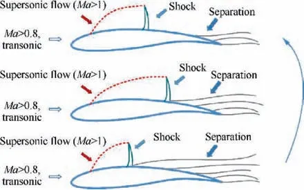
Fig. 17 Schematic diagram of chattering phenomenon in which structure or part of structure undergoes high-frequency irregular vibration due to boundary layer separation or shock vibration.

In applying neural networks to active flow control, Lee et al.made outstanding contributions in this regard. Lee et al.constructed an adaptive controller based on neural network and used it in turbulent flow for drag reduction.The control network executes suction and blowing at the wall based on the wall shear stress in the span direction.The neural network learned the mapping relationship between wall shear stress and wall actuations from the given data set. The result shows that the skin friction of the turbulent channel flow is reduced by more than 20%. It is worth mentioning that the flow control architecture proposed by Lee et al.is an online control method that can adapt to the time-varying and non-linear flow system. The schematic representation of the adaptive inverse model control is shown as Fig. 19.Further on, the neural network scheme proposed by Lorang et al.was used for flow estimation and control in turbulent channel flow with low Reynolds number. The idea is to determine which velocity-length scales are relevant to substantial drag reduction, and how to estimate the flow on these length scales through a sensor grid with a limited range and spacing. The research of Lorang et al. is similar to the research idea of Lee et al. The main difference is that the flow estimation of Lorang et al. is carried out in Fourier space, which allows us to manipulate the wavelength instead of the velocity value in physical space. In terms of reducing the skin-friction drag of the turbulent boundary layer, Mahfoze et al.established a Bayesian optimization framework to optimize the lowamplitude wall-normal blowing control of turbulent boundary layer flow. The Bayesian optimization framework determines the optimal blowing amplitude and blowing coverage to achieve a net energy saving solution of up to 5% in 20 optimization iterations. As shown in Fig. 20,Bayes optimized wall-normal blowing simulation (red solid line) captures the same qualitative and quantitative trends as the reference data(Stroh et al.,red dashed line). The current canonical case without wall-normal blowing is marked by black solid line,while the corresponding data is marked by black box (Schlatter and O¨ rlu¨). Downstream of the control, the skin-friction drag rapidly recovered to the level of no wall-normal blowing,but the significant reduction of skin-friction drag still exists.

In general,using traditional neural network to realize active flow control involves the following three steps: First, a neural network was trained off-line to find the mapping relationship between wall information and wall actuators. Then, based on the network architecture of off-line training, an online adaptive active flow control strategy was implemented. Finally,the weight distribution of the neural network was derived to obtain a simple turbulence drag reduction control architecture.For the use of traditional neural networks to perform active flow control of the flow field,there are still several basic problems that need to be solved. Whether the adaptive controller trained at low Reynolds number can be applied to flow control at high Reynolds number remains to be verified. Another important issue is the impact of the spatial resolution of sensors and actuators on the performance of active flow control remains to be studied.

For the deep dynamic modeling and control of unsteady flow, Morton et al.proposed a method to directly learn the forced and unforced dynamics of the flow on the cylinder surface from CFD data. The proposed method is based on Koopman theory, and the results show that a stable dynamic model can be generated. By using the learned model, Model Predictive Control(MPC)can be performed to suppress vortex shedding caused by cylinder wake. The proposed deep Koopman model is used to learn a state mapping that approximately spans the Koopman invariant subspace. In addition, Efe et al.used neural networks to study the control of cavity flow, which can accurately reproduce the reference signals measured at the bottom of the cavity under different operating conditions.

Generally, neural network can obtain the approximate function between input and output with enough precision because of its strong nonlinear mapping ability.However,neural networks tend to fall into local minima, and pure neural networks can’t interact with the environment, which makes it limited in the actual flow control. In recent years, reinforcement learning, as a ML paradigm that can interact with environment, has attracted more and more attention from researchers, and its application in active flow control is also remarkable.

Fig.18 Response of trailing edge flap angle and lift coefficient of NACA0012 airfoil before and after applying adaptive control in buffet flow.128

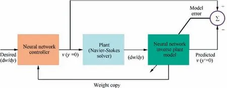
Fig. 19 Schematic diagram of adaptive inverse model control (plant here refers to numerical solver of Navier-Stokes equation, desired wall shear stress is used as input of controller).11

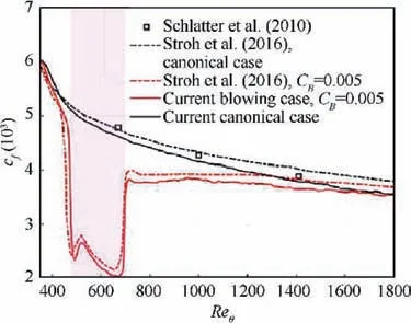
Fig. 20 Changes of skin-friction coefficient with Reynolds number along streamwise for canonical and controlled turbulent boundary layer flow.130

4.1.2. Flow control via reinforcement learning

For the aeronautic industry, designing active flow control strategies is a complicated and laborious task. For easily obtainable measurement values such as pressure or velocity around a given object, it is difficult to find a reliable control strategy for active flow control based on this information.Although considerable efforts have been made in active flow control theory, and various analytical and semi-analyticaltechniques have been used, this bottom-up design method based on flow equations still faces considerable difficulties.Thus,it is necessary to develop more effective control methods to perform complex active flow control. The combination of deep neural network and reinforcement learning has made new breakthroughs in the optimal control of complex dynamic systems,which provides inspirations for its application in optimal flow control.

As Sutton et al.said, reinforcement learning is direct adaptive optimal control. RL builds a formal framework in which an agent learns a series of decisions by interacting with the environment through collecting experience information.The combination of deep learning and reinforcement learning,known as deep reinforcement learning, has made significant progress in the field of active flow control in recent years by exploring high-dimensional nonlinear state space and utilizing the feature extraction capability of deep neural networks.DRL has recently gained widespread application in physics and engineering because of its ability to solve previously difficult decision-making problems due to high dimensionality and nonlinear.

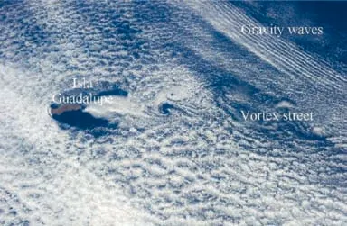
Fig. 21 Ka´rma´n Vortex Street formed on Guadalupe Island(wind blowing from north (left) across island, forming a series of atmospheric vortices in downwind clouds).137

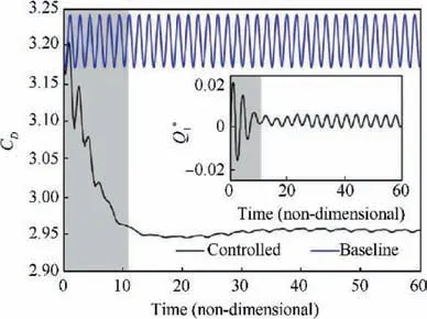
Fig. 22 Schematic diagram of variation of surface drag coefficient CD of a cylinder with(controlled curve)or without(baseline)active flow control over time,and corresponding normalized mass flow rate of control jet (Q*1).138

Using DRL to study the active flow control of Ka´rma´n vortex shedding under moderate Reynolds number is a popular direction. The typical Ka´rma´n vortex street phenomenon in nature is shown in Fig. 21.The neural network based on DRL constructed by Rabault et al.learns the active flow control strategy by conducting experiments on the mass flow rate of the suction and blowing of the nozzle on the side of the cylinder. The effect of applying DRL to control the jet mass flow rate on both sides of the cylinder on the surface resistance is shown in Fig.22.By interacting with the unstable wake, the neural network successfully stabilized the vortex and reduced the drag on the cylinder surface by approximately 8%.Fig.23shows the comparison of the results of applying DRL to control the flow field structure of the cylinder. The inspiration provided by this research is to use Proximal Policy Optimization(PPO)and the fully connected neural network to perform jet flow control on both sides of the cylinder in a twodimensional(2D)simulation.Similar work on active flow control for different Reynolds numbers is also done by Tang et al.The comparison of the drag coefficient of the cylinder with and without the active flow control of DRL is shown in Fig. 24.In addition, Koizumi et al.proposed the use of Deep Deterministic Policy Gradient (DDPG) to control the shedding of the Ka´rma´n vortex street and pointed out that due to the feedback control of the DDPG, the root mean square of the lift acting on the cylinder was reduced.

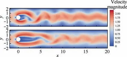
Fig. 23 Comparison of instantaneous flow field around a cylinder without (above) or with (below) active flow.138

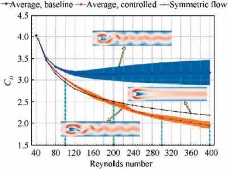
Fig.24 Average drag coefficients of controlled and uncontrolled flows under different Reynolds numbers.139

As far as aerodynamic control devices are concerned, the plasma actuator injects local momentum into the shear layer flow and has the ability to control large-scale flow, which is expected to become an advanced flow control technology to replace traditional vortex generators and mechanical aerodynamic equipment.Accordingly,Shimomura et al.used Deep Q network (DQN) to select the optimal Dielectric-Barrier-Discharge (DBD) discharge frequency in real time, and performed the optimal control of flow separation for an airfoil with an angle of attack of 15°. The control effect of the flow separation on the airfoil surface based on DRL and fixed discharge frequency is shown in Fig. 25.The degree of flow separation is represented by the pressure coefficient Cof the airfoil surface. Furthermore, Gue´niat et al.used a hash function to construct a discrete embedding space and used it for sensor measurement, thereby deriving a Markov process model to approximate the dynamic characteristics of a complex system, and illustrated this idea through the 2D laminar flow of a cylinder, successfully achieved active flow control of oscillating laminar flow around bluff bodies.

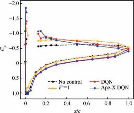
Fig. 25 Cp distribution around airfoil controlled by plasma actuator at angle of attack of 15°.141

In general, deep reinforcement learning algorithms can be roughly divided into value-based method and policy-based method. Among them, the typical representative of the valuebased approach is the DQN. However, considering the shortcomings of value-based methods and policy-based methods,for example,value-based methods are only suitable for scenarios that contain limited actions.A hybrid training method that combines value-based and policy-based methods, namely Actor-Critic is more suitable for complex and changeable scenes such as flow fields. Among them, the most noteworthy is the PPO.Compared with DQN,PPO is more suitable for continuous control problems such as active flow control.Meanwhile,compared with Trust Region Policy Optimization (TRPO), its mathematical form is simpler and faster to calculate.Therefore,the application of PPO should be given priority when applying DRL to study the active flow control of flow field.

In addition to the traditional active flow control mentioned above, some interesting DRL applications are also worthy of attention in biomimetics. Novati et al.used DQN to study the swimming kinematics of two fish-like swimmers in the viscous incompressible flow. The self-propelled swimmer used in the simulation is based on a simplified physical model of zebrafish. The change of swimmer’s body shape is caused by applying a spatiotemporal variation of body shape curvature.The swimming dynamics of multiple self-propelled swimmers implies complex vortex interaction mechanism. The research uses DRL to adapt to the movement of the follower fish to overcome the vortex street generated by the movement of the leader fish. The purpose of this study is to derive a movement strategy that can reduce the energy consumption of follower fish. As shown in Fig. 26, DQNcontrolled self-propelled swimmer has sustained flow patterns and alternate lateral jets due to its systematic interception of wake vortices. However,for uncontrolled followers, no sustained wake pattern was observed. Furthermore, Verma et al.further used DRL to study the swimming strategies of multiple fishes in threedimensional flow. Compared with the research of Novati et al., Verma et al. uses the identical DRL model but adds LSTM to improve the neural network.The author emphasizes the importance of this feature, and past observations include transitions to future actions. The results show that the collective energy saving can be achieved by properly utilizing the wake generated by other swimmers than by multiple individual swimmers.

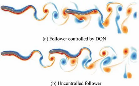
Fig. 26 Contours of vortex interaction with leader’s wake.143

In addition, existing research proposed by Wang et al.also applies DRL to online scheduling of image satellites.Space-based information service requires efficient and fast image satellite scheduling.The existing research considers that image satellite scheduling is an optimization problem solved by batch search algorithm. Wang et al.used DRL and reconstructed the satellite scheduling based on the Dynamic Stochastic Knapsack Problem (DSKP). Numerical results show that the method has good real-time and timely response characteristics.

Generally,the use of DRL to perform active flow control of the flow field is mainly to build a simulation environment,where the agent is responsible for controlling the operation of the actuator,which can be the suction or blowing mass flow rate of the cylinder surface,or the optimal discharge frequency of DBD, resulting the flow field environment changes,and the agent gets feedback to evaluate the effect of the operation performed,and then loops.The idea of feedback control is also the cornerstone of DRL.Since the first edition of Sutton and Barto’s book,RL has become a particularly active area of research.However,the epoch-making prosperity of this field came after the paper of Mnih et al.and its breakthrough in playing Atari games with DQN. So far, countless great achievements have been made in this field, and DRL’s ability to learn complex tasks has been well established. Taking into account the high-level interface of the existing open source library, the coupling of the DRL algorithm and the existing numerical simulation CFD solver can be implemented relatively easily, opening up a wide range of possibilities for optimization and active flow control.However,it is also necessary to realize that although DRL has been proved to be robust in low Reynolds flows, its application in high Reynolds number flows still needs to be realized. So far, the ability and robustness of DRL algorithm in high turbulence and nonlinear flow still need to be explored.

4.2. Neural-free active flow control

There are a wide range of options for neural-free active flow control. For example, open-loop forcing is probably the simplest neural-free control strategy considering its simplicity. In addition, adaptive control can be used as a slow parameter adjustment feedback, wrapped around a working open-loop control to change the behavior of the controller. We focus on the ML-based methods widely used in turbulence control.Neural-free active flow control technologies based on ML,such as Genetic Algorithms (GA) and Genetic Programming(GP), will be introduced in detail in this section. Each method must determine the structure of the control law and identify the parameters of the control law to optimize the control law. The important thing is that neural-free control methods can be applied to numerical or experimental systems with little modification.The current research shows that active flow control based on machine learning can effectively explore and optimize new feedback driven mechanism in many experimental applications.

4.2.1. Genetic algorithm-based control

Evolutionary algorithm is an important type of ML algorithm.For a group of individuals competing in a given task,it spreads the successful strategy to future generations by imitating the optimization process of natural selection.For neural networks,if the problem to be solved has multiple extreme values and the gradient-based algorithm fails,the evolutionary algorithm can usually be used to solve the global optimal solution. For genetic algorithm, evolutionary algorithm is usually used to identify controller parameters. For GA, the initial candidate parameters are called individuals,and the performance of each individual is quantified by a specific cost function in numerical simulation or experiment. After populating individuals in the initial generation, the performance of each individual will be evaluated based on its performance on the cost function.Some individuals with outstanding performance successfully enter the next-generation evolutionary process according to some rules or genetic manipulation.These operations mainly include the following three types: Replication-The selected individuals are copied directly to the next generation; Crossover-The two selected individuals exchange randomly selected values or branch structures, and then evolve to the next generation;Mutation-The partial value or branch structure of some selected individuals will be modified, which has the ability to explore and find a smaller cost function.

According to the above genetic manipulations, the bestperforming individuals in each generation evolve to the next generation, and some new random individuals are added to the population. The evolution process will be until convergence or individual performance meets the desired requirements. Nevertheless, researchers cannot guarantee in advance that genetic algorithms can converge despite their success in a wide range of applications. The accuracy and convergence difficulty of the solution can be controlled by controlling the number of individuals in each generation, the number of generations, and the rate of each gene operation.

Bingham et al.used GA to suppress the fluctuating lift on the cylinder. The Multi-Objective Evolutionary Algorithm(MOEA)was adopted to suppress the change of oscillating lift caused by the vortex shedding of the main cylinder by inserting the control cylinder. The algorithm has two goals, one is to minimize the fluctuating force coefficient of the main cylinder,and the other is to minimize the power to drive the control cylinder.The evolution towards lower oscillating lift and actuator power is shown as Fig. 27. When there are multiple optimization objectives, that is, multiple local minima exist,the algorithm proves that GA can be applied to find multiple optimal solutions at the same time.Moreover,the MOEA proposed by Bingham et al.is suitable for any scenario involving optimizing a fixed number of parameters. Meanwhile,MOEA can determine important parameters autonomously,potentially reducing the complexity of optimizing the search space.In addition,Raibaudo et al.used linear GA to study the control problem of fluidic pinball.The wake stability problem of a triangle group composed of three rotating cylinders is studied. The flow topology of different open-loop control structures is studied, and ML techniques are used to optimize flow control performance. The comparison of the mean streamwise velocity with and without active flow control is shown in Fig. 28. The actuation accelerates the free flow outside the geometric structure and reduces the secondary flow at the centerline. The actuation of the cylinder accelerates the free flow outside the geometric structure and reduces the secondary flow at the centerline. It is worth noting that Milano and Koumoutsakosproposed a clustering GA for cylinder drag optimization,which reduced the drag minimization problem as an optimal adjustment problem. Two ideal actuation forms are considered, one is the ‘‘belt” that moves steadily and tangentially on the surface of a cylinder, and the other is suction and blowing under the constraint of zero net mass.Based on the clustering characteristics of the proposed algorithm, the above two actuation forms are compared and analyzed. More importantly, the presented GA has the characteristic of identifying the smallest basins, rather than identifying the individual best points.What’s more, the actuator parameters of the two-dimensional flow are extended to the three-dimensional flow. The three-dimensional control flow shows strong two-dimensional flow characteristics on the cylinder surface, which significantly reduces the skin-friction of the cylinder.

In addition to the application of GA mentioned above in the field of active flow control,GA are also involved in passive flow control. As a potential passive mechanism to reduce turbulent friction, compliant surfaces have attracted much attention. The main mechanism of drag reduction is the reduction of Reynolds shear stress near the wall caused by surface motion. Based on this principle, Fukagata et al.conducted the DNS of the fully developed turbulent flow in a channel with anisotropic compliant surface, and used GA to optimize the parameters of the compliant surface.Several sets of parameters optimized by GA can reduce skin-friction drag by about 8%. Moreover, to systematically evaluate the proposed compliant surface design, an inverse design optimization program using GA is designed to obtain the optimal parameters of the model.

When the parameter space of flow control is large, traditional open-loop or closed-loop control is very difficult to search. ML can not only be used as a tool to optimize the search in a large parameter space, but also can reveal unexpected solutions or parameter relationships. GA usually involves large-scale parameter identification in a possible highdimensional space,so GA is usually used to adjust the parameters of a predetermined structural control law. For example,GA is used to adjust the parameters of the Hcontroller in the combustion chamber experiment.

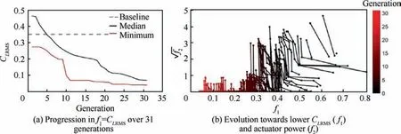
Fig. 27 Objective function changes with generation.146

Fig. 28 Mean streamwise velocity U/U0 for without (left) and with (right) control.147

Generally, compared with the neural network, the convergence of GA needs special attentions. Although GAs have been successfully used in a wide range of applications and mature open source tools are available, and they are likely to converge to the global optimum during training, there is no guarantee that they will converge. There are many ways to improve the performance and convergence of the GA. For example, the number of individuals in a generation, the number of generations, and the rate of each genetic operation determine the quality and convergence rate of the solution of the GA.

4.2.2. Genetic programming-based control

In addition to DRL, GP is also gradually emerging in closedloop control applications of flow separation.GP is a symbolic regression method belonging to the category of machine learning, which was first proposed by Koza.The concept was inspired by GA.GP is used to find the optimal control law that optimizes the cost function.For flow control based on GP,GP is used to iteratively learn and refine the nonlinear mapping from sensors to actuators to achieve certain control purposes.Compared to neural-based flow control using neural networks such as Lee et al.,the output of GP is a functional expression, which allows control laws to be studied and corresponding physical knowledge can be obtained. The genetic manipulation used in GP is shown in Fig. 29. GP detects the nonlinear actuation mechanism in an unsupervised manner, which can be regarded as the generalization of GA in the identification of control law parameters.

The closed-loop flow control in experiments based on GP is still scarce, and the major obstacle is that a large number of experiments are needed to meet the criteria of statistical convergence.Recently,Duriez et al.used GP to find the optimal closed-loop control law in the flow control problem. Moreover, for Backward-Facing Step (BFS) flow, Gautier et al.used GP to reduce the recirculation area of the BFS flow at a Reynolds number of 1350 through a slit jet, and obtained the flow field changes through real-time PIV optical perception.The flow control is driven by an upstream jet with a spanwise slot. The specific control law is derived from genetic programming. The results indicate that the feedback control law obtained by GP can reduce the recirculation area by approximately 80%. Moreover, research by Gautier et al.demonstrated that GP can resolve the problem of multi-input/multi-output. By adding the output of the controller and the input of the sensor,it can provide more freedom for the system to reduce the cost function. For example, the time delay and the derivative of sensor information can be input into the model to allow the embedding of dynamic systems. The schematic representation of active flow control process based on GP is shown in Fig. 30. In addition, Debien et al.conducted closed-loop control of the turbulent boundary layer separated downstream of sharp edge ramp through experiments where the feedback control law was obtained by GP. The purpose of the control was to mitigate separation and early re-attachment. The control was introduced by the active vortex generator, and the flow condition was evaluated by momentum coefficient, pressure distribution, skin-friction and stereo PIV.

Similarly, Li et al.used linear genetic programming to study the closed-loop control of aerodynamic drag reduction of a car model. The actuation is driven by pulsed jets, and the flow configuration is monitored by pressure sensors. The optimized control law includes periodic forcing, multifrequency forcing and sensor-based feedback, as well as time history information feedback and its combination. For the optimized control law, approximately 33% of base pressure recovery and 22% of drag reduction can be achieved, indicating that linear genetic programming is a powerful regression technique for optimizing multiple input and multiple output control laws. Current research shows that ML based control strategies can effectively explore and optimize new feedback mechanisms in many experimental applications.

Combining the above researches, it can be found that the main advantages of the active flow control based on GP are efficiency and robustness. Since it is not model-based and can virtually generate any type of control laws (linear or non-linear), this makes the GP-based method can be used to study the flow of specific geometric configurations,such as turbine blades or vehicle model.

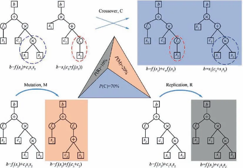
Fig. 29 Genetic manipulation used in GP to improve function of generations.152

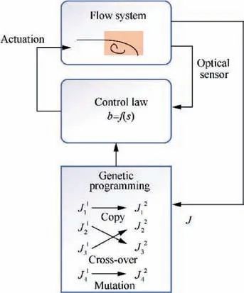
Fig. 30 Control loop featuring genetic programming (control laws b=f（s） are evaluated by flow system; new generations are produced by replication, cross-over and mutation; represents the ith individual of the nth generation).154

Fluid-Structure Interactions (FSIs) problems are ubiquitous in actual engineering applications, e.g. bridges that vibrate up and down in typhoons, the air flows through the blades of the wind turbine, long pipeline to carry oil. Vortex-Induced Vibrations (VIVs) is a special type of FSI problem,which involves resonance conditions. For the external fluid passing through the bluff body, the VIVs will be caused when the frequency of vortex shedding on the surface of the bluff body is close to the natural frequency of the bluff body.For the problem of VIVs,a prototypical example is fluid passing through the circular cylinder, causing the so-called Ka´rma´n vortex shedding when the Re ＞ 47. Traditional Computational Fluid Dynamics (CFD) technology can be used to accurately simulate the flow passing through the bluff body and the movement of the structure. However, CFD simulation is limited to low Reynolds number and simple geometric configuration, and involves complex boundary mesh shape changes. In recent years, some methods of using GP to suppress VIVs are worthy of attentions. Ren et al.used GP to select explicit control laws to suppress VIVs at low Reynolds numbers in the data-driven and unsupervised manner by means of suction or blowing. From the open-loop control knowledge of purely suction or blowing, a loss function is designed to balance the suppression of VIVs and energy consumption. To further evaluate VIVs control based on GP,the authors compare the optimal controller based on GP with traditional linear control techniques such as Proportional Integral Differential(PID)control.The optimal control law generated by GP suppressed 94.2% of the VIVs amplitude, and the overall performance was improved by 21.4% compared with the optimal open-loop control. Moreover, the control law selected by GP is robust and effectively suppresses the VIVs in the Reynolds number range of 100-400. The jet velocity of the best control law selected by GP and the displacement of the cylinder are shown in Fig.31.It should be noted that due to the randomness of the initial population and the mutation in the evolutionary process, the mathematical expression of the optimal control law generated by each training of GP is not necessarily the same.

For the use of deep neural networks or GP to study FSIs problems, there is no need to specify geometric configurations or set boundaries or initial conditions as traditional numerical methods. In addition, among the methods discussed here, GP is the only method that can identify both the structure of the control law and the parameters of the control law. What’s more,while many ML methods such as support vector machines, random forests, Gaussian processes,and neural networks merely act as black box, researchers in the field of fluid mechanics should open the black box to understand the internal mechanisms and discover new technologies that are more suitable for fluids.

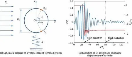
Fig. 31 Schematic diagram of vortex-induced vibration system and effect of active flow control.158

Generally,the effect of applying GP to the active flow control of the flow field is significant,and it provides better robust performance under extremely nonlinear conditions. However,for the control of complex dynamic systems, there are also some unexplored and extensible problems with GP. In actual situations, due to high computational costs or rough experimental measurements, it may be difficult for GP to find sufficiently reliable data. In addition, for GP, the input of the control law can be considered to be composed of suitable time periodic functions, so that the open-loop actuations can be optimized.

The ML-based approach to active flow control discussed above is a very general approach, including open loop and closed loop control. Although the resulting controller may achieve global cost function minimization, convergence is not guaranteed and depends on the dimensional size of the input space. Compared with the active flow control methods based on neural networks, the neural-free control methods such as GP or GA are more suitable for the situations where the parameter space is small or the explicit control law is needed.Actually, the neural-based control methods are essentially the feedback-based that interact with the flow field environment,while neural-free control methods are essentially evolutionary algorithms. In terms of complexity of learning task and learning speed, active flow control methods based on neural networks are better than neural-free methods such as GP or GA. The research content and methods of active flow control using ML such as DRL or evolutionary algorithms are summarized in Table 3.

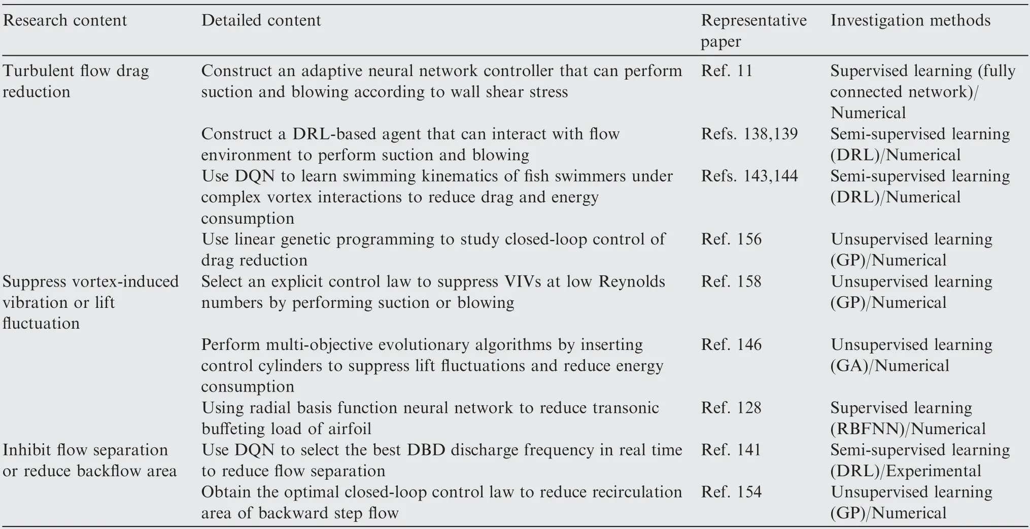
Table 3 Summary of active flow control based on machine learning

5. Conclusions

This review provides applications and opportunities for ML algorithms in fluid mechanics. The convergence of two seemingly unrelated disciplines has had a long and tortuous history.This review briefly introduces the applications of ML algorithms in flow modeling, reconstruction and prediction, and active flow control in experiments and simulations.It discusses in depth the bright spots and shortcomings of these applications, and can prove that the current research trend with the development of technology is of great benefit. Our purpose is to provide readers with different backgrounds with a deeper understanding of ML algorithms in different fluid mechanics contexts. The following conclusions can be extracted from the articles reviewed above:

(1) ML algorithms provide a library of tools suitable for different application contexts. These tools have not yet maximized their effectiveness in fluid mechanics and can enhance existing research models. This knowledge of data mining and pattern recognition can help build more accurate problem models and help reduce the computational cost in turbulence calculations and active flow control problems. For example, ML algorithms can provide a way to search and visualize highdimensional nonlinear feature spaces. The traditional flow control strategy mainly includes from the understanding of the physical mechanism to modeling and then to control. ML algorithms provide more flexible strategy choices for flow control.

(2) In the near future, ML algorithms will help expand the linearization model of fluid mechanics problems and the linear method of nonlinear problems. Two factors make it possible to train these complex models based on ML.The first is the proposal and application of automatic differentiation and backpropagation algorithms,especially the ease of programming. The second factor is the improvement of computing power,such as the proposed computing framework and the application of modern graphics processing units.A large number of ML open source software frameworks such as TensorFlowand PyTorchand community communications have lowered the research threshold for researchers in the field of fluid mechanics,and promoted the process of integrating ML and fluid mechanics. In the long run, ML will undoubtedly bathe in the light of big data and provide new research perspectives for the old problems of fluid mechanics.

(3) In recent years, deep learning, as the most attractive algorithm in machine learning, has made remarkable achievements in flow modeling and other aspects. However, deep learning cannot completely replace machine learning. When selecting specific methods in practical application, one should not excessively pursue the fashion of methods, more attentions should be paid to data preprocessing and quantity size, input and output of sample pairs, cost functions in specific tasks, and interpretability of models.

(4) Fluid mechanics is traditionally a data-rich subject, but it is more expensive to obtain data in many contexts. In addition, the fusion of ML and fluid mechanics will inevitably require relevant practitioners to have a professional background in ML and a deep knowledge of fluid mechanics.Moreover,ML encourages open source data and code,and the development of a ML framework suitable for fluid mechanics is also a focus of attention.In general, DNN results should never be trusted unless strict cross-validation has been performed. Crossvalidation plays the same critical role as the convergence of numerical simulation.

(5) More importantly,the application of neural network also needs to be treated from two aspects.For some simple and direct applications such as face recognition, the existing algorithms are very mature, and the remaining work is mainly for engineers rather than researchers. For the application of neural networks to other subjects such as fluid mechanics,the key to the problem is not the neural network itself, but the presentation and transformation of the problem, the preparation and pre-processing of data, and the analysis and application of the output results.

(6) Flow control strategies have traditionally been based on a precise sequence from understanding flow conditions to modeling and then to control. The paradigm of ML, especially reinforcement learning, provides more flexibility and iterative methods on a data-driven basis.

The authors declare that they have no known competing financial interests or personal relationships that could have appeared to influence the work reported in this paper.

s

This research work is supported by the National Natural Science Foundation of China (No. 11972139). Moreover, the authors wish to thank the reviewers for their insightful comments.