Pressure distribution feature-oriented sampling for statistical analysis of supercritical airfoil aerodynamics

Runze LI, Yufei ZHANG, Haixin CHEN

School of Aerospace Engineering, Tsinghua University, Beijing 100084, China

KEYWORDS Adaptive sampling;Output space;Statistics;Pressure distribution features;Supercritical airfoil

Abstract In the field of supercritical wing design, various principles and rules have been summarized through theoretical and experimental analyses. Compared with black-box relationships between geometry parameters and performances, quantitative physical laws about pressure distributions and performances are clearer and more beneficial to designers. With the advancement of computational fluid dynamics and computational intelligence,discovering new rules through statistical analysis on computers has become increasingly attractive and affordable.This paper proposes a novel sampling method for the statistical study on pressure distribution features and performances, so that new physical laws can be revealed. It utilizes an adaptive sampling algorithm, of which the criteria are developed based on Kullback-Leibler divergence and Euclidean distance.In this paper, the proposed method is employed to generate airfoil samples to study the relationships between the supercritical pressure distribution features and the drag divergence Mach number as well as the drag creep characteristic. Compared with conventional sampling methods, the proposed method can efficiently distribute samples in the pressure distribution feature space rather than directly sampling airfoil geometry parameters. The corresponding geometry parameters are searched and found under constraints,so that supercritical airfoil samples that are well distributed in the pressure distribution space are obtained. These samples allow statistical studies to obtain more reliable and universal aerodynamic rules that can be applied to supercritical airfoil designs.©2021 Chinese Society of Aeronautics and Astronautics.Production and hosting by Elsevier Ltd.This is an open access article under the CC BY-NC-ND license(http://creativecommons.org/licenses/by-nc-nd/4.0/).

1. Introduction

Supercritical airfoils offer superior performance for transonic flight, including a larger cruise lift to drag ratio (L/D), a delayed drag divergence Mach number, and a large volume for structure and fuel storage.These benefits can be attributed to the airfoil’s performance in terms of establishing an appropriate pressure distribution, which balances the shock wave’s drag penalty and its benefits toward pressure recovery,striking a compromise between lift generation and the Mach number in front of the shock wave.The complexity of the pressure distribution lies in the nonlinear and sensitive nature of transonic aerodynamics, which is caused by the on-body shock wave and its interaction with the boundary layer.

Over the past 60 years,many researchers have both theoretically and experimentally studied the relationships between airfoil performance and flow features, such as pressure distribution features and surface separations. Their work has significantly contributed to aircraft design. Korn’s equationdescribes the growth of the shock wave relative to the free-stream Mach number and further states the relationship among the thickness, drag divergence Mach number, and lift coefficient. Oswatitsch’s theorem shows that the wall Mach number in front of a shock wave can be used to estimate wave dragand improve optimization efficiency. Zhang et al.manipulated the pressure gradient of the suction plateau on supercritical natural laminar flow airfoils to control the length of the laminar flow region. Pearceystudied the incipient separation on airfoil surfaces,which occurs when a reverse flow is imminent in the boundary layer. Pearcey found that incipient separation occurred when the shock wave reached a certain strength. Furthermore, the size of a shock wave-induced boundary layer separation was also studied to predict the buffet onset lift coefficient, and the spanwise location of the separation was found to contribute to the buffet severity. In combination, these studies have revealed the impact of flow features on performance and showed the importance of ‘‘flow feature-performance” relationships in aircraft design.

These ‘‘flow feature-performance” relationships have been mostly concluded based on theoretical or experimental studies of several typical conditions and samples. With the development of Computational Fluid Dynamics (CFD), CFD-based statistical research has started to gain additional attention.Emerging technologies such as machine learning and data mining can help researchers effectively obtain desired samples for subsequent analysis. Currently, researchers have exploited CFD data via surrogate models in aerodynamic optimizations. These machine learning-assisted methods, e.g.,surrogate-based optimization methodsand data-driven approaches, typically utilize data to predict aerodynamic performance based on the geometry of a wing or an airfoil.But for supercritical airfoils, due to the complexity of nonlinear transonic aerodynamics,slight changes of the airfoil geometry can cause significant changes of its pressure distribution and performance.The relationship between geometry and performance is usually so complicated and incomprehensible that can only be described by black boxes. Therefore, rather than these black boxes,it is the brief and comprehensive laws about pressure distributions,e.g.,the Oswatitsch’s theorem and Pearcey’s law about incipient separation,that are more valuable to engineers.

In order to discover new relationships between pressure distribution and performance, airfoil samples with different supercritical pressure distributions are needed. As shown in Fig. 1, the flow features (including pressure distribution features) are extracted from the CFD result of a specific geometry, and the performances are the physical outcome of flow features. Then, the geometry parameters are represented by the input vector x, and the flow features and performances are represented by the output vector y and Y, respectively.

Fig. 1 Geometry, flow features, and performances.

Conventional sampling methods are designed to properly distribute samples in the input space or to improve the approximation of relationship x →y（orY）. Therefore, the conventional sampling methods tend to generate airfoil samples with various geometries regardless of their pressure distribution.Simply sampling airfoil geometries can neither guarantee the samples having supercritical pressure distributions,nor control the sample distribution in the output space of y. This is a new challenge for which the conventional sampling methods are not designed.

This paper proposes a novel Output Space Sampling(OSS)method that utilizes an adaptive sampling algorithm to generate supercritical airfoil samples with different pressure distribution features. Then, by generating airfoil samples with well-distributed pressure distribution features,the correlations between the shock wave and several airfoil performances are studied statistically.

This paper is organized as follows.First,the relevant background is discussed. Second, the output space sampling algorithm is described, and several sampling criteria are proposed for either improving the output space-filling property or exploring the output space boundaries. The OSS method is then compared with other sampling methods by analytical test functions. Third, the OSS method is used to generate airfoils with various pressure distributions, and the OSS method can obtain more valid supercritical airfoil samples. Finally, these samples are statistically studied. The results are discussed and found to indicate that the drag divergence Mach number increases when the airfoil has a more upstream shock wave,and the drag creep characteristic may deteriorate if the suction peak is too high.

2. Output space sampling method

Sampling methods are essential tools for statistical studies and data mining. Conventional sampling methods usually aim either to fill the input space with uniformly distributed samples or to distribute samples in the input space according to a specified probability density distribution so that the samples are valid for statistical studies of x →y. However, when conducting statistical studies regarding the relationships between y and Y as shown in Fig. 1, the distribution of y is the focus.

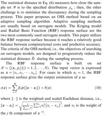
This section begins with stating the difference between sampling the inputs and outputs,which indicates that a novel sampling method is needed for output space sampling. This presents two challenges for OSS.The first challenge is to measure how close a sample set is to the specified distribution p,which is addressed in Section 2.2 by introducing a statistical distance measure ～D .The other is to develop an adaptive algorithm to minimize the discrepancy between the samples and the specified distribution pduring the sampling process, which is introduced in Section 2.3.Then,the OSS method is tested and compared with other sampling methods using several analytical functions.In this paper,the probability density and sample density are denoted as p to distinguish them from pressure p.

2.1.Difference between sampling in input space and output space

Sampling methods can be roughly categorized into stationary and adaptive sampling methods. Stationary sampling methods solely focus on the input space and usually generate samples from several common distributions, such as uniform distribution and Gaussian distribution. The improved Latin Hypercube Sampling (iLHS) method is a modified version of the commonly used Latin hypercube sampling stationary method, which can sufficiently fill the input space with evenly distributed samples in most situations. For other distributions,there are also stationary methods such as rejection sampling, which can generate samples from any specified probability distribution.On the other hand,adaptive sampling methods typically begin with a relatively small number of initial samples generated by stationary methods,and then new samples are sequentially added based on several criteria.Adaptive sampling methods usually utilize surrogate models to find the proper new samples in iterations. Many criteria are designed to most effectively improve the surrogate model rather than generate samples from a specified distribution.

Nevertheless,these methods are designed to distribute samples in the input space, in which the values of the samples can be directly assigned.However,even though the input distribution can be manipulated according to a specified distribution,the distribution of the outputs is not controlled. For example,considering a scaler function y=x(x ∈［0，1 ］),the density distribution of y is not the same as x for one set of ｛x，y ｝samples.Figs. 2(a) and (b) show the rescaled histograms of 2000 samples representing their density distributions (p) in the output space and input space. The samples are evenly distributed in the input space and output space. The height of each bin in the rescaled histogram is the proportion of samples that fall in that interval to the entire set so that the total area of bins is one. Fig. 2 indicates that it is not straightforward to obtain｛x，y ｝samples so that y of these samples conforms to a certain distribution.

Therefore, it is difficult to design a sample set Y= ｛y｝(i=1，2，···，N) in the output space Dwhen the output y is evaluated from a function of input x, i.e., f（x ）. This is especially true if the samples are required to be distributed according to a specified probability density distribution p（y ） (The output space D⊆R, nis the output dimension). Although a hypothetical sample set Y= ｛y｝ can be sampled from pusing rejection sampling, the corresponding input xmust be found for every y; otherwise, there is no guarantee that yis mathematically reasonable. In other words, it may not always be able to find an x∈Dfor any y∈Dthat has y=f（ x） (The input space D⊆R, nis the input dimension).Therefore,the sampling in the output space is more complicated than that in the input space.

An inverse approach is the intuitive choice,which is to find xfor each yin the hypothetical sample set Yby solving x=f（y ）. However, it is impossible to analytically solve the inverse function ffor most functions,and it can also be very computationally inefficient for numerical approaches to find the corresponding xfor each y. Therefore, a direct method is needed, which finds a sample set X= ｛x｝, and the output sample set Y= ｛y｝ is then evaluated with function f afterwards. One challenge is to measure how close the sample set Y is to the specified distribution p, and the other challenge is to develop an algorithm to minimize the discrepancy during the sampling process.

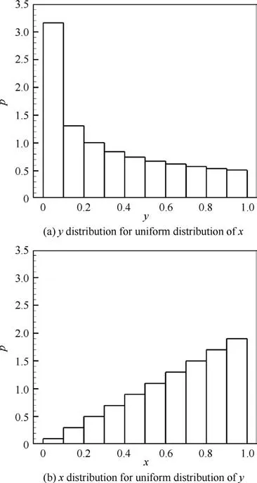
Fig. 2 Histogram of samples in input and output spaces.

2.2. Measuring distribution of samples in output space

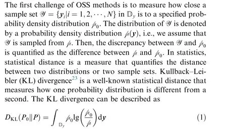
where P and Pare the continuous probability, and p and pdenote the probability densities of P and P, respectively.

The KL divergence Dis always nonnegative, and it will decrease to zero if and only if the two distributions are identical almost everywhere.Then,according to Monte Carlo integration, Eq. (1) can be estimated by Eq. (2) when m is very large. E［·］ represents the expectation of the function inside square brackets according to p.y(j=1，2，···，m)are points sampled according to p.These points are called targets in this paper because they are used as targets for the OSS method to generate samples around these locations.

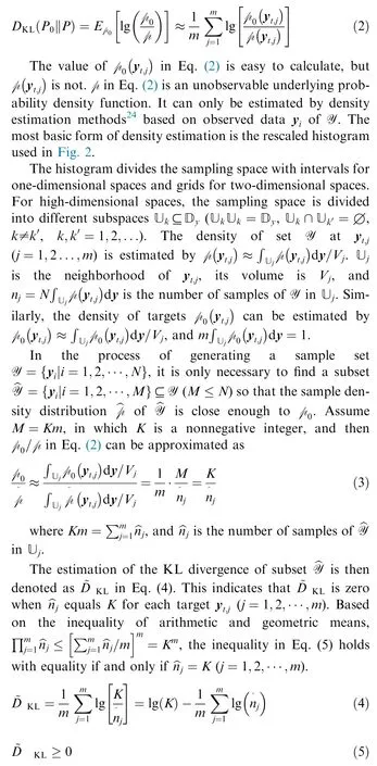
Eq. (4) enables the estimation of KL divergence by the number of samples in the neighborhood of targets, which is much simpler to implement than using other density estimation methods. For example, apart from histograms, there are methods such as multivariate kernel density estimationthat can estimate the high-dimensional probability density functions so that the KL divergence in Eq. (2) can be evaluated accordingly. However, this approach creates high computational costs for building the multivariate kernel density estimation, and it is difficult to develop the OSS method within this scenario.

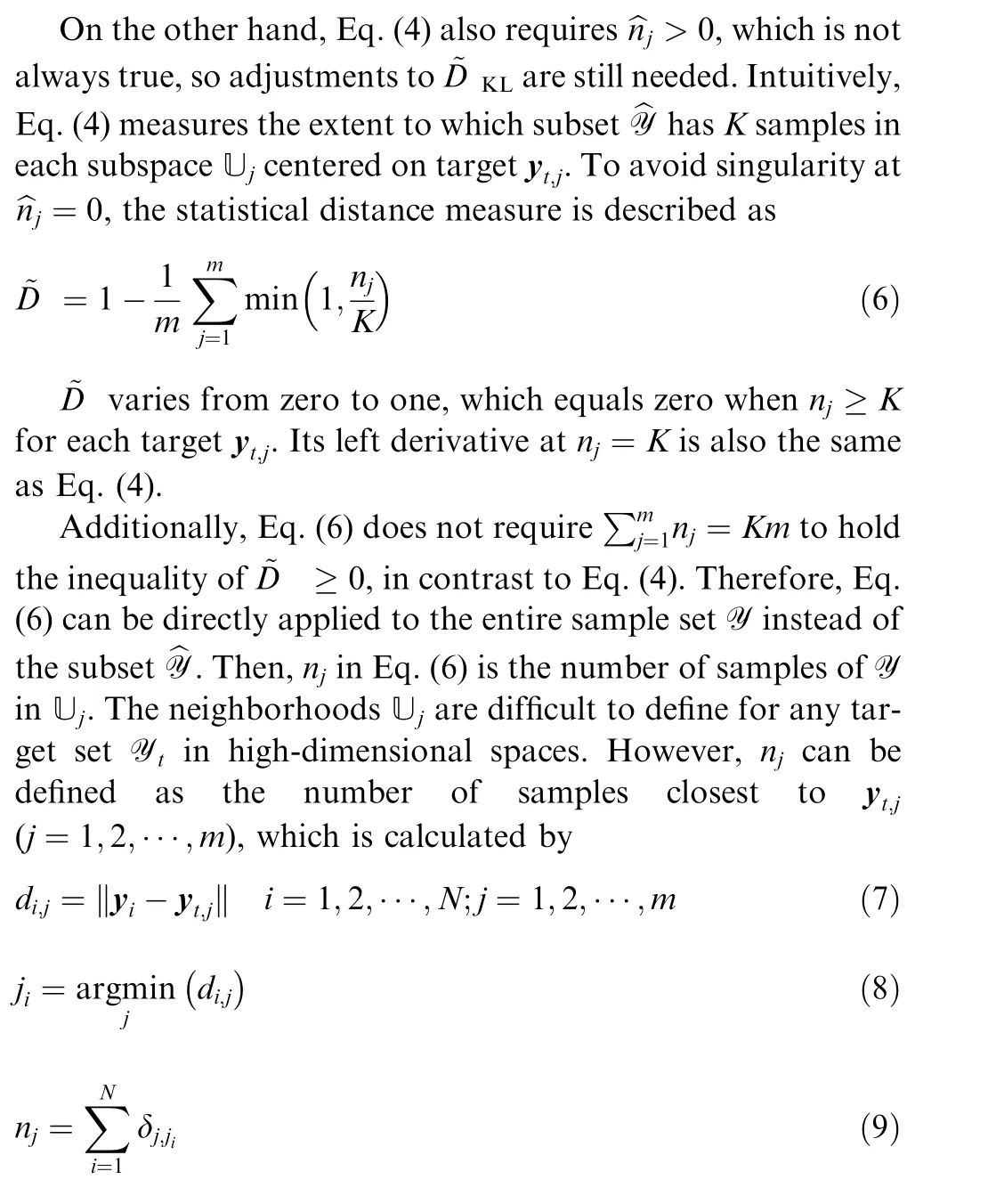
where dis the Euclidean distance between sample yand target y.jis the index of targets to which sample yis the closest.δin Eq. (9) is the Kronecker delta, which equals one when j=j; otherwise, it equals zero.

2.3. Algorithm of output space sampling method

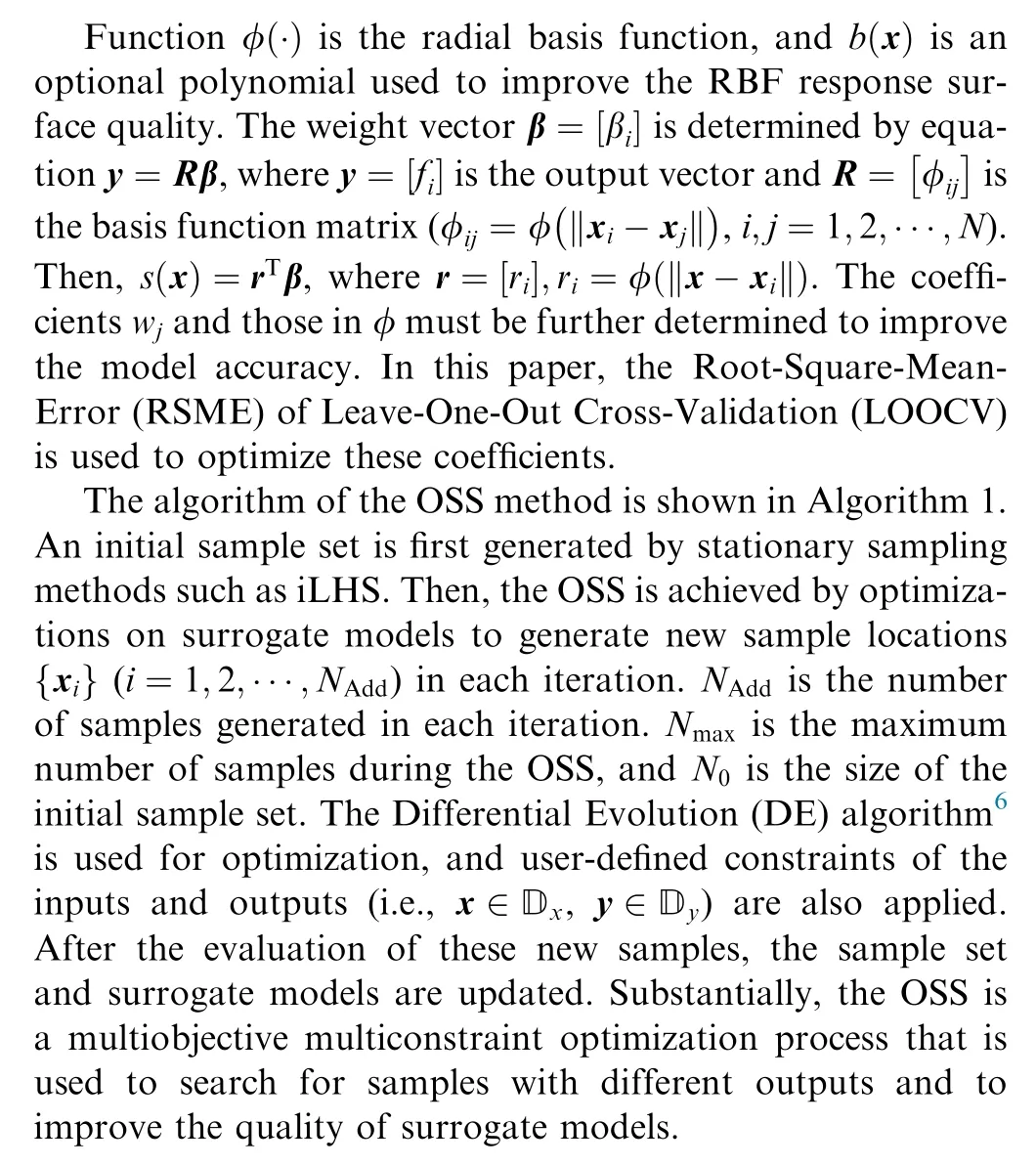
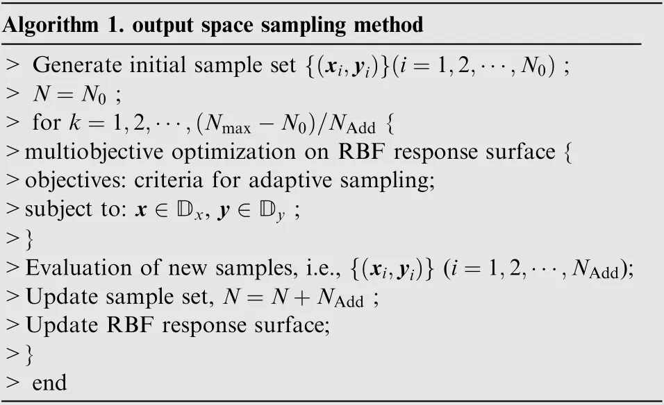
Algorithm 1. output space sampling method＞Generate initial sample set ｛（xi，yi）｝ i=1，2，···，N0） ;＞N=N0 ;＞for k=1，2，···， Nmax-N0（（ ）/NAdd {＞multiobjective optimization on RBF response surface {＞objectives: criteria for adaptive sampling;＞subject to: x ∈Dx, y ∈Dy ;＞}＞Evaluation of new samples, i.e., xi，yi｛ ｝ (i=1，2，···，NAdd);＞Update sample set, N=N+NAdd ;＞Update RBF response surface;＞}＞end（ ）

To generate multiple samples in each iteration,i.e.,N>1 in Algorithm 1, two criteria are typically used as objectives for the optimization. New samples are selected from the Pareto front of the final solutions. In addition, the initial population of the multiobjective optimization can be selected from the existing samples, which tends to increase optimization efficiency on surrogate models rather than randomly generate the initial population.

The most important part of adaptive sampling is to employ proper criteria,i.e.,the objectives of the optimization of surrogate models. There are usually three categories of criteria utilized in the OSS method, i.e.,to improve the surrogate model,to explore the most unexplored region of the input or output space,and to obtain the samples that conform to the specified distribution.

Several criteria for exploring and improving RBF response surfaces have been developed for adaptive sampling, e.g., the separation function and Laplacian function.The minimum Euclidean distance criterion,d（x ）in Eq.(11),can achieve comparable results with much cheaper computational costs.

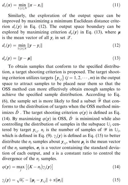
In summary, the OSS method is designed to address three main challenges in the statistical studies of outputs. The first challenge is to indirectly sample the outputs y by finding the corresponding x, which is achieved by searching on the surrogate models. The second challenge is to generate samples according to a specified sample distribution pwhen constraints of samples are given. This is solved by generating the targets and maximizing the criterion φ（y ） in Eq. (14), and the constraints are included in the optimization of surrogate models.The third challenge concerns the output space boundaries. Sometimes the output space-filling property requires improvement, but the output space boundaries must also be explored because they cannot be known beforehand. Then,the d（y ） criterion in Eq. (13)can be employed to address this challenge.

2.4. Analytical test of obtaining specified distributions

Three functions with scaler input and output and one function with scaler output are used in this section. They are employed to test the ability of the OSS method to generate samples in the output space according to a specified density distribution p.The specified distributions are Gaussian distributions with different mean values (μ) and standard deviations (σ). The test functions and specified distributions are listed in Table 1.Twenty targets are generated according to the Gaussian distribution and used for the OSS method, and 100 samples are to be distributed according to the specified distributions. In the first three cases, the OSS method starts from 20 evenly distributed samples in the input space.In the fourth case,it starts from 20 samples generated by the iLHS method in the input space. Two samples are added to each iteration using criteria d（x ） and φ（y ） in Eq. (11) and Eq. (14).

During the sampling process, not all the samples are valid to form the specified distribution, i.e., only some of the samples are selected as the desired 100 samples. The OSS method stops when the statistical distance ～D from the valid samples to preaches zero,which indicates that the number of valid samples reaches 100. Consequently, the total number of samples generated by the OSS method is not the same in the four cases;they are 124, 138, 142, and 156. In contrast, it takes 186, 148,192, and 468 samples to make ～D reach zero when adaptive sampling in the input space is employed. The adaptive sampling method is also based on RBF response surfaces, and d（x ） in Eq. (11) and the Laplacian functionare used as criteria. The results show that the OSS method has higher efficiency in distributing samples in the output space, especially in high-dimensional spaces.

Figs.3-6 show the density distributions of four test cases,in which the density distributions of samples are estimated by the density estimation method with Gaussian kernels.The black solid curves are the specified distributions in Table 1. The green dashed curves are the density distribution of the 100 valid samples in the input space and the output space, which shows that the valid samples are indeed distributed according to p, which proves the sampling ability of the OSS method.The green solid curves are the density distribution of all the samples generated by OSS, although they are not the same as valid samples;the closer they are,the fewer invalid samples that are generated and the higher the sampling efficiency is.The contour flood in Fig. 6 shows the value of y ; the isoline is the density distribution of valid samples in the twodimensional input space, the solid scatters are valid samples,and the empty scatters are invalid samples.

The last three cases show that OSS can generate samples according to the specified distribution in the output space; in addition, the multiobjective optimization with d（x ） and φ（y ）criteria can also diversify samples in the input space when there are multiple solutions of x=f（y ）.

2.5. Analytical test of filling output space

With the proposed criteria, the OSS method can explore the output space, whereas stationary methods such as iLHS just fill the input space. The OSS method is tested on a twodimensional function, and its results are compared with other stationary or adaptive sampling methods. The test function is described in

Table 1 Test functions and specified distributions.

which shows a circle output space for a square input space.In most situations, the actual shape of the output space is unknown; therefore, to fill the output space, the specified distribution is a uniform distribution in the two-dimensional square, y ∈［0，1 ］.

Four cases are tested on this function, for which 400 samples are generated and plotted in Fig. 7. The iLHS method is the baseline sampling method, and the adaptive sampling method using criteria d（x ）in Eq.(11)and the Laplacian functionrepresent the conventional adaptive sampling method.The OSS-1 case employs OSS with the Euclidean criteria d（x ） and d（y ） in Eq. (11) and Eq. (12), and the OSS-2 case uses the criteria d（x ）+d（y ） and φ（y ） in Eq. (11), Eq. (13)and Eq.(14).The four cases all start from the same initial sample set which contains 100 samples generated by the iLHS method. For Cases 2, 3, and 4, four samples are generated in each iteration.Since the specified distribution is a uniform distribution in y ∈［0，1 ］, 100 targets generated by the iLHS method in y ∈［0，1 ］are used in Cases 3 and 4. The histories of the four samplings and the theoretical lower bound of ～D(Eq.(6))are shown in Fig.8 and Table 2.Since the actual output space is a circle,the specified distribution is defined on the square y ∈［0，1 ］.According to Eq. (6), only the targets inside the circle can achieve n≥K,which is π/4 ≈0.79 of the square space y ∈［0，1 ］.The other targets can only have n=0.Therefore, the theoretical lower bound of ～D is 1-π/4 ≈0.21.

The results show that the iLHS method generates evenly spread samples in the input space, and thus the samples only cover a part of the output space. The adaptive sampling method can explore the output space to a certain extent, but the boundaries are not explored. In contrast, the OSS method can not only fill the output space but also explore the boundaries by using different criteria. The OSS-1 case explores the input and output spaces, which has a similar effect as that of the conventional adaptive sampling methods. The OSS-2 case uses the d（y ） criterion to explore the output boundaries and the φ（y ） criterion to fill the output space, and it achieves the best space-filling property with a higher convergence rate.

Then, the OSS method is compared with the iLHS method on the test function in Eq.(17).It can be seen that the inequality in Eq. (18) holds for yand y.

To study the relationship between yand y, the specified distribution for the OSS method is a uniform distribution in y∈［0，1 ］.The OSS starts from an initial sample set of 40 samples generated by the iLHS method;two samples are generated in each iteration, and the criteria are d（x ）+d（y ） and φ（y ）.Twenty targets are evenly distributed in y∈［0，1 ］,and a total of 100 valid samples are desired for the nonlinear regression of y-y.

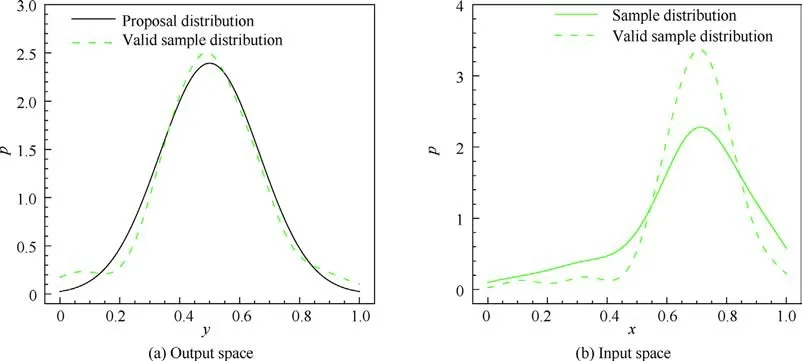
Fig. 3 Sample distributions of y=x2

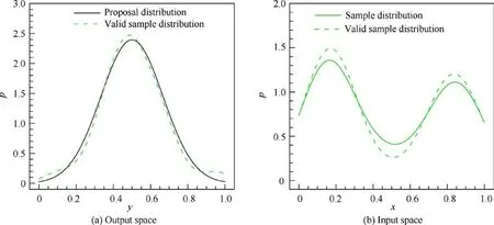
Fig. 4 Sample distributions of y=sin（πx ）

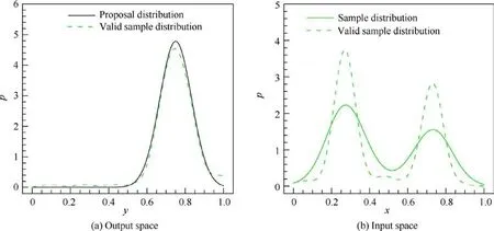
Fig. 5 Sample distributions of y=sin（πx ）

It takes 190 samples for the OSS method to generate 100 valid samples, which are plotted as green squares in Fig. 9.Then,the iLHS method is employed to generate 190 samples in the input space, of which the outputs are plotted as black triangles in Fig. 9. These samples are used for nonlinear regression with the sixth-order polynomic functions. The fitting curves are plotted as dashed curves in Fig.9.The result shows that the iLHS method cannot distribute the samples throughout the entire output space of y,and thus the regression overfits the data in a partial range. In contrast, the 100 valid samples generated by the OSS method are evenly distributed in the yspace,which in return ensures the accuracy of the regression of y-y.

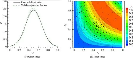
Fig. 6 Sample distributions of y=sin（π x1x2）

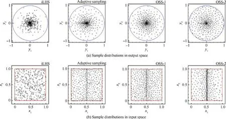
Fig. 7 Sample distributions of four cases.

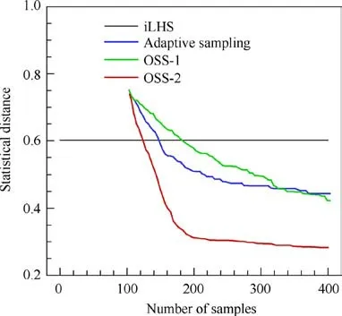
Fig. 8 History of statistical distance.

In summary, the OSS method can effectively distribute samples in the output space according to specified distribu-tions.The output space boundaries are explored,and the sample input is also diversified for the same output.Therefore,the samples generated by the OSS method are more suitable for further statistical studies since they have a higher probability of avoiding bias in the sample set or overfitting the data.

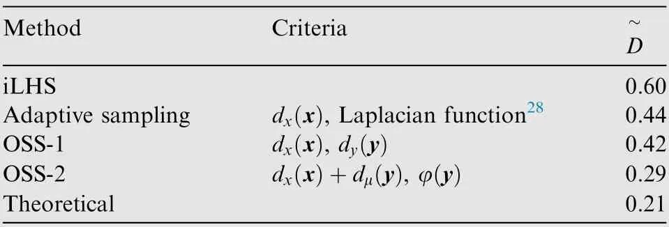
Table 2 Criteria and statistical distances of four methods

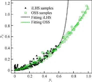
Fig. 9 Nonlinear regression of samples from iLHS and OSS.

3. Statistical study of supercritical airfoils

Korn’s equation identifies the connections among the drag divergence Mach number Ma, lift coefficient Cand airfoil maximum thickness （t/c ）at transonic speeds, which is described as Ma+0.1C+ （t/c ）=κ. κ represents the airfoil technology level of different airfoils. For NASA supercritical airfoils, κ is approximately 0.95, and it shows a good estimation at lift coefficients of approximately 0.4 and 0.7.

Korn’s equation shows a simple linear correlation between Ma, Cand （t/c ）; however, the parameter κ raises a question regarding the influence of other airfoil features that must be answered. Because the flight performances of supercritical airfoils at transonic speeds are significantly affected by pressure distributions, their influences on the technology level κ must be further studied.

This section employs the OSS method to generate supercritical airfoils of the same （t/c ）,C,same shock wave strength and similar lower surfaces to study the influence of shock wave location and suction peak.Their effects on the drag creep characteristics are also studied.

3.1. Airfoil parameterization and CFD methods

The Class Shape function Transformation (CST) method is selected to generate the airfoil geometry. The CST method combines class functions and shape functions to describe an arbitrary geometry and can guarantee airfoil smoothness with comparatively fewer design variables. A sixth-order Bernstein polynomial is used as the shape function, i.e., seven CST parameters are used to describe the upper and lower surfaces.

A C-grid is employed for Reynolds-Averaged Navier-Stokes (RANS) analysis. The CFD solver is a well-known open source solver named CFL3D.In this paper,the MUSCL scheme, Roe’s scheme, the lower-upper symmetric Gauss-Seidel method, and the k-ω Shear Stress Transport (SST)model are selected for reconstruction, spatial discretization,time advancement, and turbulence modeling, respectively, in RANS. The CFL number is 2.0 for 5000 steps.

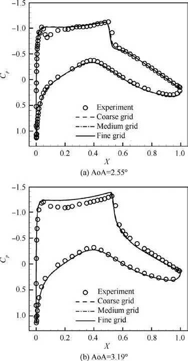
Fig. 10 Grid convergence study of Cp

Fig.10 shows the experimental pressure coefficient(C)distributions of an RAE2822 airfoilcompared with the CFD results of different grid sizes. Two flight conditions with weak and stronger shock waves are used for validation. Fig. 10 (a)shows that the free-stream Mach number (Ma) is 0.725, the Reynolds number (Re) based on the unit chord length is 6.5×10, and the Angle of Attack (AoA) is 2.55°. Fig. 10(b) shows that Mais 0.73, Re is 6.5×10, and AoA is 3.19°. The three grids, with sizes of 20000, 40000, and 80000,have 201, 301, and 401 grid points on the airfoil surface,respectively.Δyof the first grid layer is always kept less than 1. All grids can achieve a similar Cresolution for both cases.The medium grid is employed in this paper.

3.2. Key pressure distribution features

The performances of an airfoil are comprehensively associated with its pressure coefficient distributions, which can also be described in wall Mach number distributions. The wall Mach number (Ma) is the Mach number calculated based on an isentropic relationship with the pressure coefficient on the airfoil surface and free-stream Mach number Ma.The following key parameters are illustrated in Fig. 11.

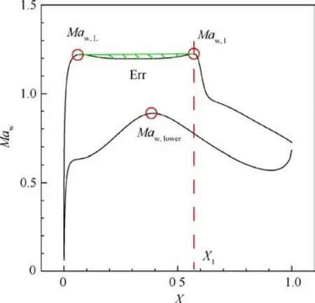
Fig. 11 Definitions of wall Mach number features.

(1) Wall Mach number of the suction peak,Ma:the wall Mach number of the suction peak on the upper surface,which is defined as the largest wall Mach number within the 15% chord length near the leading edge.

(2) Location of the shock wave, X: initially, the shock wave is roughly located by the largest -dMa/dX location ～X on the upper surface. Then, the largest-dMa/dXlocation is found in front of ～X as X.For practical use, the local wall Mach number of Xshould be greater than 1, and the largest -dMa/dX must exceed a specific predefined criterion. Otherwise,it is not a shock wave at this candidate Xlocation.The criterion is related to the number of grid points on the upper surface and the free-stream Mach number,which is - 1.0 in this paper. The more grid points there are on the airfoil surface, the smaller the criterion is.

(3) Wall Mach number in front of the shock wave, Ma:Maof location X.

(4) Highest wall Mach number on the lower surface,Ma.

(5) Smoothness of the suction plateau,Err:the smoothness function of the suction plateau is defined as the area of the shaded region between the suction peak and shock wave. It is used to avoid airfoils on which the suction plateau has a severe pit or fluctuation. The smoothness function can be defined for both the wall Mach number distribution and the pressure coefficient distribution(C).The smoothness of the pressure coefficient distribution is used in the present paper.

3.3. Airfoil sampling of geometry parameters

When generating the airfoil samples, the input vector x is the geometry parameterization parameter,i.e.,the 14 CST parameters. The output vector y obtained by CFD evaluations of x contains flow features to be studied, e.g., the wall Mach number in front of the shock wave(Ma)and shock wave location(X). The other wall Mach number features (Err, Ma,Ma, etc) are used for constraints. The vector Y in Fig. 1 contains performance coefficients that are important in aerodynamic designs, such as the drag coefficient (C) or drag divergence Mach number (Ma).

Supercritical airfoils are transonic airfoils that have several typical features;therefore,airfoil sampling must be carried out under constraints. The constraints utilized in this paper are shown by

s.t. round leading edge, single shock wave,

which specifies that supercritical airfoils have a single shock wave. The fluctuation of the suction plateau (Err) is also kept relatively small,in order to avoid undesirable dent on the suction plateau, which may form an additional shock wave at lower Maand cause larger drag.The constraint of the highest wall Mach number on the lower surface (Ma) avoids the supersonic region on the lower surface when the free stream Mach number is increased,which is a common requirement in industry.The constraint of Manot being too large is to focus the study on practical supercritical airfoils, since the cruise efficiency and off-design performances will deteriorate when the shock wave is too strong. Therefore, the constraints guarantee that the airfoil samples are reasonable for aircraft design, which makes the statistical results applicable for practical scenarios.

The sampling process is conducted under cruise conditions,of which the free-stream Mach number Ma=0.76 and Reynolds number Re=5×10are based on a chord length of 1.0.The flight angle of attack is automatically adjusted in CFL3D by keeping a fixed lift coefficient of C= 0.70.results, and the second row shows the number of airfoils that meet the constraints in Eq. (19).

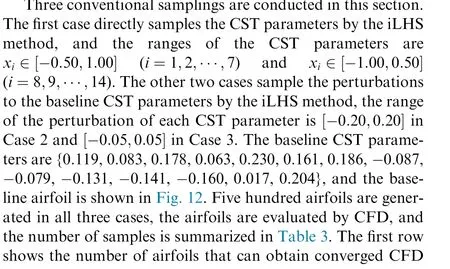
Fig. 12 Baseline airfoil.

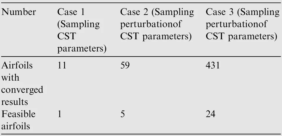
Table 3 Test functions and specified distributions.

Some typical airfoils from the three cases are plotted in Figs. 13-15. Fig. 13 and the results in Table 3 show that directly sampling CST parameters (Case 1) is almost impossible to generate airfoils that have converged CFD simulation,not to mention meeting the constraints in Eq. (19). Although in Cases 2 and 3,sampling the perturbation of CST parameters can increase the ratio of samples with converged results, the ratio of feasible samples is still low. The airfoil samples generated in Case 2(Fig.14)are still not airfoil-like.By reducing the amplitude of perturbation,Case 3 generates more airfoils with converged results, but only a few of them have supercritical wall Mach number distributions, as shown in Fig. 16.Fig. 17 shows the density distribution of the feasible airfoils of Case 3 in the output space of Maand X.This shows that sampling in the input space cannot control the airfoil distribution in the pressure distribution feature space. Therefore, the OSS method is needed to generate samples for further statistical studies.

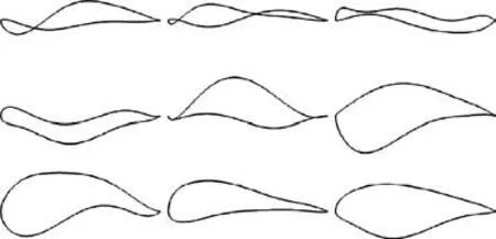
Fig. 13 Airfoils by sampling CST parameters (Case 1).

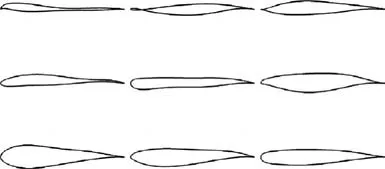
Fig. 14 Airfoils by sampling perturbation of CST parameters(Case 2).

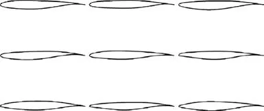
Fig. 15 Airfoils by sampling perturbation of CST parameters(Case 3).

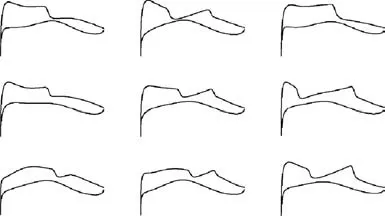
Fig. 16 Wall Mach number distribution of airfoils in Fig. 15.

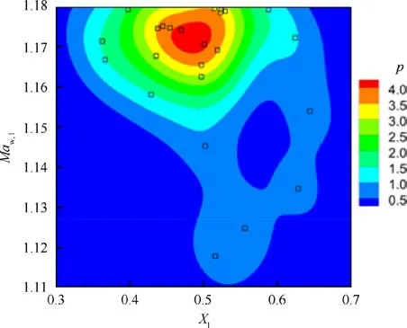
Fig. 17 Density distribution in output space of X1 and Maw，1(Case 3).

3.4. Airfoil sampling of shock wave locations

To study the influence of shock wave location on the drag creep and drag divergence characteristics, airfoil samples with shock wave locations evenly distributed on the airfoil upper surface are needed. To minimize the influence of other flow features, the airfoil lower surface is controlled during sampling, i.e., the seven CST parameters of the lower surface are kept within the range of ±0.05 from the baseline airfoil. The airfoils also have the same （t/c ）of 0.095.

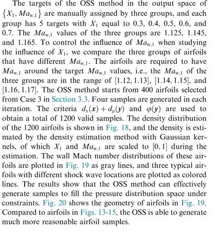
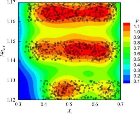
Fig. 18 Density distribution in output space of X1 and Maw，1(sampling airfoil shock wave locations)

3.5. Statistical analysis of airfoil performance

The airfoils are evaluated at several different free stream Mach numbers when the lift coefficient and Reynolds numbers are held the same as those under the cruise condition. The offdesign free stream Mach numbers are 0.700, 0.720, 0.740,0.750, 0.770, 0.775, 0.780, 0.785, and 0.790. The Cvs Macurves of three typical airfoils in Fig. 19 are plotted in Fig.21,which shows that the shock wave location and suction peak have a significant influence on the drag divergence and drag creep. The influence of Xon the Cvs Macurves can vary based on the shock wave strength,which is more significant when the shock wave is stronger, e.g., the difference among the three curves is larger in Fig. 21 (c) than in Fig. 21(a).The influence of Xis larger when the shock wave is more upstream,e.g.,the difference in the Cvs Macurves is larger between airfoils 1 and 2 than between airfoils 2 and 3.To further reveal the influence of these flow features, the drag divergence Mach number and drag increase describing drag creep are studied with different values of flow features.

Fig. 19 Wall Mach number distribution of valid airfoil samples and typical airfoils.

Fig. 20 Geometry of valid airfoil samples and typical airfoils.

Fig. 21 Drag vs Mach number curves of typical airfoils.

Fig. 22 Influence of critical slope k on the X1 vs Ma∞，DD relationship.

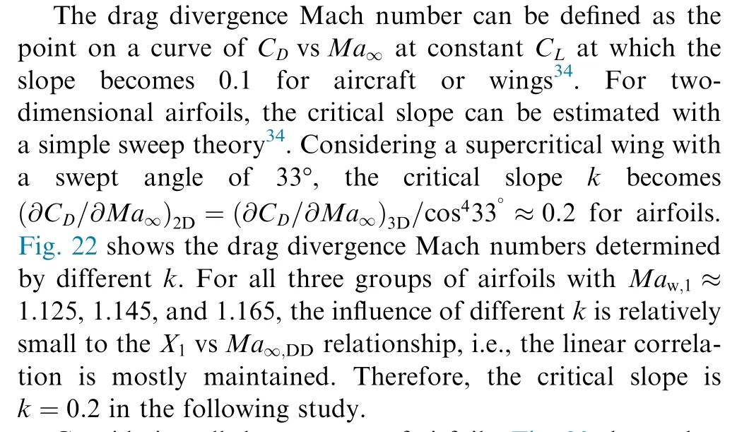
Considering all three groups of airfoils, Fig. 23 shows that Mahas a negative linear correlation with shock wave location X, of which the R-squared (R) value is 0.932.Because all these airfoils share the same lift coefficient and maximum relative thickness, the difference in Maindicates the influence of the pressure distribution features on the technology level factor κ. Therefore, the technology level factor can be described by

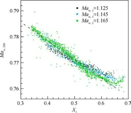
Fig. 23 Linear regression of Ma∞，DD to X1

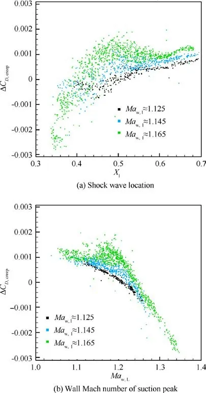
Fig. 24 Influence of flow features on drag creep characteristic.

In contrast, the drag creep characteristics of the airfoils do not have a linear relationship with Xor Ma.Fig.24 shows the influence of Xand Maon the drag creep characteristic,which is represented by the drag coefficient increment between Ma= 0.76 and 0.70, i.e., ΔC=C-C. Although a simple regression is not easy to achieve, Fig. 24 (b) indicates that the drag coefficient rapidly grows when the Mavalues of the airfoils are too high.Therefore, to avoid bad drag creep characteristics, an airfoil should have its Malower than 1.25.

4. Conclusions

The output-space sampling method is an important tool for statistical aerodynamics research on the relationship between flow features and performance. As part of this method, a statistical distance measure of the sample density distribution to the specified distribution is developed. The space-filling property as well as the boundary exploration capability is enhanced by the OSS method. The OSS method is proven to be able to generate samples according to a specified distribution in the output space, and it can achieve a higher proportion of valid samples in all the generated samples than conventional sampling methods.

The output space sampling method is used to generate airfoils with various pressure distribution features. This method is able to efficiently obtain samples according to specified distributions under different constraints.This property further guarantees the accuracy and generality of the statistical research.

Supercritical airfoils generated by the OSS method are statistically analyzed. The results show that the drag divergence Mach number increases when the shock wave is more upstream. Korn’s equation is found to be further expressed as Ma+0.1C+ （t/c ）+0.065X=0.97. The drag creep characteristic deteriorates when the suction peak is greater than Ma=1.25. These relations and constraints can guide the selection of the shock wave location during the process of aerodynamic optimization and design. Furthermore, the quantitative correlations, e.g., the correlation found in this paper and the correlation between shock induced separation and aircraft transonic buffet onset, can significantly reduce computational costs in optimization, because these off-design performance can be estimated by one CFD calculation rather than a series of calculations.

The authors declare that they have no known competing financial interests or personal relationships that could have appeared to influence the work reported in this paper.

This work was supported by the National Natural Science Foundation of China (Nos. 91852108 and 11872230).