Ground maneuver for front-wheel drive aircraft via deep reinforcement learning

Hao ZHANG, Zongxia JIAO, Yaoxing SHANG, Xiaochao LIU,Pengyuan QI, Shuai WU,d

a School of Automation Science and Electrical Engineering, Beihang University, Beijing 100083, China

b Research Institute for Frontier Science, Beihang University, Beijing 100083, China

c Science and Technology on Aircraft Control Laboratory, Beihang University, Beijing 100083, China

d Key Laboratory of Advanced Aircraft Systems (Beihang University), Ministry of Industry and Information Technology,Beijing 100083, China

e Ningbo Institute of Technology, Beihang University, Ningbo 315800, China

f The State Key Laboratory of Fluid Power and Mechatronic Systems, Zhejiang University, Hangzhou 310027, China

KEYWORDS Front-wheel drive aircraft;Ground maneuver;Nose wheel steering;Tire model;Magic equation;Deep reinforcement learning

Abstract The maneuvering time on the ground accounts for 10%–30% of their flight time,and it always exceeds 50%for short-haul aircraft when the ground traffic is congested.Aircraft also contribute significantly to emissions,fuel burn,and noise when taxiing on the ground at airports.There is an urgent need to reduce aircraft taxiing time on the ground.However,it is too expensive for airports and aircraft carriers to build and maintain more runways, and it is space-limited to tow the aircraft fast using tractors. Autonomous drive capability is currently the best solution for aircraft,which can save the maneuver time for aircraft. An idea is proposed that the wheels are driven by APU-powered (auxiliary power unit) motors, APU is working on its efficient point; consequently,the emissions,fuel burn,and noise will be reduced significantly.For Front-wheel drive aircraft,the front wheel must provide longitudinal force to tow the plane forward and lateral force to help the aircraft make a turn. Forward traction effects the aircraft’s maximum turning ability, which is difficult to be modeled to guide the controller design.Deep reinforcement learning provides a powerful tool to help us design controllers for black-box models; however, the models of related works are always simplified,fixed,or not easily modified,but that is what we care about most.Only with complex models can the trained controller be intelligent. High-fidelity models that can easily modified are necessary for aircraft ground maneuver controller design.This paper focuses on the maneuvering problem of front-wheel drive aircraft, a high-fidelity aircraft taxiing dynamic model is established, including the 6-DOF airframe, landing gears, and nonlinear tire force model. A deep reinforcement learning based controller was designed to improve the maneuver performance of front-wheel drive aircraft. It is proved that in some conditions, the DRL based controller outperformed conventional look-ahead controllers.

1. Introduction

The maneuvering time on the ground accounts for 10%–30%of the total operating time,whether it is military or civilian aircraft,1which can not be ignored and should be better used. If the maneuvering time can be reduced, it will benefit a lot. For military aircraft, they can only combat effectively in the sky.Time is life; it is necessary to save all non-combat time, especially the time that when the aircraft taxiing on the ground;For civil aircraft, time is money; airlines can be more profitable, passengers can save flight time, and their travel experience can be improved if the ground maneuvering time can be saved.2–4

Another fact aggravated this situation,that is the operating space is always limited. Most of the airports have only one runway for aircrafts taking-off and landing; only small numbers of airports have two or more runways, followed by high maintenance costs. Solving the queuing problem to improve the efficiency may be a better choice rather than building another runway. Moreover, for the navy, the aircraft carrier’s combat effectiveness depends on the carrier-based aircraft,and the upper limit is not the number of the aircraft, but the inefficient dispatch rate. That is because the deck is space-limited,and aircraft taxiing relies on the tractor operation before take off and after landing, most aircraft are stored in hangars as a result,the cabins are too narrow and time-consuming for tractors to tow the aircrafts out.5,6

Researchers have been making efforts to let the aircrafts taxi autonomously by powered wheels, this approach can increase the maneuver efficiency significantly.Two representative companies named ”WheelTug” and ”Safran” developed products named ”WheelTug” and ”EGTS (Electric Green Taxiing System),” respectively.7,8”EGTS” prefers to drive the aircraft by main wheels,while”WheelTug”prefers the nose wheel.The feasibility of these two solutions have been proved,but it is still a problem that how to drive the aircraft more effectively by powered wheels.

The dynamics of those aircrafts without powered wheels have been investigated a lot.9,10This article focus on the front-wheel-drive aircraft configuration which is more complicated.

For the front drive wheels,only does it maximum its capacity in both longitudinal and lateral directions, can the maneuvering efficiency of aircraft be optimized.10,11Considering the contact force’s black box features between the tire and the runway, a deep reinforcement learning method is introduced into the controller design section to explore a better control performance.

The 6-DOF(Degree of Freedom)model is highly nonlinear,and it is extremely difficult to derive the control law directly;researchers usually design controllers by linearizing models first. However, simplified models mean simple controller, it may ignores many critical features in specific circumstances.12–14

Using DRL (Deep Reinforcement Learning) method,researchers can develop controllers for equipments, games,and other scenarios by training in simulations.12,15–17However,the models used in many related DRL studies are simplified or have parameters that are not easily to be modified,hence the advantages of DRL underutilized. The more complex the model is, the more agent can learn from the environment, and the better the controller works. We are aiming to train an aircraft ground maneuver controller with complex but easily-modified dynamic models using DRL approach,and make the controllers get superior performance in all circumstances.

The outline of this article is organized as follows: In Section 2, the training environments are modeled, where the aircraft dynamic equations are formulated; in Section 3, the dynamics of the aircraft and the wheels are represented as Markov decision process. Besides, the reward and penalty functions are designed; Section 4 gives depictions of the controller schematic diagram and how the network parameters updated; in Section 5, series of simulations are carried out to demonstrate the feasibility of the DRL based control method,followed by discussions; Finally, conclusions are given in Section 6.

2. Ground maneuver training environment

This section gives a detailed description of the training environment modeling. To make the DRL based controller more robust to disturbances and adapt to a wide range of working conditions, a high-fidelity aircraft dynamic model has been established before the controller is trained.

2.1. Aircraft modeling

The study object is the aircraft with front three-point landing gears, F-16 fighter ‘‘Falcon” was chosen for the modeling,shown in Fig.1,followed by details of the dynamics modeling.

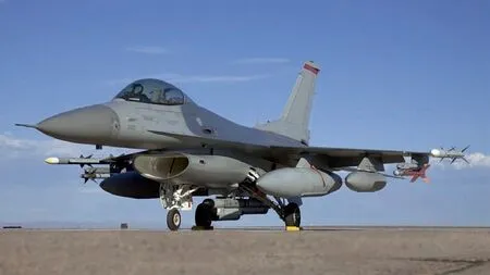
Fig. 1 Illustration of F-16 Fighter.

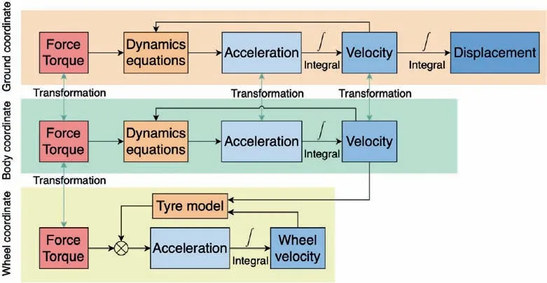
Fig. 2 Schematic of modeling.

To better describe the state variables,three coordinates are introduced to help the modeling: ground coordinate, body coordinate,and wheel coordinates.The specific modeling schematic diagram is shown in Fig. 2.

The transformation method between coordinates is introduced to describe the dynamics for different objects, such as airframe, wheels, etc. Derivatives of variables are integrated to calculate corresponding variables in each coordinate.

2.1.1. Coordinate transformation

The relationship between ground coordinate and aircraft body coordinate is shown in Fig. 3. Where the superscripts indicate which coordinate state variables are in. And Euler angles are used to depict aircraft orientations, the transformation order is yaw, pitch, and roll.

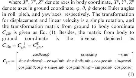
It should be noted that the integral for angular velocities between coordinates are nonlinear and different from that for displacement and linear velocities. The transformation matrix is given in Eq. (2)

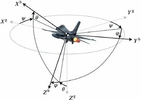
Fig. 3 Relationships among coordinates.

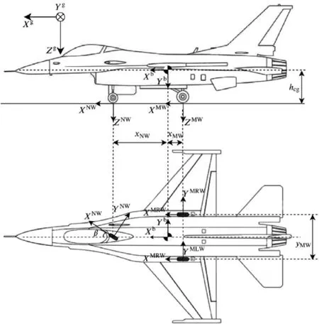
Fig. 4 Wheel coordinates and geometry parameters.

The wheel coordinate is used for wheel dynamics modeling,and the relationship with body coordinate is depicted in Fig.4,where related geometry parameters are denoted. The orientation of main wheels coordinates is consistent with that of body coordinate,and the steering angle should be considered for the nose wheel.

(XNW;YNW;ZNW);(XMLW;YMLW;ZMLW);(XMRW;YMRW;ZMRW)denote the wheel coordinates of each wheel, xNW;xMWdenote the distance in Xbaxis from C.G.(Center of Gravity) to nose wheel and main wheels, hcgis the height of C.G. from the ground, yMWis the wheel span between two main landing gears.

The transformation matrix for force vector from the nose wheel coordinate to body coordinate is given as

where the variable β is the steering angle of front wheel along Zbaxis in the aircraft body coordinate.

2.1.2. 6-DOF airframe dynamics

A 6-DOF dynamic equations of the airframe are established,before which an assumption is presented that the flexibility of the airframe is neglected, hence the airframe can be treated as a rigid body with lumped-mass.18,19

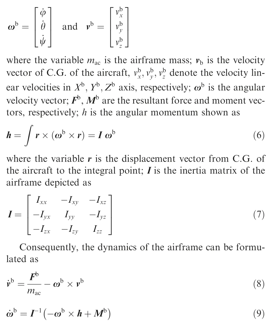
The differential equations of linear and angular momentum of the airframe can be formulated as20

2.1.3. Landing gear dynamics

Different from the cruise phase, the force is mainly from the ground during the taxiing procedure. The dynamic models of landing gears are formulated in this subsection.

Considering the pitch and roll angles are small,the dynamics in longitudinal and lateral directions are neglected, only vertical dynamics are formulated, the vertical landing gear model is shown in Fig.5,where the airframe and the unsprung mass are considered as two separate objects.

The vertical landing gears dynamic equations are formulated as

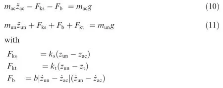
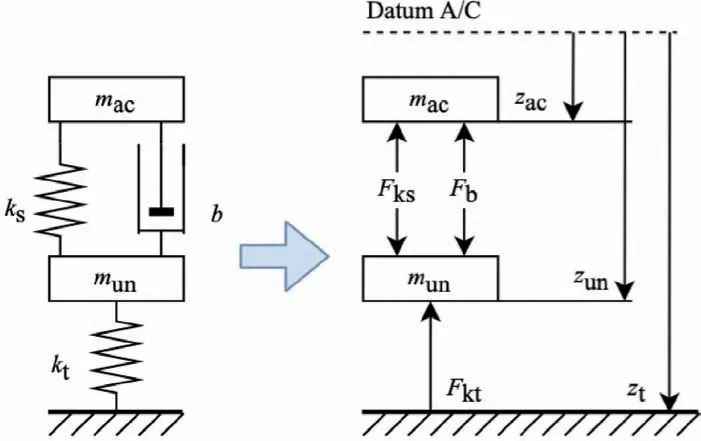
Fig. 5 Schematic of single landing gear model.

where munis the unsprung mass, g is the gravity factor, the variable, ¨zac, zun, ztare the positions of C.G. of aircraft, the unsprung mass, and the tire along Zbaxis, respectively.Fks,Fb, Fktare the supporting force from the return spring of the shock absorber, the damping force, and the supporting force of the elastic tires, respectively. ksis the coefficient of return spring,ktis the stiffness coefficient of the tire,b is the damping coefficient of the shock absorber.

It should be noted that the damping force is not proportional to the unsprung mass velocity but to the square of it because of hydraulic resistance oil. Moreover, the continuity equation for resistance fluid is given in Eq. (12), where the damping force Fbis derived from using equation Fb=ΔPAp.

where the variable q is the flow rate of resistance oil in the shock absorber, Apis the shock absorber piston area, Cdis the flow coefficient of the resistance orifice,A is the orifice flow area,ρ is the oil density,ΔP is the pressure difference between the two chambers of the shock absorber. Hence, the damping ratio b is derived as

The multi-LG dynamic models can be formulated similarly,the schematic diagram is depicted in Fig.6.zNW;zmNW;ztNWare the positions of the attachment point of nose landing gear,the unsprung mass of nose landing gear mover, the contact point of nose wheel on the ground in Z axis, respectively,ksNW;cNW;ktNWare the coefficient of return spring, the damping coefficient of shock absorber,the tire stiffness coefficient of nose wheel, respectively, mNWis the unsprung mass of nose landing gear,similarly,the subscript MW denote those of main landing gears. zCGis the position of C.G. in Z axis.

The only difference is that the mass on the return spring is omitted; force interfaces are used to get the airframe 6-DOF model and landing gear models connected.

2.1.4. Wheel dynamics modeling

The dynamic models of wheels are highly nonlinear,the model is established in two directions in wheel coordinates.

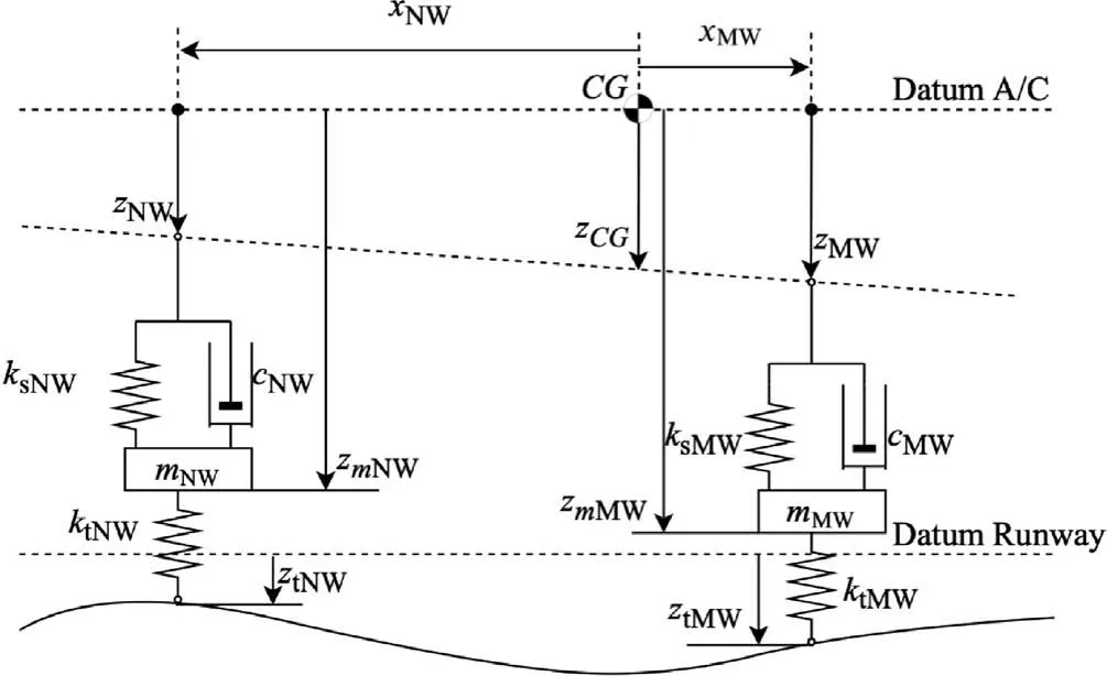
Fig. 6 Schematic of multi-LG model.

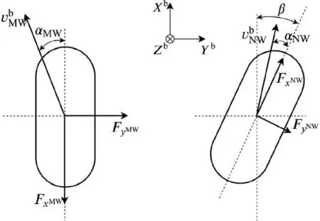
Fig. 7 Illustration of target path transition.

where the variable vxw, vyw, vxb, vxbare the wheel center velocity, whose subscripts denote the coordinate. The detailed geometry relationship is shown in Fig. 7.

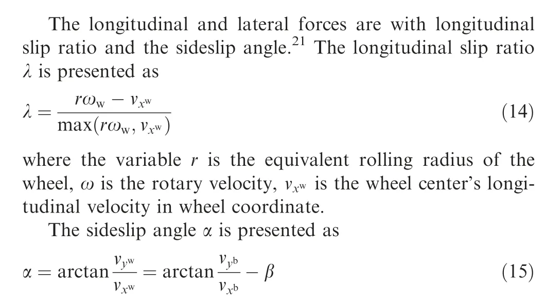
The longitudinal and the lateral friction forces under specific vertical load can be formulated with one equation as21

where the variable x is slip ratio λ for the condition with only longitudinal slip, and it is sideslip angle a for that condition with only lateral slip.

Combining the longitudinal and lateral forces together,the friction forces are derived as

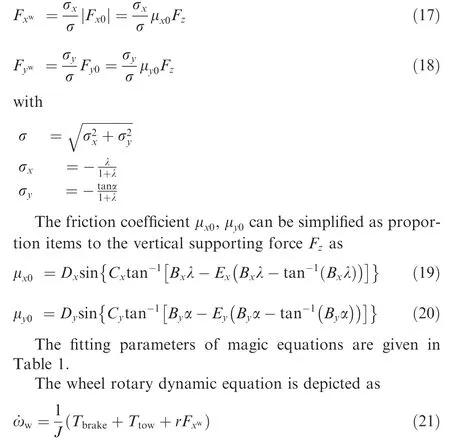
Table 1 Magic equations parameters.

where J is the wheel mover inertia,Tbrakeis the braking torque,Ttowis the towing torque produced by the nose wheel motor.The torque from the landing gears is depicted as

where LLGis the displacement vector from C.G. of aircraft to the contact point of landing gear wheels.

2.1.5. Aerodynamic force modeling

The air load of the aircraft is also simplified to a lumpedparameter model,22,23depicted as

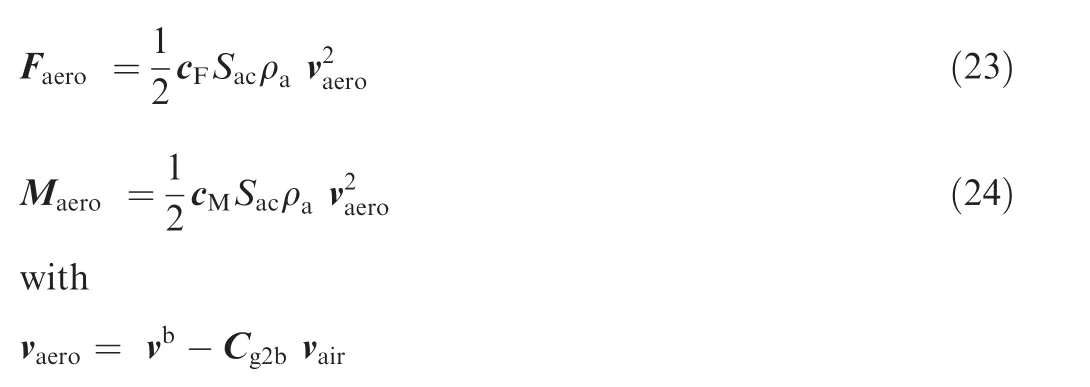
Where Faeroand Maeroare the aerodynamic force and torque vectors, respectively, cFand cMare the coefficients matrix,Sacis equivalent area, ρais air density, vaeroare the relative velocity between the aircraft and the air, vairis the airspeed in ground coordinate.

2.1.6. Aircraft parameters

The parameters of the airframe,24,25landing gears,wheels used in the training environment modeling are given in Table 2.

3. Markov decision process modeling

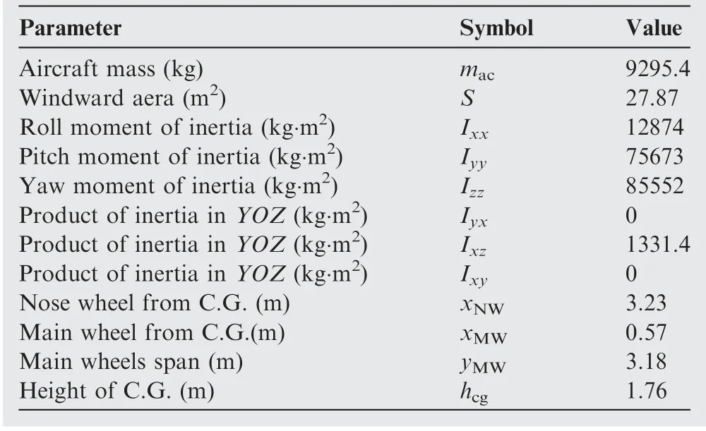
Table 2 Parameters of the F-16 falcon.

describes the action space; Psais a state transition probability matrix for taking action a in state s; R is the reward (penalty)function guiding the controller in learning and it should be designed carefully; the return G is the total reward of an episode.

3.1. Aircraft ground maneuvering state space

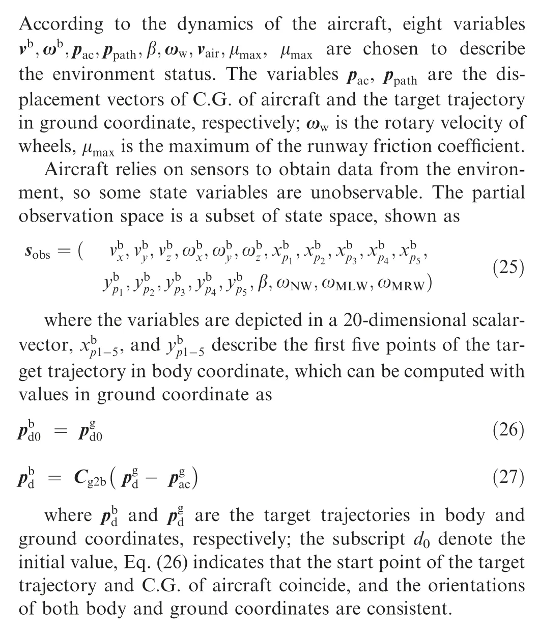
3.2. Aircraft ground maneuvering action space

For the aircraft ground taxiing configuration proposed in this paper, the aircraft can move forward by wheels and make a turn by steering the nose wheel. As a result, the action space can be presented using a two-tuple as

where TNWis the towing torque of nose wheel motor, the maximum of which is limited by the runway friction force.

3.3. Reward function design

The principle of RL is to make the agent learn to obtain as much rewards as possible during the agent’s life time. The reward function needs to be carefully designed to avoid the situation that the RL agent would obtain a higher score instead of completing the task with wrong reward function.

The objective is to train an intelligent agent to improve aircraft mobility on the ground. The aircraft tends to move and turn at a high velocity to gain more rewards in a limited time.It should also keep a high trajectory tracking accuracy simultaneously. The reward function is designed in four parts:rewards for higher velocity Rvel, for higher tracking accuracy Racc,for closer distance to the next checkpoint Rd,and the penalty for wheel slip Rslip.

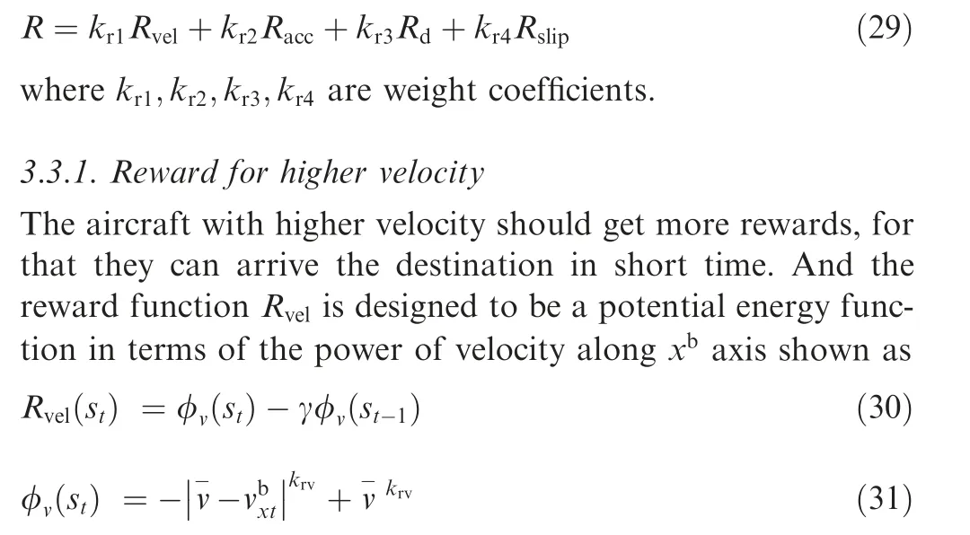
where γ is the time discount factor, φv(st) is the potential energy function, v- is the threshold of maximum taxiing velocity, krvis the coefficient of the exponent.

3.3.2. Reward for higher tracking accuracy

The optimal controller should keep the aircraft taxiing along the target trajectory, so the optimal tracking errors along ybaxis should be zero; any non-zero value should be penalized.As a result, the tracking accuracy reward is designed to be a power function of yb, shown as

3.3.3. Reward for closer distance

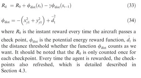
The most important thing is that we should guarantee that our agent can pass every checkpoint along the target trajectory without a missing;the distance reward is designed in two parts:an instant reward for arriving at every checkpoint and a trend reward in terms of a potential energy function of the distance from next checkpoint.

3.3.4. Penalty for wheel slip

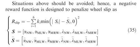
Wheels may slip when aircraft make a sharp turn at a high longitudinal velocity,and then make aircraft out of control.That is because of the non-linear and bounded tire friction characteristics. The driving wheel will exceed the speed threshold in a short time when the towing torque is too large, then wheels slip and the contact force reduced. The aircraft then moved into an unstable zone and deviated from the desired trajectory as a result.26–28

where kiis the weight factor,a and λ are threshold values to let slip reward be only negative when it exceeds the threshold.

3.3.5. Discount factor and value function

Considering that the current reward is more critical than that faraway, discount factor γ is introduced to penalize the future rewards with higher uncertainty. Using the iteration approach,the state value function and the state-action value function are depicted as

3.3.6. Reward termination

The mission fails when aircraft deviates from the target trajectory and never return even though the longitudinal velocity is high. Hence, all the aircraft dynamics parameters are restricted, shown as

The episode will be reset to prevent above situations if the aircraft leaves the trajectory too far or exceeds the state variable constraints. Furthermore, the episode job will be done if the aircraft reaches the endpoint.

4. Reinforcement learning training scenario

The detailed DRL training scenario is constructed in this section, followed by tricks to optimize the DRL network performance, and the target trajectory generation method is given.

4.1. RL framework

The DRL framework used in this paper is PPO2 (Proximal Policy Optimization),29,30the schematic diagram of which is presented in Fig. 8.

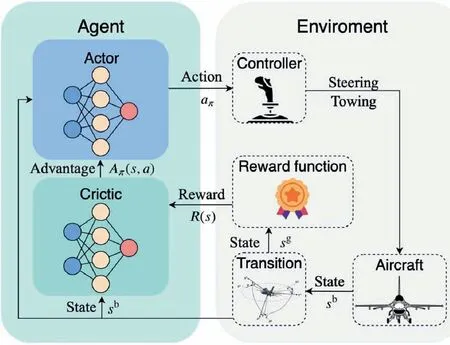
Fig. 8 Schematic diagram of RL training.

The environment refreshes state st+1according to the action atand returns reward rtderived from st. The agent observes the state sampled from the environment, then get rewards when trying different actions. It finally learns to get as much rewards as possible to complete the task as we want.

The DRL agent consists of two neural networks:actor and critic, both of which can handle continuous state and action spaces. The objective is to train an actor network to learn the parameters θ of the policy πθ,and the actor can map the observation sobsto action aπ.aπis the optimal action choice in current state s.The critic is responsible for update the actor policy using advantage value derived from sband reward R(s). This approach could guide the actor in finding the best policy π*.

The transition module is responsible for transforming the state variables between coordinates and sampling partial observation variables from states.

4.2. Network parameters update method

The RL network optimizes the action selection policy by a trial-and-error process in the simulated environment.The policy network parameters are critical to the agent, and how the parameters are updated is depicted in Fig. 9.

AC network integrates the advantages of both value-based and policy-based RL.31For the critic network, the output is the state-action value approximated with parameter w shown as

To reduce the gradient bias, a baseline function Vπθ(s) is introduced which is independent from the policy π,and would not change the expectation of the objective function. It normalizes Q(s;a) value to the value baseline V(s), improving the learning efficiency and stability.

Hence, the advantage function is designed as

According to Bellman equation,33TD-error δ is an unbiased estimation of the advantage function. Hence, we use one neural network to compute the approximate advantage value, in this way, we use only one set of parameters to estimate the state value. Hence the computational complexity is reduced. The policy gradient becomes

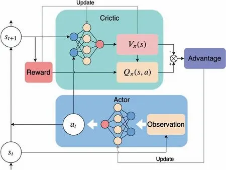
Fig. 9 Schematic diagram of RL agent.

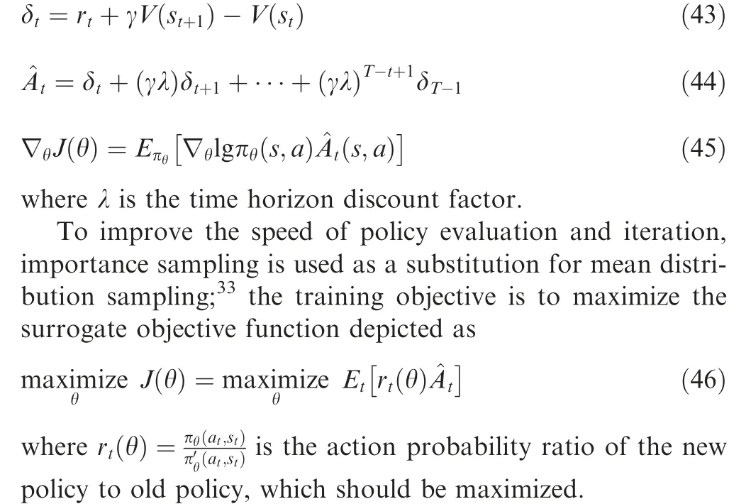
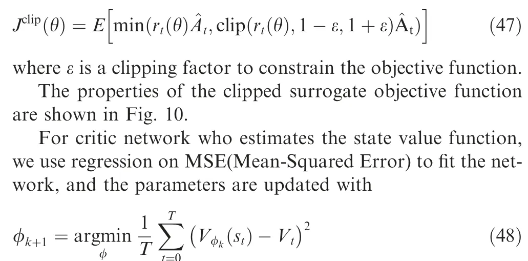
It should be noted that an assumption has been made that the action distribution of the two policies are considered consistent,which means excessively parameter update may lead to a large distribution variance, then the stability of the policy update will be affected.

To avoid this from happening, we slow down the stride of the policy parameter update. The surrogate objective function is clipped as29

The input state variables are normalized to a ∊[-1;1] distribution to improve the neural network’s convergence speed.

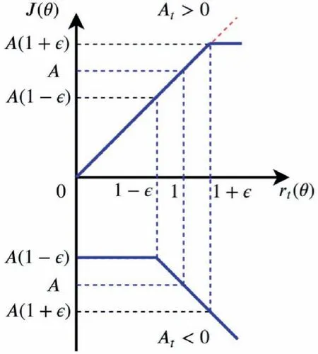
Fig. 10 Surrogate objective function.

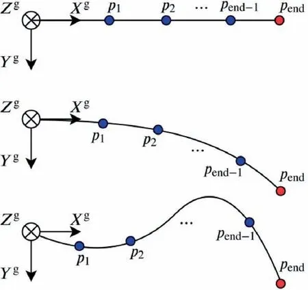
Fig. 11 Target trajectories illustration.

4.3. Target trajectory

The simulation starts with random initialization. Both target trajectories and initial dynamics values are set randomly to make our trained agent explore more state and action spaces and be more robust to disturbances. Three typical trajectories are shown in Fig. 11.

The target trajectory is depicted as a series of points[(xp1;yp1);(xp2;yp2)∙∙∙(xpend;ypend)] in the ground coordinate,only the next five points are selected and transformed into body coordinate to meet the agent observation needs.The trajectory transformation between coordinates is depicted in Fig. 12.

Each time the aircraft passes a point, the trajectory sequence refreshes, the first point is erased from the trajectory sequence, then the remaining points move forward. The agent observes the first five points as its input.Eq.(49)represents the criterion whether the aircraft passes the trajectory point p1.

5. Experimental studies

In this section,the training method is given;the pseudocode is presented, followed by the training results and discussions.

5.1. Training method

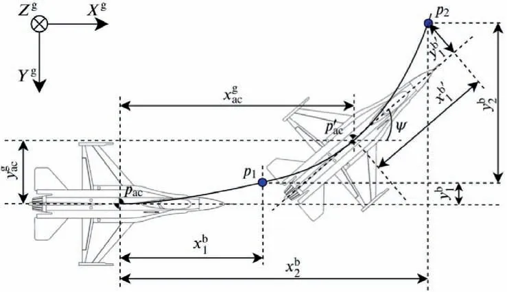
Fig. 12 Illustration of target trajectory transition.

It takes many iterations to converge the network in the training process.In each iteration,actors run policy π(θk)to generate experience trajectory data, with advantage values computed. Then mini-batch gradient descent method is used to fit the critic network, and the actor network is trained using PPO.

To balance the numerical accuracy and the rewards obtaining stability in the simulation,the temporal resolution is set to be 0.05 s, the model updates at 20 Hz. The maximum time steps of each episode is 1000.

Pseudocode

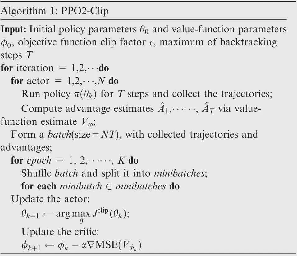
Algorithm 1: PPO2-Clip Input:Initial policy parameters θ0 and value-function parameters φ0, objective function clip factor ∊, maximum of backtracking steps T for iteration = 1,2,∙∙∙do for actor = 1,2,∙∙∙,N do Run policy π(θk) for T steps and collect the trajectories;Compute advantage estimates ^A1,∙∙∙∙∙∙, ^AT via valuefunction estimate Vφ;Form a batch(size=NT), with collected trajectories and advantages;for epoch = 1, 2,∙∙∙∙∙∙, K do Shuffle batch and split it into minibatches;for each minibatch ∊minibatches do Update the actor:θk+1 ←arg max θ Jclip(θk);Update the critic:φk+1 ←φk-a∇MSE(Vφk)

5.2. Results and discussions

The DRL agent has been trained online for over 600 k time steps,the total rewards of an episode during the training procedure is shown in Fig.13,where we can find the current AC network outperforms the past during the training,and finally got a total of about 1500 rewards after 500 k training time steps.

Testing results of three trajectory examples of Fig. 11 are shown in Figs. 14–16.

Fig. 14(a) shows the target and actual trajectory 1, where we can see the agent trained for 500 k time steps (trained agent) outperforms the agent trained for 100 k time steps(training agent) during the 1000 time steps(50 s). The trained agent has less tracking errors. It accelerates to the maximum velocity earlier shown in Fig.14(b). The accelerator and steering angle of action spaces are depicted in Fig. 14(c) and (d),where we can see the action variance drops down significantly,which means the actor-network converged.

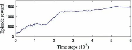
Fig. 13 Total rewards in raining (smoothed).

Fig. 14(e) presents the rewards of the two agents; In this simple target trajectory,the training agent is underperforming;it only gets about half of the optimal rewards. In the meantime, the trained agent gets close to the optimal reward as the red solid line shows. The reward for higher velocity and reward for closer distance of the training agent are much smaller than those of the trained agent. For trained agent, the reward for tracking accuracy, and the penalty for wheel slip are large negative values, which eliminate the positive reward and lowers the total rewards.

Fig. 15 shows the testing results in trajectory 2, the trained agent has a better performance; the training agent only passes about 150 meters during 1000 time steps.Both agents get fewer rewards in this single turn trajectory scenario than that in trajectory 1.

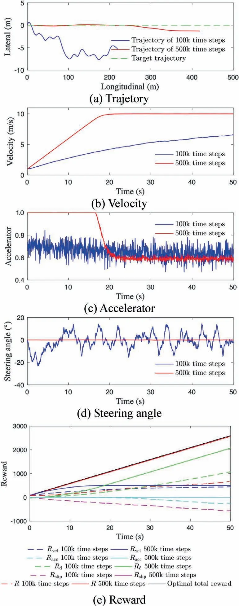
Fig. 14 Testing results of trajectory 1.

We also compared the performance of two different controllers: DRL based controller and Look-ahead (LA) controller;34–37The DRL controller is trained for 500 k time steps.The total reward of the LA controller is computed using the same reward and penalty functions. We can see that the DRL based controller performs as well as the conventional LA lateral controller shown in Fig. 16(a), and even a little better in sharp turn scenarios shown in Fig. 16(b). The LA controller performs better at first and is overtaken later in the sharp turn section. That is because the DRL based agent can lower the speed according to the current state variables and upcoming trajectory curvature to prevent the aircraft from lateral instability caused by tire skidding and then large tracking errors are avoided.

From the three classical trajectory examples,it was demonstrated that DRL based controller have pretty performance after a certain period of training,and further enhance the performance of aircraft ground taxiing control.

6. Conclusions

Using DRL approach proposed in this paper, we can quickly design a controller for aircraft ground taxiing control. The DRL-based controller can follow the target trajectory to reach the destination as quickly as possible and not deviate from the trajectory.

With high-fidelity aircraft taxiing dynamic models and detailed training scenario design, the feasibility of DRL based controller for aircraft taxiing control is demonstrated in this study,this article provides an overview of how the use of data for aircraft maneuvering can be realized in the future.

Declaration of Competing Interest

The authors declare that they have no known competing financial interests or personal relationships that could have appeared to influence the work reported in this paper.

Acknowledgements

Funded by National Natural Science Foundation of China(No. 51775014), Open Foundation of the State Key Laboratory of Fluid Power and Mechatronic Systems of China (No.GZKF-202010), National Key R&D Program of China (No.2019YFB2004503), and the Science and Technology on Aircraft Control Laboratory of China.