A physics-based framework for online surface roughness assessment for high-pressure turbines

Jie LIU, Zelig LI, Houman HANACHI

a National Research Base of Intelligent Manufacturing Service, Chongqing Technology and Business University,Chongqing 400067, China

b Department of Mechanical and Aerospace Engineering, Carleton University, Ottawa, ON K1S 5B6, Canada

c Algonquin College, Ottawa, ON, K2G 1V8, Canada

KEYWORDS Fault inference;Gas turbine;Health monitoring;Operational data;Performance deterioration;Surface roughness;Turbine

Abstract Surface roughness is a critical health parameter of a turbine blade due to its implications on blade surface heat transfer and structural integrity. This paper proposes a physics-based online framework for Gas Turbine Engines(GTE),in order to assess the blade surface roughness in a highpressure turbine without engine shutdown. The framework consolidates Gas Path Analysis (GPA)based performance monitoring models and meanline turbomachinery analysis,using a novel GPAmeanline matching process. This extracts meaningful performance deviation trends from GPA,while addressing the uncertainties associated with the measurements and modelling. To relate efficiency loss to surface roughness severity, a meanline-based system-identification process has been developed to establish the meanline representation of the turbine stage, and to incorporate the empirical surface roughness loss correlations. The roughness loss correlations have been evaluated against recent transonic test data in the literature. A modification to the compressibility correction factor has been made according to the evaluation outcome, which improved loss predictions compared to the experimental measurements. The framework was tested on the three-year operational data of a cogeneration GTE, and the results verified the framework’s potential for online surface roughness monitoring. The predicted surface roughness showed agreement in both trend and the magnitude-level with the measurements reported in the literature.

1. Introduction

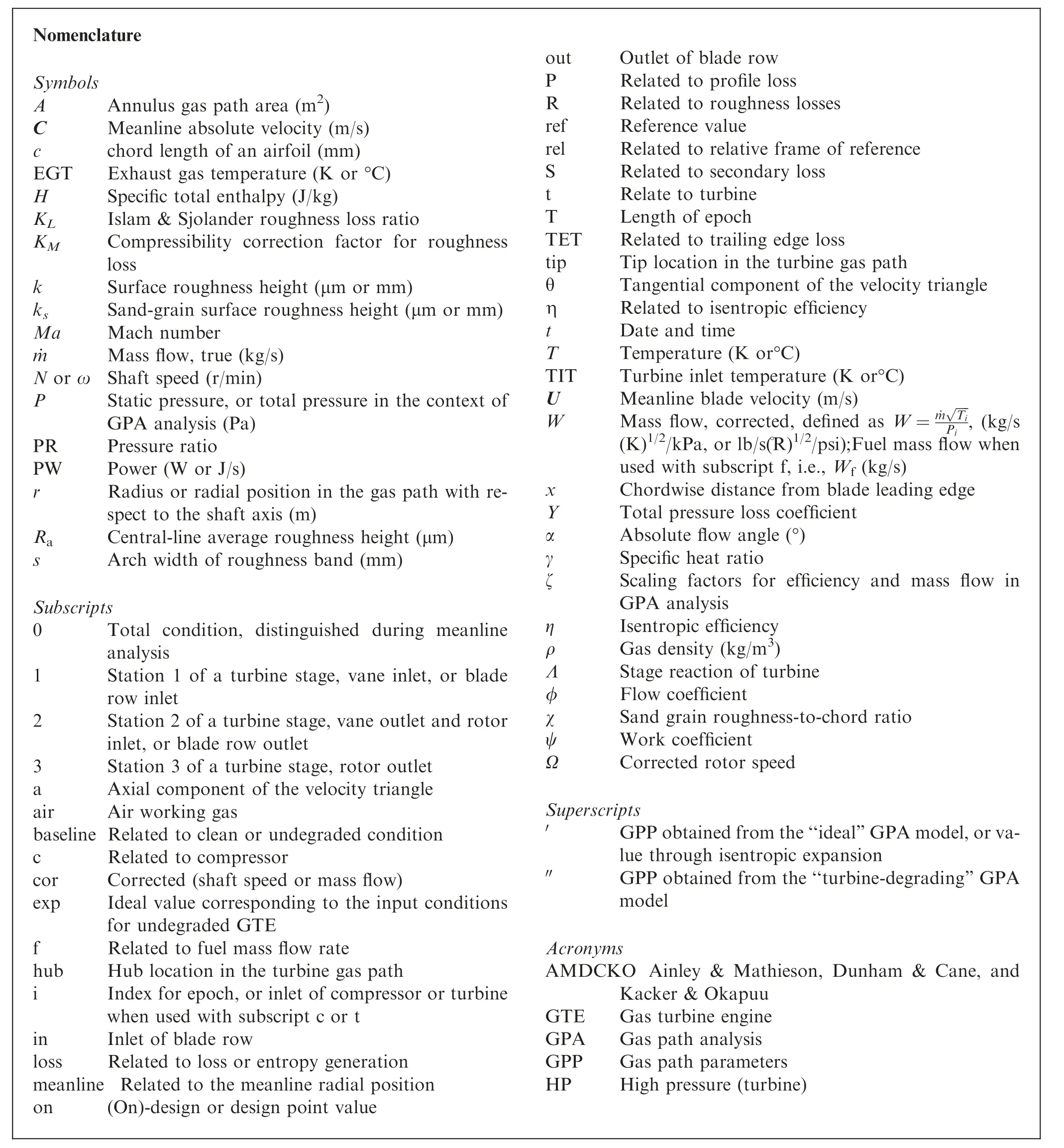
Nomenclature Symbols AAnnulus gas path area (m2)CMeanline absolute velocity (m/s)cchord length of an airfoil (mm)EGTExhaust gas temperature (K or °C)HSpecific total enthalpy (J/kg)KLIslam & Sjolander roughness loss ratio KMCompressibility correction factor for roughness loss kSurface roughness height (μm or mm)ksSand-grain surface roughness height (μm or mm)MaMach number ˙mMass flow, true (kg/s)N or ω Shaft speed (r/min)PStatic pressure, or total pressure in the context of GPA analysis (Pa)PRPressure ratio PWPower (W or J/s)rRadius or radial position in the gas path with respect to the shaft axis (m)RaCentral-line average roughness height (μm)sArch width of roughness band (mm)Subscripts 0Total condition, distinguished during meanline analysis 1Station 1 of a turbine stage, vane inlet, or blade row inlet 2Station 2 of a turbine stage, vane outlet and rotor inlet, or blade row outlet 3Station 3 of a turbine stage, rotor outlet aAxial component of the velocity triangle airAir working gas baseline Related to clean or undegraded condition cRelated to compressor corCorrected (shaft speed or mass flow)expIdeal value corresponding to the input conditions for undegraded GTE fRelated to fuel mass flow rate hubHub location in the turbine gas path iIndex for epoch, or inlet of compressor or turbine when used with subscript c or t inInlet of blade row lossRelated to loss or entropy generation meanline Related to the meanline radial position on(On)-design or design point value?outOutlet of blade row PRelated to profile loss RRelated to roughness losses refReference value relRelated to relative frame of reference SRelated to secondary loss tRelate to turbine TLength of epoch TETRelated to trailing edge loss tipTip location in the turbine gas path θTangential component of the velocity triangle ηRelated to isentropic efficiency tDate and time TTemperature (K or°C)TITTurbine inlet temperature (K or°C)UMeanline blade velocity (m/s)WMass flow, corrected, defined as W=˙m ■■■■Ti Pi , (kg/s(K)1/2/kPa, or lb/s(°R)1/2/psi);Fuel mass flow when used with subscript f, i.e., Wf (kg/s)xChordwise distance from blade leading edge YTotal pressure loss coefficient αAbsolute flow angle (°)γSpecific heat ratio ζScaling factors for efficiency and mass flow in GPA analysis ηIsentropic efficiency ρGas density (kg/m3)ΛStage reaction of turbine φFlow coefficient χSand grain roughness-to-chord ratio ψWork coefficient ΩCorrected rotor speed Superscripts′GPP obtained from the‘‘ideal”GPA model,or value through isentropic expansion′′GPP obtained from the‘‘turbine-degrading”GPA model Acronyms AMDCKO Ainley & Mathieson, Dunham & Cane, and Kacker & Okapuu GTEGas turbine engine GPAGas path analysis GPPGas path parameters HPHigh pressure (turbine)

Gas turbine engines (GTEs) are subjected to various component degradations over the service life, resulting in their gradual performance deterioration. Physical degradations of components, reflected by the changes in the operational parameters,such as power output and exhaust gas temperature(EGT), result in decreased efficiency and changes in flow capacity.1Degradations can be categorized into two types:short-term recoverable degradations and long-term nonrecoverable degradations. Short-term degradations are mainly caused by the compressor fouling. Fouling occurs due to the adhesion of airborne particles on the compressor blades and vanes. Long-term non-recoverable degradations are caused by permanent changes of geometry, corrosion, or removal of materials from the components. For both cases, the development of degradations causes an increase in operational cost,and if not mitigated, could eventually lead to the failure of the components. Diakunchak estimated an excessive annual cost of$522000 for a 46.5 MW GTE,which was assumed with a conservative 3% loss in power and 1% increase in heat rate after 8000 hours of operation, due to unmitigated fouling.2In an extreme case, the combination of compressor blade profile changes and airflow distortions caused by fouling can lead to the aerodynamic stall of later stages, and can trigger surge,resulting in blade damage.3

While compressor wash can recover the short-term performance deterioration due to fouling, the long-term deteriorations are non-recoverable unless the components are repaired or replaced. Common non-recoverable degradations include erosion, corrosion, and the increase of tip-clearance. Positioned directly downstream of the combustor, the High-Pressure (HP) turbine vanes and blades are subjected to surface roughening, due to foreign particle deposition, hot corrosion, erosion, and coating spallation.4The survey by Tarada on used turbine blades from 58 GTEs suggests that turbine blades of longer service life tend to have higher surface roughness.5The surface roughening not only causes additional aerodynamic losses but also increases heat transfer at blade surface, which reduced the life of the blade due to overheating.6Therefore, in addition to causing performance deterioration,surface roughness accelerates the structural deterioration of vanes and blades, and consequently, reduces remaining usable life.

Maintenances are scheduled to mitigate the degradations,recover performance losses and prevent catastrophic failures.Due to the high-costs associated with downtime, the maintenance philosophy has been shifting from preventive maintenance to reliability-centred maintenance with the advancement of GTE diagnostic and prognostic techniques.1Regardless, the fault detection methods (i.e., physics-based,data-driven, or hybrid) mainly reveal performance deviations or fault indications, and are not sufficient to provide further insights on the component-level fault severities,such as surface roughness and tip-clearance. However, the physical implications revealed by the fault severities are essential for understanding the degradation conditions of the critical components, which determines the overhaul schedules. Therefore,to truly attain the cost-saving benefit of reliability-centred maintenance through condition-based downtime scheduling,online assessment of the physical fault severities is crucial.

Although online techniques are available for tip-clearance measurements, such as borescope photography,7to authors’best knowledge, there is no online performance-based monitoring method available in the literature for assessing the surface roughness severity of the turbine blades and vanes,which is usually measured offline.5,8Studies have been conducted to understand the effect of surface roughness on aerodynamic loss and heat transfer, including a series of research programs conducted at authors’institution, Carleton University, including the works by Kind et al.,9Yuan & Kind,10Islam and Jouini et al.11,12These contributions,however,have never been utilized in the area of online condition monitoring. Nevertheless, the observations and the subsequent conceptualizations of the surface roughness loss effects suggest the potential feasibility of assessing turbine surface roughness through performance data.

With these motivations, this paper proposes a novel online monitoring framework, to advance component-level damage assessment using the operational data acquired from basic GTE instrumentation.The framework bridges the gap between GTE performance monitoring techniques and the understanding of the aerodynamics penalty due to surface roughness of turbine blades. The goal of the online framework is to determine the turbine surface roughness condition of a GTE during its operation.

To achieve this goal, the proposed framework integrates both system-level gas path analysis (GPA) and componentspecific turbine meanline analysis.The uncertainties associated with GPA, due to the low sampling rate of the operational data, as well as the modelling assumptions, pose challenges for the extraction of valid information from the results. At the same time, the GPA on turbine degradation is susceptible to compressor fouling effects. A GPA-meanline interfacing process was consequently developed to resolve or alleviate these challenges. A meanline surface roughness identification process was also proposed to establish a meanline model for an existing turbine stage. The process also determines roughness severity using the empirical roughness loss models developed by previous works.

The present work also evaluated the empirical roughness loss models developed by Islam & Sjolander11and Jouini et al.,12before integrating the models into the framework.The evaluation was focused on roughness loss prediction under transonic flow conditions, using the wind tunnel study outcomes of Yuan and Kind.10

The remaining part of the paper is organized as follows.The proposed framework and its key components are described in Section 2. As part of the meanline modelling,the validation and modification of the roughness loss correlation are also presented in the same section.The effectiveness of the proposed online framework is examined in Section 3,through its application to the three-year operational data of a 4MWe cogeneration GTE powerplant. Finally, the conclusions and future works are summarized in Section 4.

2.Physics-based framework for online turbine surface roughness assessment

The current section first briefly presents the GTE and turbine modelling methods adopted by the proposed online turbine surface roughness assessment framework. The system-level gas path analysis for a single-spool GTE is described first,followed by the meanline analysis for axial turbines. The advantages and limitations of both modelling methods for incorporation in the online surface roughness assessment framework are briefly discussed. These limitations motivated the development of the key components of the proposed framework.

The empirical surface roughness loss correlations by Islam11and Jouini et al.,12which are incorporated in the turbine meanline model, are then discussed. The correlations’ability to predict roughness loss under transonic flow condition was evaluated against the wind tunnel results by Yuan and Kind.10This part of the discussion also includes the proposed modification to the roughness loss correlations.

Finally, the main contribution of the present work, an online surface roughness assessment framework for HP turbines, is presented.

2.1. Gas path analysis method

The GPA condition monitoring method utilizes thermodynamic model and measurement data of the GTE to detect and assess the deterioration of various engine modules. The GPA method for GTE condition monitoring was first introduced by Urban13in the 1970s and became well established in the 1980s. The original GPA modelling techniques were based on linear models. Recently, the research interest in GPA analysis has shifted to nonlinear modelling, such as the work of Li14and Larsson et al.,15as well as transient modelling, such as the work of Panov16and Meher-Homji and Bhargava.17The authors’ research group has also developed several nonlinear GPA techniques for single-shaft GTEs,which are capable of capturing both the short-term recoverable compressor fouling,18as well as the long-term non-recoverable degradations in the turbine subsystem.19

GPA utilizes thermodynamic cycle model of a GTE, and the monitored operating conditions to predict the expected performance. An example of GTE cycle model is shown in Eq.(1).

The cycle model requires monitored conditions,which generally include compressor inlet temperature (Tci) and pressure(Pci),relative humidity(π),shaft speed(N),fuel mass flow(Wf)and EGT. The model calculates expected power output corresponding to the operating conditions for the undegraded GTE.The Gas Path Parameters(GPP)are also resolved.As the components of a GTE degrade, the original model deviates from the actual condition of the GTE, and the differences between the predicted power and the measurement grow over time.These differences are captures and quantified for detection of performance deterioration symptoms. For example, Hanachi et al. developed various indicators to detect compressor fouling.20For the convenience of discussion, this approach is referred to as the ‘‘ideal” GPA model.

In an alternative approach,Hanachi et al.resolved the cycle model inversely,in order to monitor the long-term degradation of turbine.19In this ‘‘turbine-degrading” GPA approach, turbine characteristics map is scaled until the model predictions match the measurement values. This in turn, resolves the turbine degradation symptoms over time, namely, changes in its mass flow capacity and isentropic efficiency. Eq. (2) summarizes such a model:

where ζ is the turbine map scaling factor,and the subscripts W,t and η,t indicate turbine mass flow and isentropic efficiency respectively.

From the perspective of GTE condition monitoring, both the ideal and turbine degrading models demonstrated effectiveness in capturing the short-term compressor fouling and longterm turbine performance deterioration, respectively. However,to be used as a part of the component-specific fault severity assessment framework, the following limitations and challenges needs to be addressed:

1. The GPA results usually possess significant amount of noise,due to the measurement uncertainties,the thermodynamic modelling assumptions and numerical errors. While the noise level is tolerable for the purpose of performance monitoring, it can lead to divergence of the solution when applied to the component-specific models, such as the turbine meanline model presented in the subsequent section,which has a higher demand for valid input data.

2. For the same severity level of a fault,such as a specific surface roughness height on the blade surface, the associated efficiency loss can vary dramatically under different operating conditions. While the GPA method does not necessary consider such an effect for mere fault indication purposes,the component-based modelling requires the clear distinction of operating conditions and associated effects, so as to accurately assess the fault severity.

3. In the turbine-degrading model,the short-term compressor fouling effect is usually identified and alleviated by only considering the data within a limited period after each compressor wash,where fouling effect is at minimum.Although Hanachi et al. suggested a five-day sampling period after each wash to alleviate the fouling effect, the value was based on authors’ experience and does not apply to the GTEs operated in different environments.19In reality, the fouling rate is dependent on the environmental conditions as well as the wash quality,which vary over time.A procedure is still required to determine a suitable sampling period, in which the fouling effect is minimum, and the data quantity is sufficient to address the challenges mentioned in (1) and (2).While utilizing both the ideal and the turbine-degrading

GPA models according to inherent strengths, the proposed surface roughness assessment framework attempts to alleviate the aforementioned limitations and challenges associated with the GPA methods through an epoch-based sampling process.This is presented in Section 2.4.

2.2. Meanline turbine aerodynamic modelling

The meanline aerodynamic modelling method is originally a low-fidelity design and performance analysis tool used in the preliminary development phase of a turbomachine.21It determines key turbomachinery parameters prior to more detailed high-fidelity design and analysis. The meanline turbine model uses the flow conditions at the mean radius of the vane or blade,which is assumed to be a valid representation of the flow across the full span. The mean radius is defined as the radius that divides the gas path area in half:

The meanline model is governed by the conservation of mass and the Euler turbine equation (i.e., the conservation of energy) as follows:

where m is mass flow rate,ρ is gas density,A is annulus area of the gas path,ΔH is enthalpy change due to the work of the turbomachine,ω is shaft speed,r is the mean radii,and Caand Cθare the axial and tangential flow velocities respectively. The subscript ‘‘in” and ‘‘out” indicate the inlet and outlet location of the turbine stage respectively. Since, in most cases, the working fluid of a turbine is a compressible ideal gas, the following isentropic relationships between static and total conditions are used:

where γ the specific heat ratio of the working fluid, i.e., combusted gas,M is Mach number,and the subscript‘0’indicates the total condition.

Empirical correlations, such as the widely adopted AMDCKO system,22were incorporated in the meanline model to account the irreversibility,or losses.These losses are usually quantified in terms of total pressure drop across the blade row(ΔP0，loss), in the form of total pressure loss coefficient (Y):

For an axial turbine cascade, Y is usually nondimensionalized by the dynamic pressure at the outlet, where the flow speed is relatively higher. The losses are typically divided into the following components, based on their distinctive mechanisms: profile loss, secondary loss, annulus loss, and tipclearance loss. For transonic designs, shock loss and supersonic expansion loss are also assessed to account the compressibility effects.

After accounting all the loss components and achieving convergence on velocity triangles and gas properties at every computational stations of turbine stage,located at inlet,outlet and between the vane and blade at the meanline radii,key performance parameters for the turbine stage are determined.The key performance parameters for a turbine stage include flow coefficient (φstage), work coefficient (ψstage), pressure ratio(PRstage) and total-to-total isentropic efficiency (ηstage), which are defined as follows:

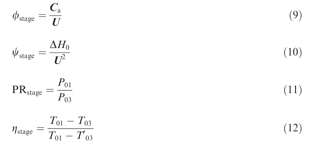
where subscript‘‘0”emphasizes that the property is associated with total condition (as opposed to static). The numerical numbers ‘‘1”, ‘‘2” and ‘‘3” indicates vane inlet, between vane and rotor,and rotor outlet respectively.ΔH0 is the total specific enthalpy extracted by the turbine stage. U is the meanline blade velocity.

As mentioned previously, meanline turbine aerodynamic modelling has been used for preliminary design of key turbine flow and geometric parameters, such as annuli geometry and blade angles. It is used during the aerodynamic conceptual design phase for its simplicity and reasonably accurate ondesign performance prediction, especially when analyzing designs of high hub-to-tip ratios.

Although the meanline turbomachinery modelling has previously been used for health monitoring purposes, such as the work of Ciccioti et al.,23to authors’ best knowledge, it has never been used for the assessment of fault severity, as in the case of this work, for the assessment of the blade surface roughness in an axial turbine.Instead of being used as a design tool,the objective of meanline modelling in the fault-assessing framework is twofold: (1) to analyze the performance of the components in an existing turbine design, and (2) to serve as a means to relate the observed performance deteriorations to the physical condition of the component. To achieve these two objectives, the following challenges and limitations must be addressed during the application of the meanline model:

(1) To represent an established turbine with 3D blade design,the meanline representation of the flow condition must be carefully calibrated and verified, such that the performance prediction by the meanline model adequately matches that of the actual 3D design.

(2) Since the meanline design method relies on empirical correlations for loss predictions,its efficiency estimation is only as accurate as the empirical models employed.The ‘‘experiential” factors of the empirical models for loss components may needs to be calibrated against performance data of similar blade design, in order to yield mode accurate prediction.A demonstration of this point is presented in Section 2.3.

(3) At off-design conditions, the flow properties, such as Mach number, blade-loading and incidence angle, vary significantly at different locations along the blade span.Despite the development of the off-design incidence loss prediction method, such as the empirical model by Moustapha et al.,24the dramatic variation of spanwise flow conditions may not be adequately represented by the 1D meanline model.

Despite these shortcomings,meanline modelling is versatile for implementing damage loss models, which are directly derived from the observations on damage effects through either empirical cascade testing or numerical simulation. The adaptability of damage models and the overall simplicity make meanline modelling an ideal tool for analyzing damage effects on a specific turbine under specific operating conditions.

The subsequent section presents the Jouini-Islam&Sjolander blade roughness loss correlation systems, one of the damage models developed for the AMDCKO loss system implemented for this work.

2.3. Roughness loss system for axial turbines

2.3.1. The original Jouini-Islam & Sjolander correlation

Various experimental measurements have been conducted in the past to understand the effect of roughness on blade-row performance. These works include Bammert and Sandstede,25Boyonton et al.26and Yun et al.,6which unanimously reported substantial efficiency deterioration with increased surface roughness. The surface roughness affects the flow over it in two ways: (a) it causes flow to transition form laminar to turbulent at a lower Reynolds number, and (b) it increases the turbine boundary layer skin friction coefficient.Due to the turbulent boundary layer and enlarged surface area, surface roughness also increases the local heat transfer coefficient.Using the low-speed experimental data by Kind et al.with reasonable extrapolations, Islam developed the loss correlation for roughened blades.11The surface roughness loss was attributed to an effect on the profile loss, and the following profile loss ratio was proposed:

where ΔYRthe incremental loss due to roughness and YPRthe profile loss including the roughness effect. KLcorrelated with the sand grain roughness-to-chord ratio (χ=ks/c).

Originally, Islam & Sjolander suggested applying KLdirectly to the profile loss corrected for compressibility and Mach number effects.Through CFD simulation using a single surface roughness configuration, Jouini et al. found that the incremental roughness loss, i.e., ΔYRfrom Eq. (13), decreases gradually as the Mach number increased, especially near the transonic region.12The compressibility effect had a different impact on the roughness incremental loss than on the profile loss. According to this observation, Jouini et al. proposed the following correction factor to account for compressibility effects on surface roughness loss:

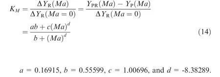
where ΔYR(Ma=0)is the incremental surface roughness loss calculated using Eq. (13), using the baseline profile loss without compressibility correction. ΔYR(Ma) is the incremental surface roughness loss at the outlet Mach number M.

2.3.2. Validation and modification of the Jouini-Islam &Sjolander roughness loss system

At the time Jouini et al. proposed the CFD-based compressibility correction factor for surface roughness loss, there was not yet any empirical data available for comparison and validation.Half a decade later,Yuan&Kind experimentally studied the effect of surface roughness on profile loss through transonic cascade testing,with a discharge Mach number from Mach 0.5 to 1.1.10Using the studies by Yuan&Kind,it is now possible to examine the effectiveness of the prediction method against the experimental outcomes. Since the Jouini-Islam &Sjolander roughness loss system is used in the proposed framework,it is also prudent to test it against the established experimental outcomes before incorporating them.

The measurement data by Yuan & Kind included profile loss and outlet flow angle at design incidence for both clean and roughened blades. The baseline turbine blade is the HS1C blade, which was designed by Corriveau & Sjolander based on the mid-span profile of an existing Pratt & Whitney Canada engine.27To simulate the roughness surface due to in-service damage, round natural silica sand grains with a nominal diameter of 90 μm, 165 μm , and 225 μm were used.The measurements for both smooth and roughened blades were made for discharge Mach numbers between 0.4 and 1.13. The corresponding Reynolds numbers were between 4×105and 1×106, which is the range where the profile loss becomes independent of Reynolds number.

The first part of the evaluation focuses on the roughness loss compressibility factor proposed by Jouini et al.KMvalues were determined for the measurements by Yuan&Kind for all the roughness cases, using the definition in Eq. (14). For each case, the incompressible roughness loss, i.e., ΔYR(Ma=0),was approximated using the measured YPand YPRvalues associated with the lowest Mach number, which was 0.5.ΔYRwas calculated by taking the direct difference between the measured YPR(Ma)and YP(Ma).Fig.1 compares the KMobtained from the experimental data with the CFD-based correlations.

The comparison shows that the CFD-based correlation trend agrees with the KMobtained from experimental data between Mach 0.5 and 1, confirming the decreasing trend of ΔYRwith Mach number, as observed by Jouini et al. Such a trend may be explained by the compressibility effects, which thin the boundary layer and suppress flow separation,causing a reduction in vicious losses.22Such a loss-reducing benefit certainly applies to the roughness loss effect.Despite trend agreement, the discrepancy in magnitude between the CFD-based predictions and empirical observations in this region was apparent. The CFD simulation underestimated the compressibility effects in the subsonic region, which was reflected by the higher KMvalues. The discrepancy between the measured and predicted results in this region of outlet Mach number was also reported by Yuan and Kind.10The shortcomings of the basic turbulence model in capturing the boundary layer phenomena contributed to the discrepancy, rather than the shortcomings of the surface roughness boundary-layer lawof-the-wall model employed.

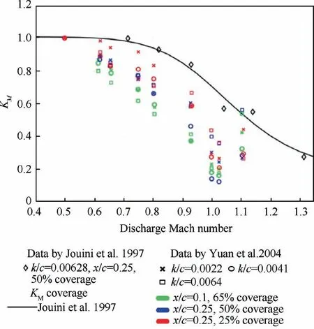
Fig. 1 Comparison of KM obtained using the experimental data of Yuan et al. with correlation by Jouini et al.

The KMtrend derived from the experimental data, as presented in Fig. 1, suggested a significant correlation with the chordwise roughness starting position (x/c) for an exit Mach number below unity.The low-speed experimental data showed that losses increased dramatically as the roughness strip was moved towards the leading edge; i.e., the lower the x/c value,the higher the ΔYRdue to a specific roughness height.11This may be caused by the extraction of a greater portion of momentum from the boundary layer by the roughness elements. The boundary layer was significantly thinner near the leading edge,as explained by Kind et al.9Yuan and Kind suggested that the earlier transition from laminar to turbulent flow induced by the roughness patch may also cause substantially greater overall loss production, as a greater portion of the blade surface becomes turbulent. Therefore, the trends of KMin Fig. 1 suggested that the loss-reducing benefit of the compressibility effect may be larger for blade surfaces with greater coverage of turbulent flow, caused by the earlier transition induced by the leading-edge roughness. Conversely, the KMtrends did not suggest a strong correlation between KMand roughness height, partially due to the high scatter, likely caused by experimental uncertainties.

The experimentally-derived KMtrends of different surface roughness configurations showed a rapid increase at Mach 1.1, and merged into the original KMtrend from the correlation by Jouini et al. Such rapid jumps are likely due to the dominance of the interactions between the shock and expansion waves developed near the trailing edge, as well as the boundary-layer affected by the surface roughness patches.The merging of the experimentally-derived KMbeyond an exit Mach number of 1.05 suggests that KMbecomes a weak function of x/c.

In light of the observation above,a modification was made to the KMcorrelation for an exit Mach number below 1.05,with the inclusion of the starting location of the surface roughness. Fig. 2 shows the KMtrend of the modified correlation,which is expressed in Eq.(15).

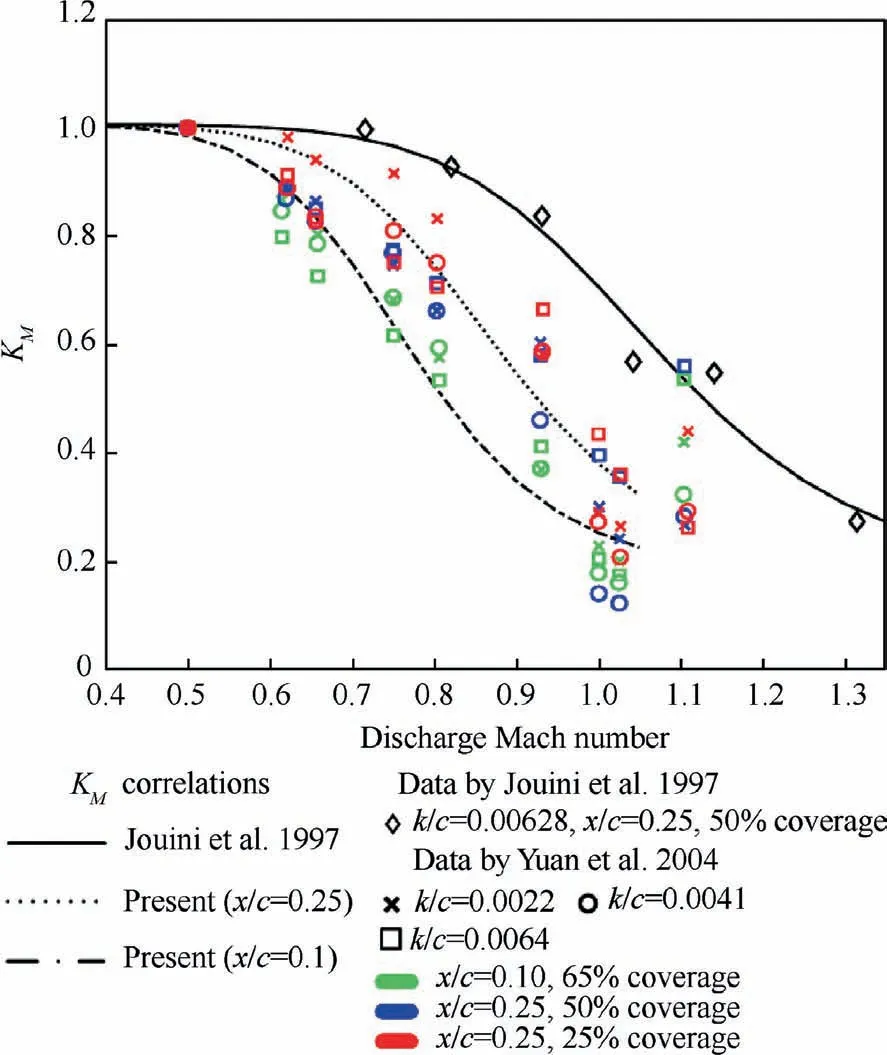
Fig. 2 Variation of KM with Mach number: comparison of empirical data with the modified correlations.

(for outlet Mach number between 0.5 and 1.05)

Following the validation and modification of the compressibility correction factor for roughness loss, the effectiveness of the roughness loss prediction system was examined. The baseline profile loss for the HS1C was predicted using the AMDCKO loss system for discharge Mach numbers from 0.5 to 1.2.The roughness loss for a selective amount of roughness configurations was then determined using both the original and the modified Jouini-Islam & Sjolander loss system.

Figs. 3 and 4 compare the roughness loss prediction with the measurement values by Yuan and Kind for the same roughness configurations.In general,the predicted incremental losses agreed with the experimental data, considering the experimental uncertainty margin. The predictions using the modified KMshowed superior agreement with the measurement data over the predictions using the original KM,and were well within the margins of experimental uncertainty for the medium rough band cases.For the narrow band cases,the predicted incremental losses using both the original and the modified KMshowed underestimation compared to the measurement values. This was especially significant for cases with smaller roughness heights, i.e., k/c=0.0022 and k/c=0.0041. Such discrepancies may be caused by the significantly large uncertainties associated with the measurement values,which were almost equivalent to the measured incremental losses in magnitude. The modelling errors associated with the Islam correlations may also have contributed to the underpredictions.Since the underpredictions took place at lower Mach numbers where the KMvalues are near unity,the underpredictions were unlikely due to the correlations for the compressibility factor. Despite the underpredictions, the predicted incremental losses using both the original and the modified KMwere still within the experimental error margins. The predictions using the modified KMstill showed closer agreements with the trend of the measured incremental losses.

For total pressure loss predictions, those using the original KMshowed better agreement with the measured values for an exit Mach number between 0.95 and 1.05, while the modified KMyielded underprediction. However, the comparison based on the total pressure loss coefficient can be deceptive, as the overprediction of the incremental loss by the original KM was compensated for by the underprediction of the baseline losses by the AMDCKO system for this Mach number range.

Based on the accumulated understanding of the meanline empirical-based roughness loss prediction, the following section presents the development of an online framework for surface roughness assessment of HP turbine blades on an inservice GTE.

2.4. The proposed online surface roughness assessment framework

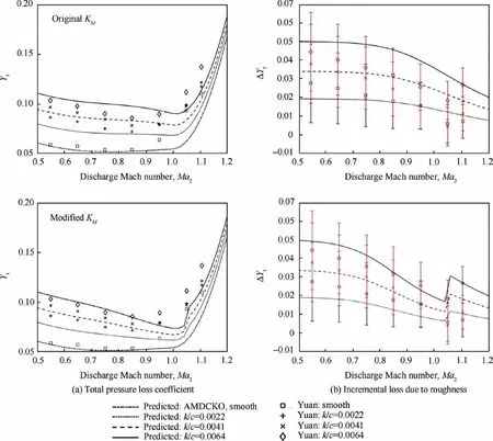
Fig. 3 Total pressure loss coefficient with medium roughness band (x/c=0.25, s/c=0.475).

As presented in the previous sections,GPA and meanline analysis were originally developed for GTE condition monitoring and turbomachinery preliminary design, respectively. Each has strengths and limitations when utilized for the new purpose of component-level fault assessment. The proposed online turbine surface roughness assessment framework aims to integrate these two methods in a way that can exploit the strengths while overcoming the limitations. To achieve this goal, the online assessment framework incorporated an interfacing process to alleviate measurement uncertainties and modelling shortcomings associated with GPA. A meaningful efficiency deviation trend corresponding to the growth of surface roughness could then be extracted and passed on to the meanline analysis. The meanline turbine model in the framework was established through a system identification approach, in order to best represent the flow conditions in the modelled turbine components.

The schematics diagram of the proposed framework is shown in Fig.5.The HP turbine surface roughness assessment routine starts with data acquisition using the instrumentation associated with the GTE’s control system, which typical acquires steady-state monitoring and operational data. The system-level GPA analysis will then be applied to the obtained data to identify the internal degradation state of the turbine subsystem, and the associated gas path parameters (GPP), as described in Section 2.1. Through the GPA-meanline interfacing process,elaborated on in Section 2.4.1,the efficiency deviation associated with the turbine surface roughness degradation will be extracted from the GPA results.The uncertainties with the steady-state GPA analysis will also be alleviated in this process. The extracted efficiency deviation will be passed on to the component-specific turbine meanline analysis,where the meanline aerodynamic model for the clean turbine is first identified and calibrated. The surface roughness fault severity is then determined using the received efficiency deviation.

2.4.1. GPA-meanline interfacing process

The proposed GPA-meanline interfacing process samples and transforms the GPA results,i.e.,GPP and η of the turbine subsystem, into a temporal trend of efficiency deviation tailored for the meanline roughness identification process.

The isentropic efficiency deviation caused by the surface roughness is determined by analysing the turbine performance characteristics’ transformation, i.e. efficiency and corrected mass flow curves, which deviate from the original baseline as the turbine deteriorates.As illustrated in Fig.6,different types of faults in the turbine components transform the performance curves distinctively,according to MacIsaac&Langton.28With the presence of a surface roughness fault, which is the main focus of the present framework, the efficiency curve shifts almost straight downward according to the observations.6,28,29The mass flow curve elevates marginally for a transonic turbine,due to the slight opening of the throat caused by erosion.

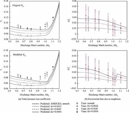
Fig. 4 Total pressure loss coefficient with narrow roughness band (x/c=0.25, s/c=0.25).

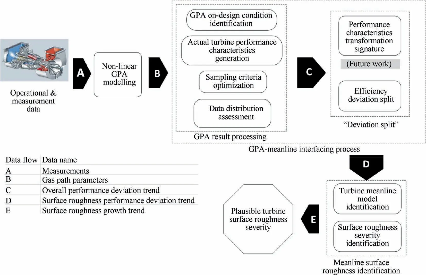
Fig. 5 Main components of online turbine surface roughness assessment framework.

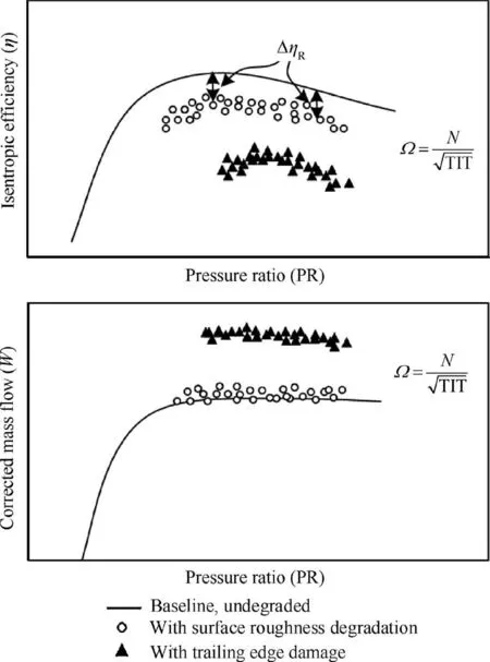
Fig. 6 Transformation of turbine performance characteristic curves associated with same Ω due to different faults, reproduced based on MacIsaac and Langton.28.

Accordingly, the isentropic efficiency deviation due to surface roughness (Δηt，R) can be approximated by the difference between the values from the baseline efficiency curve(ηt，baseline) and the efficiency curves established from the GPA results (ηt，GPA):

where Ω is the corrected rotor speed,which characterizes individual efficiency and mass flow curves in the turbine performance characteristics, and is defined with shaft speed (N)and turbine inlet temperature (TIT) as follows:

Therefore, the end goal of the GPA-meanline interfacing process is to determine the development of Δηt，Rover the operational history of the turbine for a particular Ω.To achieve this objective, the interfacing process samples relevant GPA result entries and reconstructs ηt，GPAthrough a series of steps. as shown in Fig. 7. This process can be divided into two parts:(1) the identification of the design TIT and N in the context of the GPA model,around which the GPA results will be sampled and(2)the strategic sampling process,which is optimized to address the uncertainties associated with the GPA while alleviating the fouling effect on the results.

To achieve both parts of the objective,the present interfacing process utilizes the outcomes of two GPA models, namely the ideal and the turbine-degrading models. An overview of the two models has been provided in Section 2.1, and a brief elaboration is provided here for the purpose of this discussion.The ideal model evaluates the expected power produced by the undegraded GTE by converging only on the recorded conditions at the boundary of the GTE,such as the compressor inlet temperature and pressure,and the EGT.It was originally used to calculate the power deficit, i.e. the difference between the expected power and the recorded value from the operating system, in order to capture the compressor fouling effect. The turbine-degrading model resolves turbine long-term degradation‘‘symptoms,”i.e.,deterioration of the isentropic efficiency and increase in mass flow, by scaling the turbine performance characteristics and matching the calculated power and EGT to the recorded values.Therefore,the efficiency and GPP analyzed using this model resemble the actual thermodynamic conditions in the GTE,due to the long-term degradation of turbine.Since the turbine-degrading model does not account for the compressor fouling effect, it should only be used within a limited time period after each compressor wash when compressor fouling effect is negligible.When analyzing the operating conditions affected by fouling,the model-assessed GPPs deviate from the actual conditions and should be considered physically invalid.The two models utilize the same set of thermodynamic equations for a GTE cycle and the same baseline component characteristic maps, only differing in algorithm. As seen in Fig.5,the interfacing process utilizes the results of both models according to the unique functionalities of both parts of the objective. For the convenience of discussion, the parameters associated with the ideal and the turbine-degrading model are denoted with single and double apostrophes,respectively.

The first part of the interfacing process aims to identify the design TIT,N,and ˙m in the context of the GPA model,which are used to establish the sampling criterion for collecting the GPA result entries corresponding to similar operating conditions.This is because the meanline method is the most reliable when analyzing the design condition.

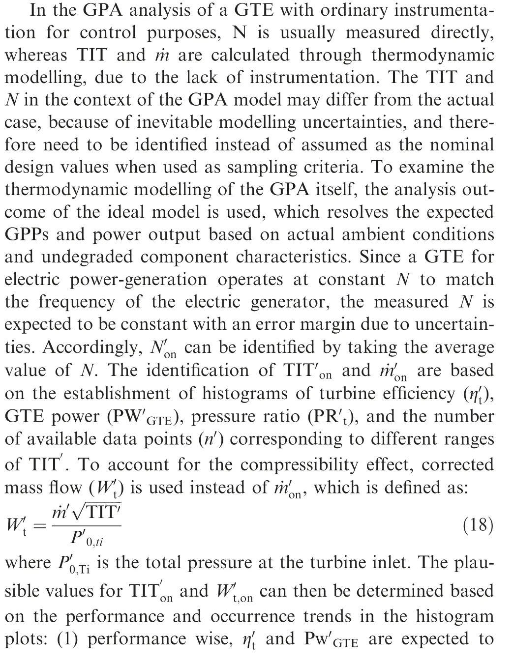
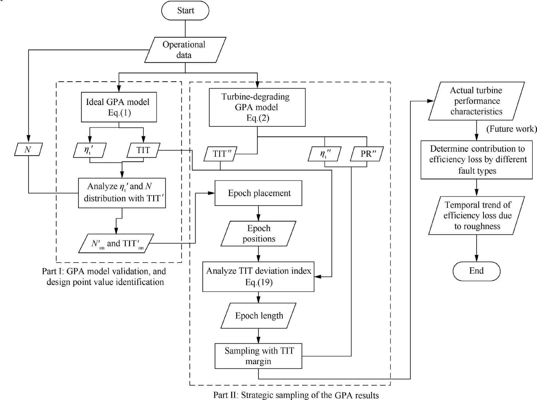
Fig. 7 Main steps of GPA-meanline interfacing process.

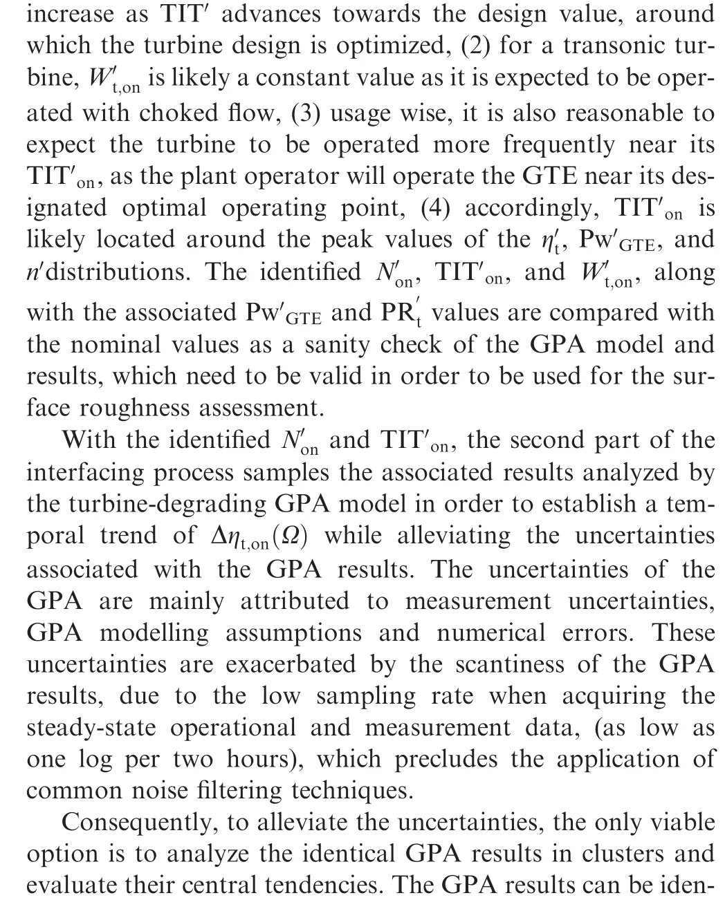
Epochs, i.e., sampling time windows, are placed at convenient times throughout the operational history of the GTE,such that the GPA results of the same period can be gathered and evaluated as a group. It is defined using two parameters:temporal position (εi) and epoch length (εT), which are the starting time and the time span of the epoch, respectively.The establishment of εiis dependent on the usage of the GTE. Due to the variations in ambient conditions, as well as power demands throughout a year, the operating range of an GTE may vary significantly between seasons, and as a result,the turbine may be running close tomore frequently for some periods during the year and rarely for others. Since the turbine-degrading GPA model is susceptible to compressor fouling when resolving the long-term turbine efficiency deterioration, the epochs are restricted to be placed immediately after the compressor wash,where the compressor is considered to be in mint condition. Based on the above, εiis in fact the compressor wash time after which the turbine has been running regularly near the TITon.

For each established εi, an appropriate εTis determined such that maximum entries of the GPA result can be sampled with minimal influence of compressor fouling. Physically, the fouling effect is not manifested as the compressor efficiency deviation for a short time period after the compressor wash,until reaching a ‘‘pivoting” point after which the efficiency deterioration becomes significant,as seen in a typical case presented in Fig.8(a).This observation indicates the existence of a time period after each compressor wash where the outcome of the turbine-degrading model is not yet affected by the fouling.Therefore, the optimal εTis established at the pivoting time after which the influence of fouling on the key parameters of the turbine-degrading GPA becomes significant.

To identify the pivoting time, the effect of fouling on the turbine-degrading GPA model by Hanachi et al.19is examined.The examination suggested the following plausible mechanism through which compressor fouling affects the model’s GPP estimation:

The turbine-degradation assessing algorithm attributes all the degradation effects to the turbine subsystem,and therefore does not account for the increased power consumption by the compressor with decreased efficiency due to fouling.Physically,as the compressor fouling effect becomes significant, the compressor consumes a higher portion of the power generated by the turbine, causing the recorded GTE power to deviate from the expected values.

The EGT, however, is not affected by fouling, since it is taken directly from the measurement and used as one of the convergence criteria, as seen in Eq. (2).

Consequently,while assuming undegraded compressor performance, the algorithm of the turbine-degrading GPA method matches the recorded EGT and GTE power by accounting for less turbine power extraction, which yields underestimated TIT and unrealistic ηtand Wt.

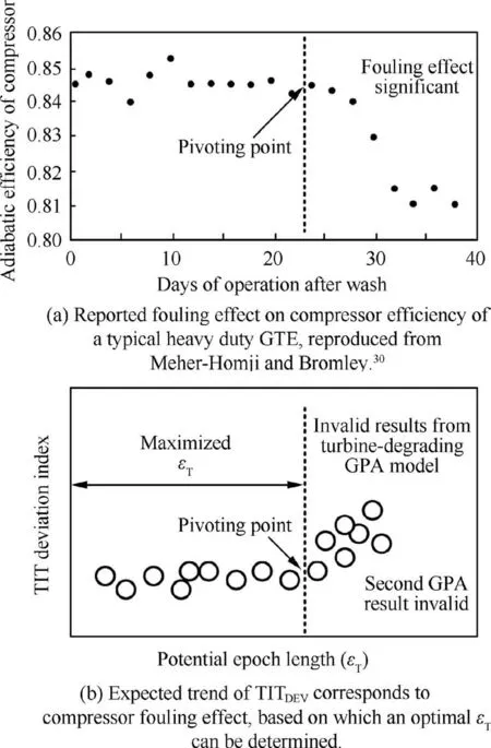
Fig. 8 Determination of optimal εT utilizing TITDEV index.

Therefore,for the GPA model as expressed in Eq.(2),TIT′′is the parameter directly affected by compressor fouling.According to this revelation, a ‘‘TIT deviation index”(TITDEV) is developed, in order to capture the pivoting point.The indicator is defined as the ratio of the TIT deviation to the expected TIT as follows:

where TITexpis the expected turbine inlet temperature of an undegraded GTE under the same operational condition.Fig.8(b)illustrates the expected trend of TITDEVcorresponding to the fouling effect and its intended functionality in determining the optimum εT. Since the ideal GPA algorithm evaluates the GPPs and the performance of the GTE in an undegraded condition,the TITexpin Eq.(19)is essentially the TIT′.

Once each epoch is established,the condition-oriented sampling criterion ‘‘TIT margin” (TITm) is established to gather GPA result entries associated with Ω′on.It is important to distinguish between operating conditions when relating degradation to efficiency deterioration, since the aerodynamic loss varies with flow conditions, such as Mach number and incidence angle.For example,Kind et al.9showed that the boundary layer was more susceptible to separation by surface roughness when the airfoil was operated at off-design incidences,consequently causing greater losses compared to those at the design incidence. The sensitivity of efficiency loss to the same surface roughness severity is also influenced by compressibility effects,as seen in Section 2.3.Therefore,operating conditions must be considered when attributing efficiency deviations to fault severities.

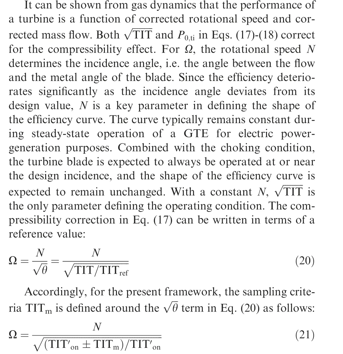
The selection of TITmis therefore dependent on its influence on the overall compressibility effect, which is determined by the magnitude of TITon. For example, for a high TITonof 1100 K at 16,500 RPM, a TITmof 10 K yields a 0.45% variation in the blade Mach number, which results in a negligible overall performance impact.

With the epochs intermittently placed throughout the operational history, results from the turbine-degrading model are sampled around the identified, through the sampling criterion TITm. The ηtand PRtof the sampled result entries for each period are then arranged into an efficiency curve, which is expected to deviate from the baseline in accordance with the degradation condition of the turbine for that period. Multiple efficiency curves corresponding tofrom different time periods can then be established, which in turn, reveal the temporal trajectory of the curve transformation from the baseline, as illustrated in Fig. 9. The temporal trend ofcan then be established using the approximation presented in Eq. (16).

It is important to note that, due to the lack of data in the open literature on the efficiency curve transformation trajectory in relation to fault types other than surface roughness,the Δηt，Rapproximation method in Eq. (16) could only be applied to GTEs. In these cases, surface roughness was the predominant cause of degradation,due to rugged blade design as well as less frequent and longer transient operations. Nevertheless, the transformational signature-based component-level fault feature extraction will be explored in the author’s future work,so as to extend the present framework’s ability to the assessment of multiple fault type severities. Examples include tip-clearance enlargement and trailing edge damage, which are more likely to occur in aeroengines and emergency power units.

2.4.2. Meanline surface roughness identification

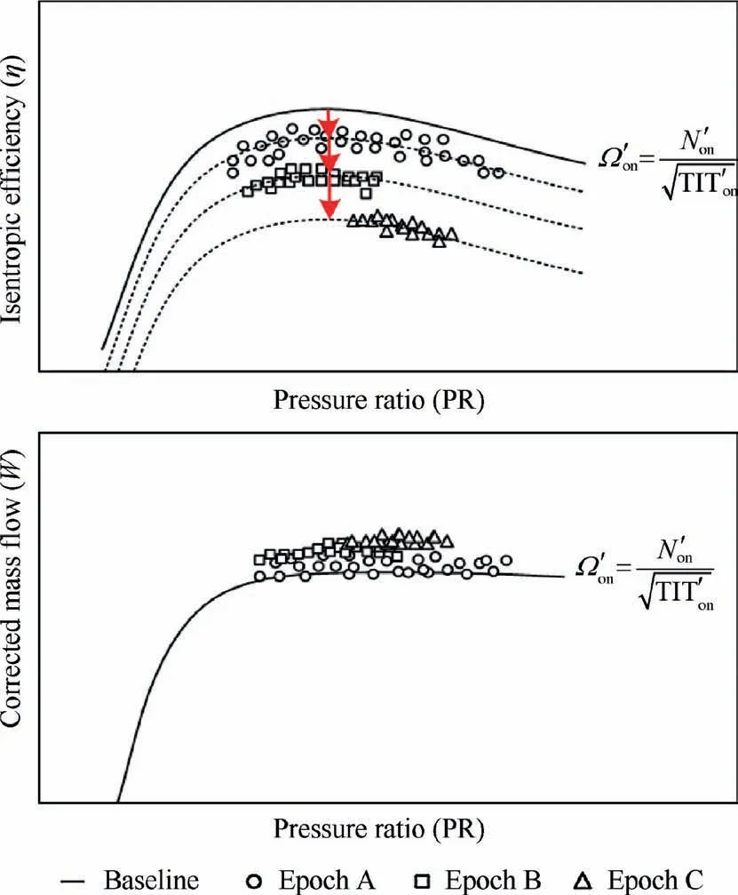
Fig. 9 Efficiency curves corresponding to same from different epochs reveal temporal trajectory of curve transformation due to blade roughening.

The meanline roughness identification process was developed to resolve the surface roughness severities from the extracted efficiency deviations.Different from the design-oriented meanline analysis procedure, the proposed identification process first established the mean-radii representations of the flow conditions across the span of the existing undegraded turbine. It utilized the nominal performance values and key design parameters,in order to assess the component losses associated with the original design. Based on the established meanline representative turbine model,the second part of the identification process matched the surface roughness severity to the Δηt，Robtained from the GPA-meanline interfacing process,which in turn, resolved the surface roughness growth trend.The details of the two-part identification process are shown in Fig. 10.

The first part of the identification process aims to establish the meanline representation of the flow conditions across the span of the HP turbine vanes and blades, such that the basic performance parameters of the model match the nominal values of the actual turbine.Although the availability of information on a particular turbine component varies, the minimum information required to establish the meanline model for an existing turbine design includes: (1) annuli gas path geometry,(2) basic blade geometry specifications, such as chord length,blade angles, stagger angle, solidity, and the maximum thickness-to-chord ratio, and (3) turbine inlet flow conditions,including flow angle, total pressure and temperature, in order to establish the velocity triangles, and consequently resolve the energy transfer by the turbine as well as the aerodynamic losses.To ensure that the meanline simplification model represents the actual turbine, key performance parameters, such as pressure ratio (PRstage), work coefficient (ψstage), flow coefficient (φstage), reaction (Λstage), and the isentropic total-tototal efficiency (ηstage) are also used as modelling constraints.The definitions of these parameters are presented in Section 2.2.

Since the surface roughness loss correlation model is a function of profile loss, as shown in Eq. (13), and the profile loss correlation of the AMDCKO system is correlated by relative flow angles,22the focus of the clean turbine meanline modelling should be on establishing accurate relative flow angles across the span. The profile loss assessment can also be improved by adjusting experience-based correction factors.

Depending on the complexity of the turbine design, as well as the availability of information on the design, iterative parameter adjustment varies for different cases and requires engineering judgement.

The second part of the identification process resolved the surface roughness severity by matching the damage correlation-incorporated meanline model to the efficiency deviations, i.e., Δηt，R（）obtained from the GPA-meanline interfacing process. The surface roughness loss prediction system presented in Section 2.3 was incorporated into the previously identified meanline model for the clean turbine. Since the surface roughness loss had a minimal effect on the outlet flow angles and provided that it did not result in substantial flow separation, according to the empirical observation of Kind et al.9and Yuan & Kind,10the velocity triangle deviation angles of the established meanline model were held constant.

Fig. 10 Proposed meanline surface roughness fault matching process for surface roughness severity associated with identified efficient deviation associated with an epoch.

As a proof-of-concept, with the objective low-fidelity assessment of surface roughness condition, a surfaceroughness-level index was created for the present work. The index was defined as the surface roughness height at 25%coverage starting at the 5%chord position from the leading edge.Since the surface roughness on the suction side of the airfoil has a significantly higher influence on the aerodynamic loss,according to the observation of Kind et al.,9the index was defined using the roughness level on the suction surface. The selection of 25%coverage was in accordance with the observations of the first stage HP turbine blades of two different aeroengines by Taylor,8which revealed the leading-edge area as the region with distinctively higher surface roughness severity compared to the rest of the suction surface. The index also assumed the same surface roughness height for vanes and blades. The identification process iteratively resolved the meanline surface roughness index by matching the efficiency drop predicted by the meanline model to the trend in Δηt，R（）, which was determined through the GPAmeanline interfacing process. For the convenience of discussion, this index is called ‘‘Quarter Surface Coverage Index”.In the subsequent section, the proposed online surface roughness assessment framework was applied to the threeyear operational data of an GTE in order to evaluate the feasibility of the framework.

3. Case study: SGT-100 HP turbine surface roughness assessment

The effectiveness of the proposed online turbine surface roughness assessment framework was examined through its application to the three-year operational data of a 4 MWe Siemens/Ruston SGT-100 ‘‘Typhoon” cogeneration GTE powerplant.This particular engine was selected as the subject of the study,due to the availability of a three-year operational log, as seen in Fig.11,as well as the extensive documentation of the engine and its turbine design in the open literature.The present study aims to assess the surface roughness level of the turbine blade through the developed framework using the logged measurement data from the operating system of the GTE.

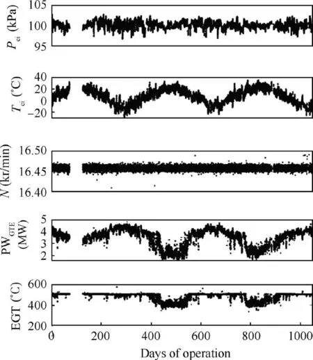
Fig.11 Variations of measured operating parameters over threeyear span of GTE’s operational history.

Due to a lack of observation data associated with this particular engine, the present validation was achieved using the available measurement values reported by Tarada,5which included the observation of several Ruston-manufactured HP turbine vanes and blades made of the IN939 alloy.

The nominal design values of the original introductory model of this engine are summarized in Table 1. The original turbine vanes and blades were manufactured with the IN939 alloy.31It should be noted that the Typhoon GTE series has been subjected to multiple design upgrades since its introduction. For example, the turbine inlet temperature has been reportedly raised to 1100°C, which consequently increased power output,mass flow rate,pressure ratio,exhaust gas temperature, and thermal efficiency.32

The geometry and performance of the HP turbine were obtained from Hannis et al.33The meanline modelling used the annuli geometry as well as the measured performance of the turbine stage, which are presented in Fig. 12 and Table 2,respectively.

3.1. Source of data and GPA results

The measurement and operational data provided by the plant operator includes date and time (t), Tci, Pci, EGT, N, PWGTE,fuel pressure and fuel valve angle.A selection of them are plotted in Fig. 11. The data were logged every two hours between 2008 and 2011,except for the period between June and August of 2008, when the GTE was shut down according to the plant operator. The EGT, Tciwere acquired from a total of 44 sensors for each log entry,and the average value of the redundant measurements were used for analysis.

The operational data were processed by both the ideal and the turbine-degrading GPA model developed by Hanachi et al.18,19,34For both GPA analyses, 37 parameters areresolved for each entry of operating history. These include GPPs of the main GTE subsystems, i.e. compressor, combustor and turbine, as well as the overall performance of the GTE. Among these parameters, the surface roughness assessment framework uses PWGTEand N of the GTE, as well as the thermodynamic conditions associated with the turbine subsystem. These conditions include TIT, PRt, ˙mtand ηt. Fig. 13 shows the variation of these parameters over the three years of the GTE operation for analysis using both GPA models.Based on these data,the subsequent section demonstrates the process of forming a condition-specific efficiency deviation trend for meanline surface roughness identification.

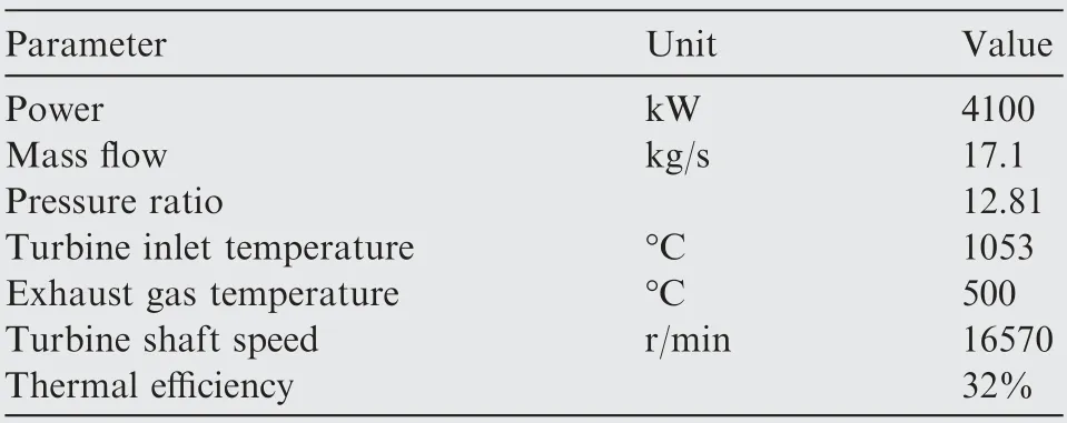
Table 1 Basic performance of original Ruston Typhoon GTE.31

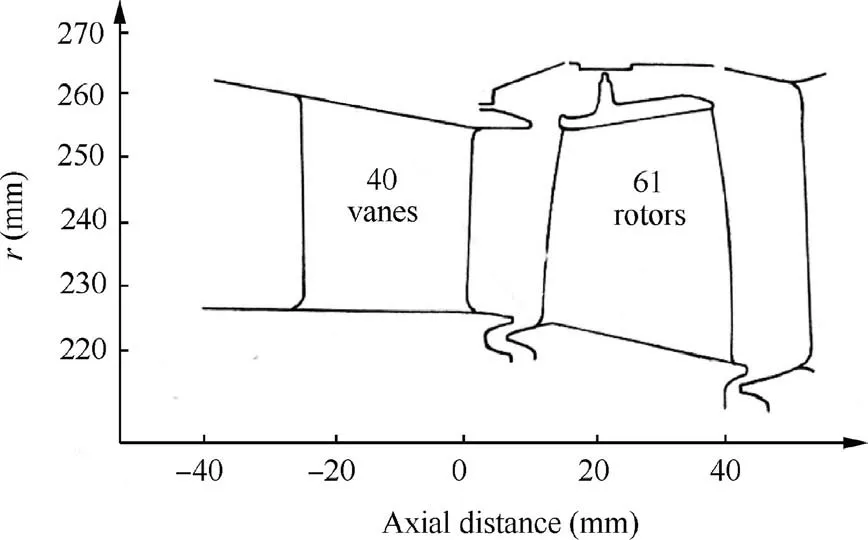
Fig. 12 Flow path geometry of the HP turbine stage, adapted from Hannis et al.33.

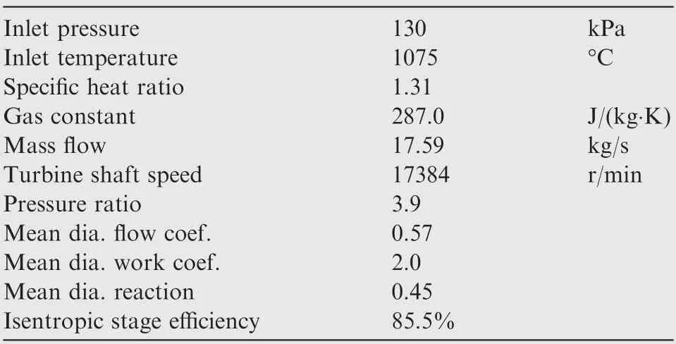
Table 2 Nominal performance for HP turbine of Typhoon GTE.33

3.2. GPA-meanline interfacing process

As a co-generation GTE, the value of N throughout its operational history was relatively constant,as seen in Fig.11.Closer examination of this vector shows that the value of N ranged from 16,411 to 16,519 RPM, with a mean and median of 16,458 RPM. Based on this observation, the on-design N′was considered to be constant at 16,458 RPM,and as a result,the variation of TIT′predominantly effected the value of Ω.Therefore,the performance curves of the turbine in the present GTE were characterized by the variation in the compressibility effect.

Fig. 14 shows the temporal variations of various performance parameters and occurrences with TIT′, i.e., the ideal GPA value. Based on this observation, two candidate values for TIT′onwere identified based on the ‘‘peak efficiency” and the ‘‘maximum occurrence” criteria specified in Section 2.4,which were 1090°C and 1095°C, respectively. Due to a lack of information on the ‘‘Typhoon” variant studied, there were no specific comparable nominal values apart from those in the literature. Nevertheless, Fig. 14 shows that the identified values were within reasonable range of the reported TITonof the improved model, i.e., 1100°C, and the associated performance parameters were sufficiently close to the nominal values summarized in Table 1. This demonstrates the validity of the thermodynamic model used in the GPA. The corrected mass flow, W′t, was a constant line, indicating the choking of the turbine for all ranges of TIT′. Since both N′and W′twere relatively constant,the incidence angle of the rotor,which significantly affects the losses,was also considered constant.Around the baseline TIT′onvalue of 1090°C, a TITmof 10°C was selected, which led to a TIT′sampling range between 1080°C and 1100°C, corresponding to ±0.37% variation of the compressibility correction term

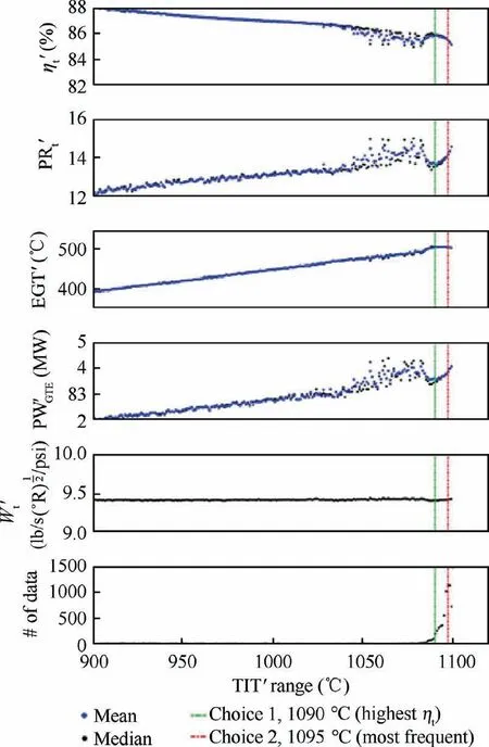
Fig. 14 Identification of TIT′on based on results of Ideal GPA Model.

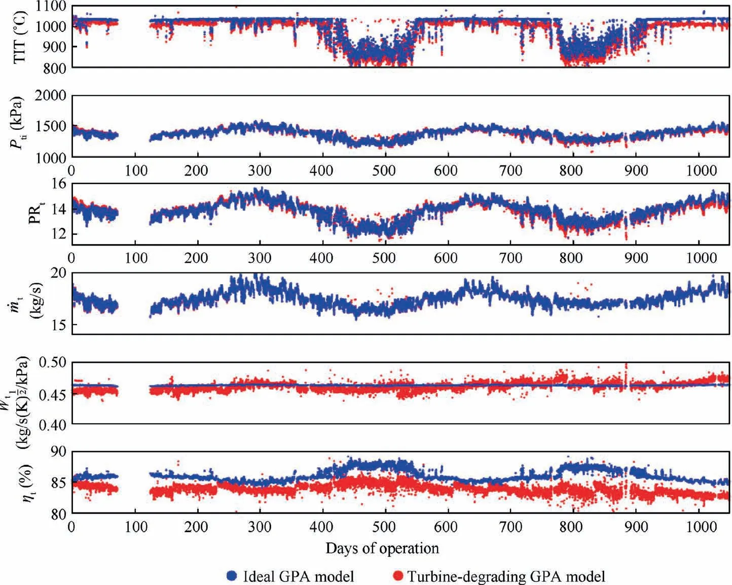
Fig. 13 Gas path parameters estimated by both ideal and turbine-degrading model.

Fig. 15 shows the epoch placement throughout the operational history. The establishment of εiwas based on the available data corresponding to the defined TIT′range near each wash, which can be clearly visualized in Fig. 15(b). Table 3 summarizes the detailed εiestablishment for each epoch. The GTE rarely operated near the identified TITonin the summer season,due to the lack of demand for electric power and heat.

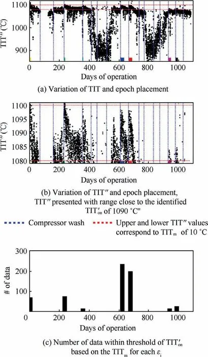
Fig.15 Epoch placement based on TIT′on=1090°C with TITm of 10°C for results of Turbine-degrading GPA Model.

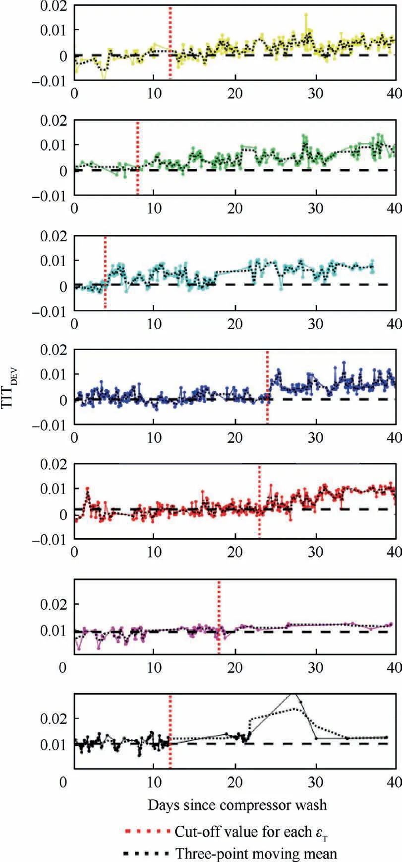
Fig. 16 TITDEV variation indicated effects on TIT′′ due to both short-term fouling, and long-term turbine degradation.

Table 3 Epoch placement and corresponding time in operational history.

The epoch length, i.e., εT, was determined through examination of the TITDEVindicator corresponding to each epoch.As seen in Fig. 16, the TITDEVvariations of epoch ε1to ε5clearly indicated the fouling effect on the TIT′′evaluated by the turbine-degrading GPA model. The time right before the deviation in TITDEVwas used as the value of εT. The starting baseline value of TITDEVfor ε6and ε7were both 0.01 instead of zero,indicating the effect of the long-term turbine degradation on the TIT′′.Physically,a GTE with a degraded turbine is expected to be operating at a lower TIT,due to the EGT limit imposed by the control system, as the turbine can no longer extract the same amount of energy for a given pressure ratio.Therefore, the lower TIT′′evaluated by the turbinedegrading GPA algorithm was valid and reflects the actual TIT.Since the TIT′′of ε6and ε7were close to the lower bound of the sampling criteria, the entries with deviated TIT′′due to fouling effects were excluded from the sample.Contrary to the linearized fouling model proposed by Hanachi et al.20, the observation of TITDEVsuggested a nonlinear fouling behaviour,which included a limited period where the fouling effect was not yet manifested as performance deterioration symptoms. This, however, is in accordance with the observations reported by Meher-Homji and Bromley.30

After establishing the epochs, the results from the turbinedegrading GPA were sampled and reconstructed into turbine performance characteristics, which are shown in Fig. 17. The overall near-level slope of the constructed efficiency curves indicated that the sampled result entries were around the peak efficiency region of the curve. The colour-coded curves of different epochs revealed the gradual downward translation of the efficiency curve,as well as the modest elevation of the corrected mass flow over the operating history. The turbine performance curve transformation was consistent with the transformational signature of a turbine with a surface roughness fault, as suggested in Section 2.4.1. This revelation was backed by the early testing results of the Typhoon prototype,after which the examination of the turbine seal strips confirmed the absence of blade rubbing during GTE operation.35Combining the observations above, it was reasonable to exclude the tip-clearance enlargement from being a potential degradational fault and instead the turbine blade surface roughening was considered the predominant cause of the efficiency deviation.

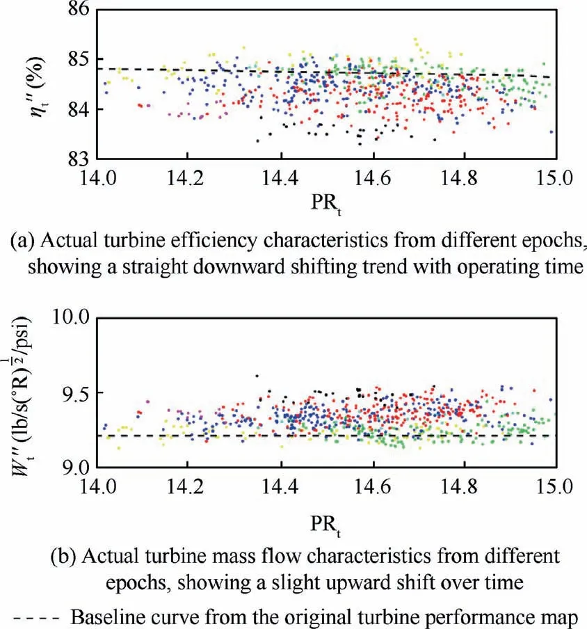
Fig. 17 Constructed turbine performance characteristics utilizing sampled results of different epochs from Turbine-degrading GPA Model.

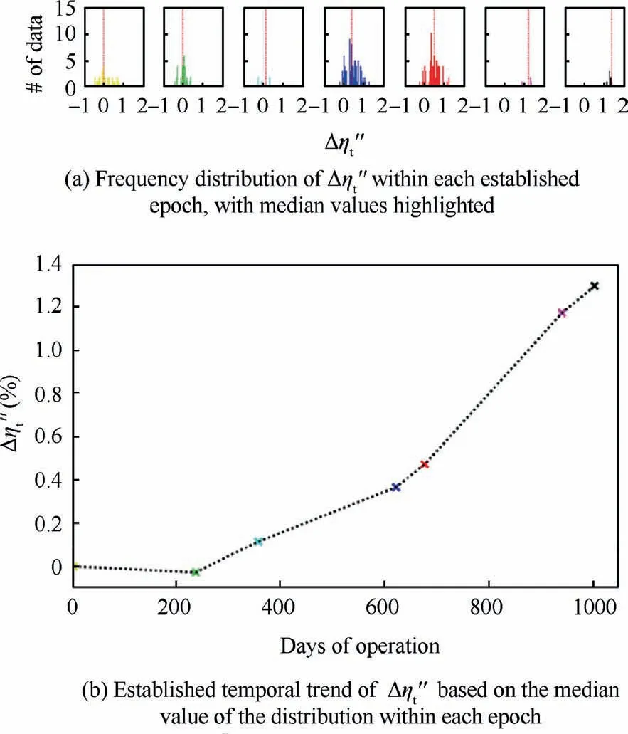
Fig. 18 Formulation of temporal trend of Δη′′t utilizing median value of its distribution within each epoch.

The turbine efficiency deviation, Δηt, was calculated for every sample using the approximation outlined in Eq.(16).Fig. 18(a) shows the frequency distribution of Δηt. For all epochs other than, the distribution of Δηtappeared binomial,for which the median was considered representative. Due to small εT,the distribution of ε3was unclear and the mean value was taken as representative.Fig.18(b)presents the established Δηttrend with the time of operation. From previous discussions on the transformation of turbine characteristics, as well as the reported observations during prototype testing, the Δηtgrowth trend was fully attributed to the surface roughness degradation of the present analysis.It was passed on to meanline severity identification without further processing.

Fig. 19 compares the efficiency loss ‘‘symptom,” ζη,obtained by the present epoch-based sampling method to the original result by Hanachi et al.,34which was obtained using a fixed five-day sampling period after each wash without distinguishing between operating conditions. ζηwas defined as the ratio of efficiency deviation to the actual efficiency. With an extended sample size and condition-based sampling criteria,ζηassessed by the present interfacing process showed a relatively modest and gradual growth trend compared to that by Hanachi et al. The difference was likely due to the following two reasons: (1) compared to sampling periods greater than 10 days, a five-day sampling period was still insufficient at gathering enough data to form a clear distribution of ζηand(2) without distinguishing between operating conditions, i.e.,TIT, the distribution of ζηwill be influenced by the result entries associated with a TIT significantly lower than TITon,resulting in differences in corrected rotor speed and loss-toroughness sensitivity.

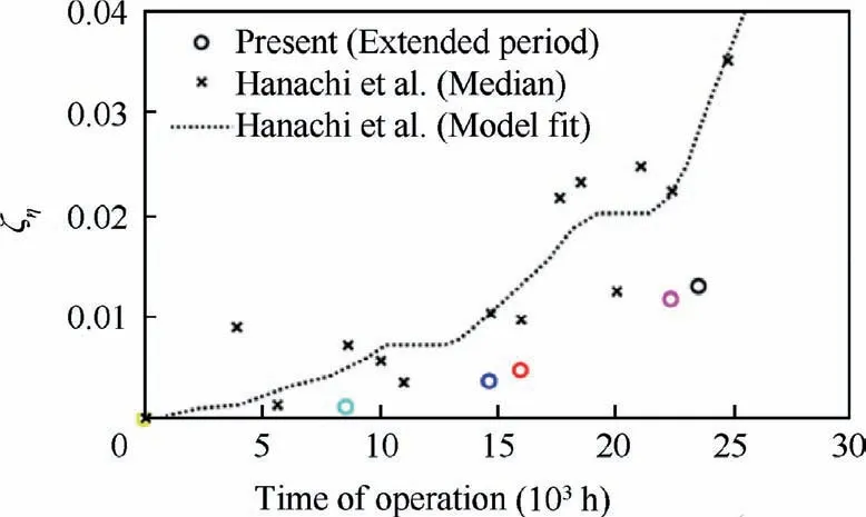
Fig. 19 Comparison of the ζη trend obtained by present interfacing process with previous results by Hanachi et al.34.

3.3. Meanline roughness identification for the HP turbine

Using the design choices and rig-test performance outcomes summarized in Section 3.1, a meanline aerodynamic model was established for the HP turbine of the Typhoon GTE.Using the methodology presented in Section 2.4, the meanline representative velocity triangles were adjusted based on the streamline curvature throughflow analysis outcomes,such that the calculated performance characteristics matched the reported values in Table 2.Fig.20 shows the final velocity triangles for both the established meanline model and the original streamline curvature outcomes presented in Hannis et al.33The assumptions used to establish the meanline velocity triangles are also presented.Table 4 summarizes the total pressure loss coefficients for various component losses associated with the AMDCKO loss system. As seen in Table 4, apart from the flow coefficient, the calculated values were within 1% agreement of the reported design and test rig values.

Fig. 21 shows the isentropic efficiency loss trend with the‘‘Quarter Surface Coverage Index” defined in Section 2.4.2 in terms of Ra for the HP turbine. At first glance, the efficiency drop may appear too optimistic compared to the efficiency drop reported in the literature, such as the 7% drop for ks/c of 0.01 by Bammert & Sandstede,25and the 19% drop for ks/c of 0.0067 by Yun et al.6However, the Mach number ranges corresponding to these two reported cases were extremely low, with nearly no compressibility effects, which have a large impact on the roughness incremental loss,as previously shown in Fig. 1.

Finally, the growth trend of the surface roughness in terms of the ‘‘Quarter Surface Coverage Index” is presented in Fig. 22. Blade samples were unavailable from the operator,so the assessed trend and magnitude of the index were compared with the measurements by Tarada,5which included the operating history associated with each blade sample. Among the measured data,there are a handful of IN939 blade samples from the HP turbine stages of the engines by Ruston,the original designer and manufacturer of the Typhoon GTE. Thus,the data associated with Ruston blade samples are highlighted.

To make the present results comparable with other IN939 measurements, an initial centre-line average surface roughness of 40 microns was assumed. Fig. 22(a) shows the surface roughness index,in both trend and magnitude agreement with the measured values from the Ruston IN939 samples. Fig. 22(b) compares the assessed surface roughness index with all available measurements by Tarada. The comparison shows that the surface roughness index of the monitored turbine reached the peak magnitude level shown in the measured data as the operating time of the GTE approached the recorded engine-core overhaul.

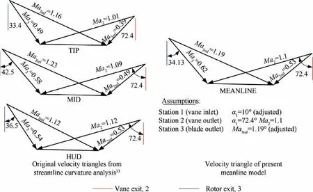
Fig. 20 Established meanline velocity triangles compared with the streamline curvature velocity triangles presented in Hannis et al.33.

Table 4 Assessed total pressure loss coefficients for various loss components.

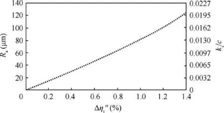
Fig.21 Variation of the‘‘Quarter Surface Coverage Index”with isentropic efficiency deficit.

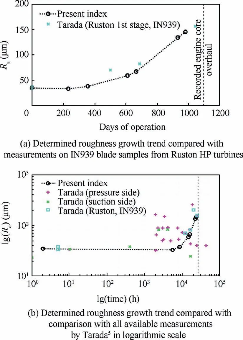
Fig.22 Growth trend of surface roughness in terms of‘‘Quarter Surface Roughness Index”, compared with available measurements by Tarada5.

4. Future potential improvements

The present surface-roughness indicator only serves as a lowfidelity, proof-of-concept assessment, as it was developed based on the exhaustive utilization of both logged operational data and literature. The indicator attributes all roughness damage loss to 25% of the surface area on the suction side near the leading edge. While such an indicator definition can provide some physical insight on the roughness condition of the turbine blade,it does not reflect the variation of roughness severity on the blade surface, especially for the pressure side where the in-service roughness damage is reportedly more severe.8A more advanced definition of an indicator is required to further quantify the surface roughness level at various locations on the airfoil, especially for associating the surface roughness indication with component failure.

The meanline modelling approach may be replaced by the 2D throughflow analysis. In general, 2D throughflow analysis is a better reverse-engineering tool compared to meanline modelling by accounting the radial pressure gradients and the spanwise variation of flow conditions. From the perspective of damage modelling, the 2D analysis also allows damage effects to be concentrated at a specific span location, as opposed to the present approach where the damage effects are averaged across the span. Such a 2D-based ‘‘concentrated” damage modelling approach has been successfully demonstrated by Klein in simulating the tip-clearance damage effects, which resulted in more realistic predictions of the spanwise temperature distributions and the overall efficiency penalties caused by the damage.36Klein’s work shows promise in incorporating such an approach of damage effects predictions into the framework.

In the discussion on the GPA-meanline interfacing process,a fault feature extraction concept based on the turbine performance characteristic transformation was briefly mentioned.Although realization of the performance characteristic transformation by different fault types was made almost three decades ago by Isaacs,37no specific publications exist in the public domain to establish such a link. A future investigation might focus on developing such a correlation, which allows for the expansion of the framework to the assessment of other fault types, including trailing edge damage and tip-clearance enlargement.

5. Conclusion

In this work, a physics-based online assessment framework was developed to assess the surface roughness level of the HP turbine in a GTE. It integrated the advantages of both GPA and meanline turbine modelling.

Since the meanline modelling component of the framework utilized the Islam & Sjolander empirical roughness loss correlations11as well as the compressibility correction factor for roughness loss proposed by Jouini et al.,12the validity of the correlations was first evaluated. The validation was based on the recent transonic roughness loss measurements by Yuan&Kind10using the HS1C transonic cascade.Yuan’s data confirmed the CFD-based observations by Jouini et al.,that is,the incremental loss due to roughness diminishes as the Mach number is increased. A modification was made to the compressibility correction factor based on Yuan’s data, which resulted in improved roughness loss prediction. Despite the deficiencies in the prediction of the baseline profile losses by the AMDCKO loss system,the predicted roughness incremental losses showed acceptable agreement with the measured results.

The components of the proposed online framework were then presented. In the GPA-meanline interfacing process, an epoch-based sampling method,as well as the turbine inlet temperature deviation indicator, i.e., TITDEV, were proposed to alleviate the uncertainties associated with the GPA outcomes,based on basic GTE instrumentation.A process was proposed for the development of the meanline-based surface roughness index for a specific turbine design.

The effectiveness of the proposed online-assessment framework was demonstrated by an application to GTE operational data over a three-year period between two major overhauls.The proposed TITDEVindicator clearly revealed the nonlinear behaviour of the fouling influence on the GPA results and was effectively used to maximize the acquirable sample size for each established epoch. With increased sample size and condition-specific sampling criteria, the interfacing process was able to alleviate the uncertainties associated with scantiness of data and different operating conditions. This, in turn,yielded a different observation on the performance deterioration symptom compared to the value reported by Hanachi et al.34on the same set of data. Finally, the growth trend of the proof-of-concept ‘‘Quarter Surface Coverage Index” was determined for the entire three-year operating period. The index showed both trend and magnitude agreement with the available measurement values of comparable blade samples reported by Tarada,5demonstrating the validity of the proposed surface roughness assessment approach as well as its potential as an effective online monitoring tool.

Declaration of Competing Interest

The authors declare that they have no known competing financial interests or personal relationships that could have appeared to influence the work reported in this paper.

Acknowledgements

The authors would gratefully acknowledge Dr. Steen A.Sjolander from Carleton University for his contribution over the course of this work.This project was supported by the Life Prediction Technologies Inc.(LPTi)and Natural Sciences and Engineering Research Council of Canada.