Transition prediction and sensitivity analysis for a natural laminar flow wing glove flight experiment

Tiho YANG, Hi ZHONG, Yifu CHEN, Yyun SHI, Junqing BAI,*,Feifei QIN

a Northwestern Polytechnical University, Xi’an 710072, China

b Chinese Flight Test Establishment, Xi’an 710089, China

c Xi’an Jiaotong University, Xi’an 710049, China

d ETH Zu¨rich (Swiss Federal Institute of Technology in Zu¨rich), Zu¨rich 8093, Switzerland

KEYWORDS eN method;Flight experiment;Natural laminar flow;Sensitivity analysis;Transition prediction

Abstract Natural laminar flow technology can significantly reduce aircraft aerodynamic drag and has excellent technical appeal for transport aircraft development with high aerodynamic efficiency.Accurately and efficiently predicting the laminar-to-turbulent transition and revealing the maintenance mechanism of laminar flow in a transport aircraft’s flight environment are significant for developing natural laminar flow wings. In this research, we carry out natural laminar flow flight experiments with different Reynolds numbers and angles of attack. The critical N-factor is calibrated as 9.0 using flight experimental data and linear stability theory from a statistical perspective,which makes sure that the relative error of transition location is within 5%. We then implement a simplified eN transition prediction method with a similar accuracy compared with linear stability theory. We compute the sensitivity information for the simplified eN method with an adjointbased method, using the automatic differentiation technique (ADjoint). The impact of Reynolds numbers and pressure distributions on TS waves is analyzed using the sensitivity information.Through the sensitivity analysis, we find that: favorable pressure gradients not only suppress the development of TS waves but also decrease their sensitivity to Reynolds numbers; there exist three special regions which are very sensitive to the pressure distribution,and the sensitivity decreases as the local favorable pressure gradient increases. The proposed sensitivity analysis method enables robust natural laminar flow wings design.

1. Introduction

To improve the fuel economy and to reduce environmental impact, novel technologies, such as composite material structures,1laminar flow wings,2active aeroelastic wings,3and adaptive structures,4have been proposed. Since the friction drag can be up to 50%of the total drag for a typical transport aircraft and the friction drag in a laminar boundary layer is much smaller than that of a turbulent boundary layer,laminar flow wing is one of the most promising technologies in future drag reduction. Research has shown that if 50% laminar flow is achieved on the wing upper surface, the drag could be reduced by 4.5%.5

Laminar-to-turbulent transition has complex physics.Nowadays, the Computational Fluid Dynamics (CFD), wind tunnel test, and flight test are used to reveal the transition mechanisms and design laminar flow wings.6–8.Both wind tunnel tests and flight tests can verify the reliability of the CFD method, and provide valuable data for improving the CFD method. The developed CFD method is then applied to aerodynamic shape design,which can save a lot of time and costs.9

Understanding the influence of base-flow distortions on stability is essential for robust reliable design. For instance, Reynolds number, turbulent intensity, and pressure coefficient all affect the flow within the boundary layer, and as a result they affect the associated instability growth rate10as well. Thus, it motivates an investigation of the sensitivity of instability waves with respect to base flow distortions. The research requires a reliable numerical transition prediction method which shall be verified by experimental data. In addition, an efficient sensitivity analysis approach is required to address large number of design variables.

Nowadays, various CFD based transition prediction approaches have been established, which can be categorized broadly into four types: (A) Direct Numerical Simulation(DNS),11(B) Large Eddy Simulation (LES)12based transition simulation approach,(C)statistical modeling approach,13,and(D) stability theory approach.7,14,15The last two approaches are based on Reynolds-Averaged Navier-Stokes (RANS) solver. Among all CFD based methods, the last two approaches are widely used because they have a good compromise between accuracy and computation cost.

Compared with the modeling method,the eNmethod based on stability analysis is more widely used in industrial applications.That is because the modeling method is not able to capture all the relevant physics.For example,for Langtry-Menter methods,14the physically-relevant upstream flow history is not taken into account; for Amplification Factor Transport(AFT)15method,there is a lack of cross-flow instability prediction. On the contrary, the eNmethod takes the upstream flow history into consideration,and it is also able to predict CF vortices.The eNmethod is based on the stability theory which captures the amplification stage of small disturbances along the streamwise direction in the laminar boundary layer from a physical point of view.8The eN-based methods can capture the evolution of relevant physical parameters in the flow field upstream of the transition point,which can reveal the physical mechanism of transition to some extent. Also, eN-based methods can predict both TS waves and CF vortices. So far, many theoretical and experimental researches have proven that eNis one of the most suitable techniques for engineering application research.

The Linear Stability Theory (LST), which is derived from linearized unsteady Navier-Stokes equations and neglects non-local and non-parallel effects, is usually used for eNmethod.6,16–20The LST approach is time-consuming and requires specific knowledge,as well as user intervention.Motivated by the need for a simple, accurate, and fast prediction tool, database methods based on LST, such as simplified eNmethod, are developed and applied.21–23

eN-based methods are widely implemented in different solution framework,such as the unstructured CFD solver,16,17FUN3d solver,24and the structured open-source ADflow solver.Seitz et al.25applied eN-based methods in a Natural Laminar Flow (NLF) forward-swept wing design for short- and medium-range transport applications where the Reynolds number is around 25 million. Based on eNmethod, Campbell and Lynde26designed a transonic NLF wing for a wind tunnel model at high Reynolds number. Cella et al.27successfully designed the UW-5006 transonic NLF wing by using the eN-based tool and validated the design results by wind tunnel test.The French Aerospace Lab carried out a wind tunnel experiment and performed CFD investigations with eNmethod focused on transition and performance predictions of a laminar wing28.Shi et al.18,19built an effective transition prediction tool based on linear stability theory with the RANS solver for three-dimensional configurations. The transition prediction results match the wind tunnel experimental data very well.

Combining numerical methods and wind tunnel tests is a widely used research approach for NLF wing design.However,limited by the size of the wind tunnel test section,the test Reynolds number is usually below 10 million,which is much lower than the typical Reynolds number of the transport aircraft.Although utilizing pressurization and hypothermia technologies can increase the wind tunnel Reynolds number to about 20 million, the turbulence level also becomes higher than that in a regular flight environment. For instance, NASA designed a supercritical NLF wing based on the Common Research Model(CRM)and tested it in the National Transonic Facility(NTF) with Reynolds number around 20 million.29,30However, because of a relatively high turbulence level, the critical N-factor of TS waves is around 6, which is much smaller than N-factor used for regular flight conditions. Thus, those data are not directly useful to verify CFD results for laminar flow wing design with high Reynolds numbers.

The above discussion motivates conducting flight test for verification and improvement of the CFD tool. The previous flight test does not cover all flight scenarios. Actually, most previous flight tests for the natural laminar flow control were conducted near cruise conditions, which cannot fully reflect the transition phenomenon of natural laminar flow control under flight conditions. Therefore, a flight test with high Reynolds number and different angles of attack is required.

With a reliable transition prediction tool validated by the flight test, we can design the NLF wings and develop sensitivity analysis approaches to understand key insights of laminar flow control. For instance, the TS waves are generated inside the boundary layer by freestream turbulence and are sensitive to the Reynolds number and pressure coefficient gradient. An understanding of how Reynolds number and pressure coefficient gradient affect transition is essential for NLF wings design.

Adjoint-based techniques can be used for sensitivity analysis of laminar-to-turbulent transition.They have been adopted for a wide range of computational studies in flow control31,32and shape optimization.33–35In recent work,we use Automatic Differentiation(AD)method36for the sensitivity of amplification factor(N-factor)to modification in the base flow,such as Reynolds number and pressure coefficient. Similar work has been performed for numerical research at low Reynolds number only. For example, Park and Zaki10researched the sensitivity of modal growth rates and N-factor to base-flow distortions in high-speed boundary layers with low Reynolds number below 10000. Pralits et al.37examined the flow response to surface disturbance and momentum sources by parametric analysis method.Similar studies have not been conducted at high Reynolds number.Besides,these researches did not carry out sensitivity analysis of NLF wings from a robust design view.

In the present work, we conduct a wing glove flight experiment at high Reynolds number and apply ADjoint-based sensitivity analysis to research the robustness of a natural laminar flow control wing.The flight tests are performed under a range of flight conditions in a flight envelope relevant to transport aircraft.The transition prediction method based on eNmethod is verified by a common research model and the flight tests and used to reveal the development of TS waves.The present work uses automatic differentiation for sensitivity information computation. The differentiated eNmethod, including a laminar boundary-layer code and stability analysis, is used to analyze the sensitivity of N-factor with respect to the pressure coefficient and the Reynolds number.

The paper is organized as follows:We start by a description of the flight experiment in Section 2. We then introduce the transition prediction method based on eNmethod and the derivative computation in Section 3. In Section 4, the critical N-factor is calibrated, and the transition prediction results are discussed. Sensitivity analysis under different flight conditions are shown in Section 5 and summarized in Section 6.

2. Description of flight test

2.1. Flight test platform and test matrix

The flight test is designed to advance the natural laminar flow control wing concept under operational conditions for typical transport aircraft and provide high-quality data for evaluating the physical processes associated with the TS waves to validate computational transition models.A business jet aircraft with a wing glove tested construct is chosen to carry out the flight experiment, as shown in Fig. 1. The sweep angle of leading edge is 5◦. Since TS instabilities dominate the transition on low sweep wings, we mainly research TS waves for this test.

The wing glove consists of a test section and two fairings.The purpose of fairings is to achieve a smooth connection in geometry between the test section and the main wing,ensuring acceptable stall characteristics at low speed.As the key part of the wing glove, the test section is formed by one single designed NLF airfoil, as shown in Fig. 2. The chord at the mid-span of the test section is 2.25 m. The test section is 1 m wide in the spanwise direction.

The solid blue line and the solid red line from Fig. 2 represent the designed airfoil of wing glove and the airfoil profile of the business jet wing,respectively.The designed wing glove airfoil replaces the front part of the business jet wing and connects with the wing smoothly at the rear part. The maximum camber position of the upper surface on the wing glove is 50%c in chordwise direction.

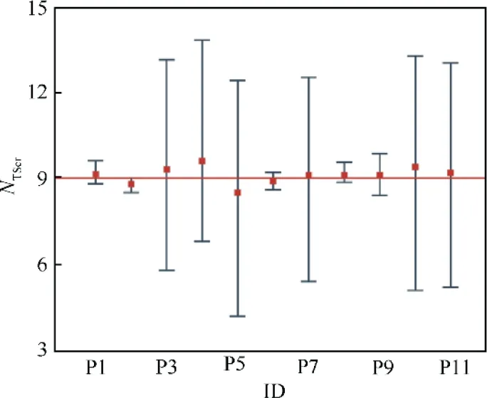
Fig. 1 Business jet wing glove model.

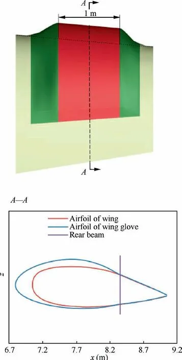
Fig. 2 Geometry and airfoil of wing glove.

The experimental envelope is determined based on the flight test purpose corresponding to a transport aircraft flight regime. The flight matrix is described by Mach number Ma,flight altitude H,and angle of attack α.The pressure coefficient distribution of the test section is changed mainly by adjusting the angle of attack.Fig.3 shows the experimental flight envelope and selected test points.

In Fig. 3, red filled diamond symbols are the selected test points. The chord-based Reynolds number Recis referenced to the chord at the mid-span of the wing glove test section.The Reynolds number Recrange of flight tests is [12.0×106,18.0×106], the Mach number range is [0.46,0.65], and the range of angle of attack is [-0.5◦,2.0◦].

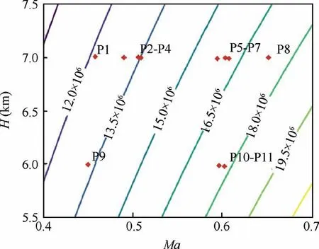
Fig. 3 Flight test points.

2.2. Instrumentation and data acquisition

Both the pressure distribution and the transition location on the upper surface of the wing glove test section are acquired.Pressure distributions are measured through pressure taps.On the upper test section surface, there are two rows of pressure taps distributed along the streamwise direction, and one row of obliquely opened pressure taps, as shown in Fig. 4.Two streamwise distributed pressure taps are labeled as‘‘Sec1”and‘‘Sec2”respectively,and the obliquely distributed pressure taps are labeled as ‘‘Sec3”.

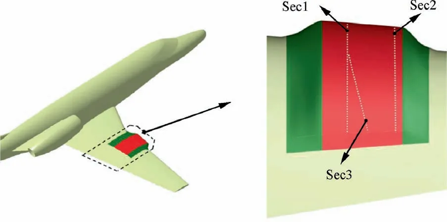
Fig. 4 Pressure measurement with pressure taps.

Transition information is detected by infrared imaging technology. The infrared camera is placed on the fuselage as shown in Fig.5(a).During flight tests,the wing glove is heated by heating wires,installed inside the wing glove,to increase the temperature difference between the test section and the background environment. Due to the different heat exchange coefficients, the laminar flow and turbulent flow show different temperature distributions. In theInfrared (IR) image of Fig. 5 (b), the bright yellow region represents laminar flow,and the other region represents turbulent flow.

The existence of streamwise pressure taps triggers a premature transition from laminar flow to turbulent flow near the leading edge, resulting in turbulent wedges on the surface.Thus, the region between the two turbulent wedges is used for transition detection. Eight equally spaced lines are set on the upper surface of the wing glove in the spanwise direction.These marking lines can help determine the length of the laminar flow extent.

3. Numerical transition prediction method and gradient calculation

3.1. eN method based on linear stability theory

The most widely used transition prediction methods are based on the LST approach. Transition to turbulence is considered as a stability problem subject to disturbances in the laminar boundary-layer flow. For stability analysis, the flow is represented by a steady base flow superimposed with unsteady flow fluctuations, i.e.,

where q is a vector with the velocity components (u, v, w),pressure (p), density (ρ) and temperature (T), q-represents the base flow quantities,and q′represents the fluctuating quantities, which is expanded as

Here,q～denotes the complex amplitude function and it only depends on the flow in the normal direction of the wall boundary. We treat the equations in a temporal framework, so the circular frequency, ω, is a complex number, while a and b are real numbers.

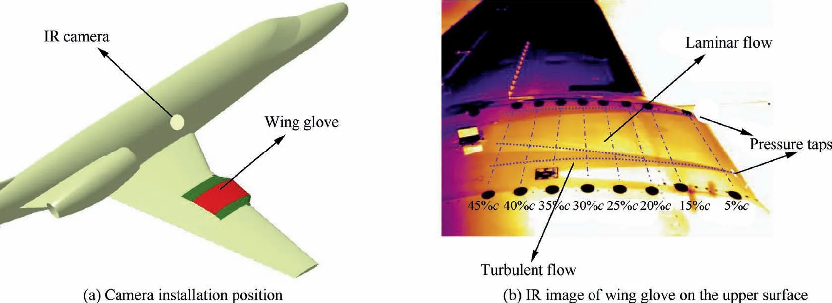
Fig. 5 IR camera installation position and experimental IR image.

By applying Eq. (2) to the Navier–Stokes (NS) equations and neglecting the second-order disturbance terms, we obtain the LST equations with a parallel-flow approximation. The final local stability problem, which is valid for both two- and three-dimensional compressible flows, is expressed as

where C1, C2and C3are determined by the base flow parameters q and the wave numbers a and b. The linear system of ordinary differential equations has been discussed in detail by Cebeci.38

We use a Rayleigh quotient method to efficiently solve the generalized eigenvalue problem of Eq. (3) for the dominant eigenvalue.39Finally, we obtain the imaginary component of the temporal disturbance growth ratio, ωi, which is the imaginary component of the circular frequency. Gaster’s transformation40is used to convert the temporal growth ratio ωiinto the spatial growth ratio ai,which is the imaginary component of wave number.

For the eNmethod, we obtain the N-factor

where ds is arc length in the streamwise direction at the boundary-layer edge and s0is defined as the critical point from which the unstable disturbances start to develop.The N-factor is integrated for different frequencies of the TS wave,or different wavelengths of CF vortices. The maximum value at each chordwise point defines the envelope factor N.When the local envelope factor reaches the critical Ncr, the transition occurs.

3.2. Simplified eN method

Motivated by the need for a fast, robust, and accurate TS waves prediction tool,Drela and Giles23proposed a simplified method–approximate envelope method to replace linear stability analysis to compute the N-factor.In the approximate envelope method, the amplification rates along the envelope of maximum amplification can be linearly approximated for self-similar flows. The envelope amplification factor,NTS, for non-similar flow can be evaluated using

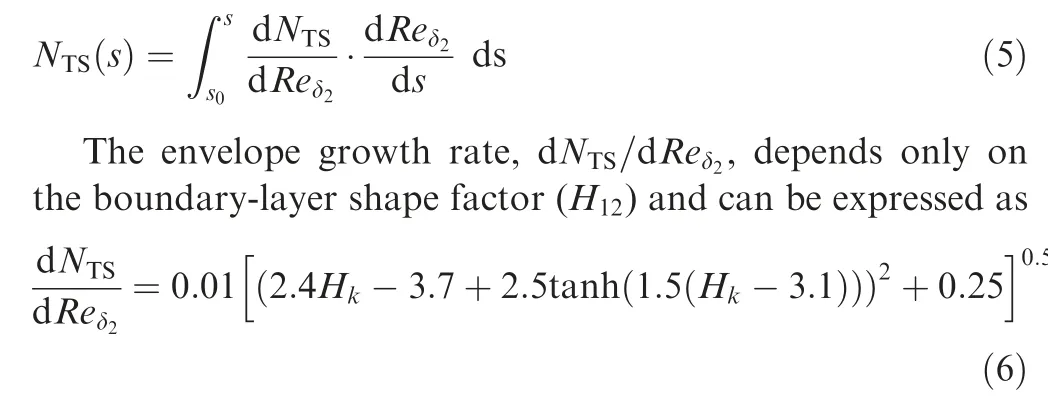
where Hkdepends on the shape factor(H12)and Mach number at boundary-layer edge (Mae) for compressible flow, and is described as

When NTSexceeds the critical value (NTScr), transition caused by TS instabilities occurs.

The boundary-layer information, input of LST, or simplified eNis computed by the laminar boundary-layer equations for quasi-three-dimensional flow with conical assumption.The transition prediction tool coupling RANS solver,boundary-layer code, and LST (or simplified eNmethod),has been described by Shi et al.18,19Since we focus on the low sweep angle tests, the simplified eNmethod is accurate enough to predict TS instabilities.

3.3. Flow solution and verification

Because the wing glove configuration has a small sweep angle at the leading edge, CF instabilities can be ignored. Here, we compare the results of LST based eNmethod and the simplified eNmethod for predicting TS instabilities for a common research model, NLF(1)-0416 airfoil. This airfoil has a thickness ratio t/c=0.16 and is designed to operate at lift coefficient CL=0.4.

We compare the simplified eNmethod results with experimental data for various angle of attack (various CL) at Ma=0.1 and Re=4.0 × 106. According to the relationship of Mack,41NTScris set as 7.2 as the freestream turbulence intensity is 0.15%. We compare the CFD results with experimental data in Fig. 6. The transition locations from CFD results at various angles of attack show an excellent agreement with experimental data,demonstrating the accuracy of the simplified eNmethod for predicting TS instabilities.

For the wing glove experiment, the critical N-factor is calibrated by using LST method.Thus,it is necessary to compare the N-factor obtained by simplified eNmethod and LST method. We show N-factor distribution for both simplified eNmethod and LST method at α=1.5°and CL=0.7 in Fig. 7. Based on our prediction tool, the results of the simplified eNmethod in Section 3.2 are in agreement with the LST results, as shown in Fig. 7, which verifies the accuracy of the simplified eNmethod. The match of N-factor also demonstrates that we can use the critical N-factor calibrated by LST directly when applying the simplified eNmethod in this paper. Note that the N-factor reaches the critical N-factor at the transition point on the lower surface. We also show the results when NTScris 9.0,and the locations of the simplified eNmethod match the results of exact LST.

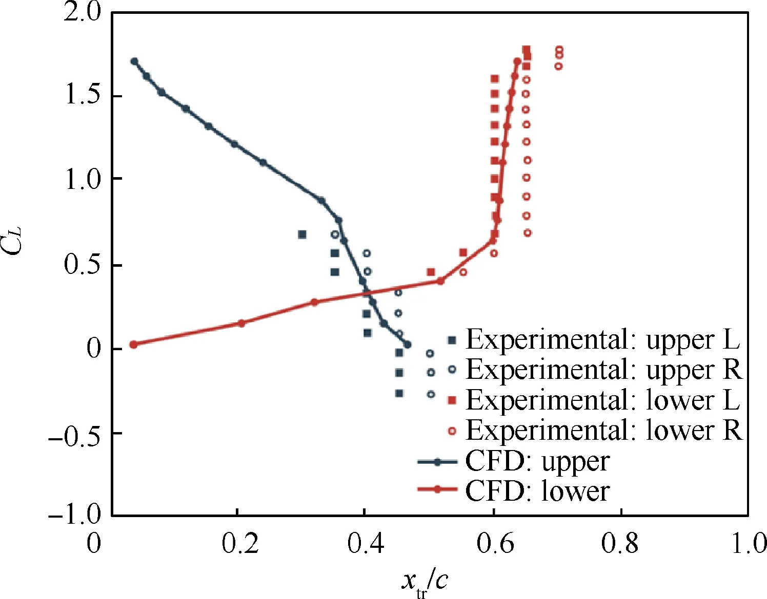
Fig. 6 Comparison of transition location vs CL between CFD and experimental data for NLF(1)-0416 airfoil.

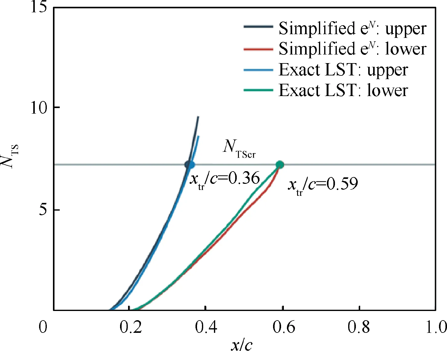
Fig. 7 Comparison of simplified eN method with LST results at α=1.5° and CL =0.9.

3.4. Derivative computation of simplified eN method

We need to compute the sensitivity information of N-factor with respect to base flow parameters, such as Reynolds number and pressure coefficient. The gradient can be computed by the Finite-Difference (FD) method, Complex-Step (CS)approach and Automatic Differentiation (AD) method.

The FD approximations are subject to numerical errors and are not efficient because their cost is proportional to the number of design variables.The CS approach is accurate,but usually makes the code between two and four times slower than the equivalent real code and requires twice as much memory.Furthermore, its cost is also proportional to the number of design variables and requires access to the code, which is not always available.

AD method is another option for computing derivatives accurately. There are two modes for AD: forward and reverse(denoted as an adjoint mode). Both of these modes use the same chain rule, but they accumulate the derivatives in a different direction. We usually use adjoint mode because the number of output variables is typically fewer than the number of input variables for aerodynamic application problems.Considering efficiency,source code transformation is implemented for AD.33

The AD tool is Tapenade.36Firstly,we write the derivative of N-factor at different positions with respect to base flow parameters as forward mode by chain rule

It needs l times for all the streamwise derivatives computation.

Then,the derivative is computed using reverse AD through chain rule,

We need k times to compute all of streamwise derivatives.Since l is larger than k, considering the efficiency, we use the adjoint mode to compute the derivative of N-factor with respect to the base flow parameters.φ-in Eq. (10)can be a unit vector.Using this differentiated function, we can compute individual derivatives by providing the input seed vector of φ-such that the nth entry is one and all other are zeros, i.e.,

For instance,if we compute the derivative of N-factor with respect to Re,the position of φ, which corresponds to Re,has the value of one, and the others are zeros. q is velocity(u, v, w), ρ and T in the boundary layer. In Eqs. (9) and(10),dblconsists of boundary-layer parameters which are integrated by q.dblcan be displacement thickness-based Reynolds number, momentum thickness-based Reynolds number, shape factor, and local Reynolds number, density, Mach number,and viscosity coefficient at the boundary-layer edge.

For a given flow, the vector dblis dependent on

where x is the section coordinates,and bxconsists of Reynolds number, Mach number, turbulence intensity, and critical Nfactor. dblis obtained in boundary-layer code. The first and second term of Eq. (10) are related to the laminar boundarylayer equations, and the third term is computed in the code of simplified eN.Each of the terms utilizes AD tool to compute the derivatives. The laminar boundary-layer code involves non-linear iteration, which requires more efforts to differentiate the source code.

With the verification case (Section 3.3)at α=2°, along the streamwise direction, the derivatives of NTSat x/c=0.2 with respect to Reynolds number and to pressure coefficient are computed. We use the ADjoint method and the FD method.We compare the derivatives of ADjoint method with FD method in Fig. 8, and the AD derivatives match FD results.The selected step size of FD algorithm minimizes the sum of the truncation and subtractive cancellation errors.The derivatives computed with AD method differ from the FD method with relative errors ranging from 10-3to 10-8, which demonstrates the best agreement that can be expected, given the errors inherent in FD approximations.

4. Calibration of critical N-factor with flight test results

We use overset mesh for simulation, as shown in Fig. 9. The first boundary-layer cell height is set to ensure the value of y+below 1. The total number of cells is 5.8 million. A denser mesh is used around the wing glove to ensure the numerical simulation accuracy of the flow field around the wing glove.Tail-mounted layout engines and tails have little impact on the flow physical characteristics under selected flight conditions. Therefore, we simplify the geometry of the business jet by ignoring engines and tails, which will not affect the transition analysis result.

For eNmethods, the critical N-factor is a vital transition criterion for determining a laminar-to-turbulent transition position. The critical N-factor is not a fixed value, which is dependent on the flight test conditions including noise and turbulence intensity, and surface roughness. It is essential to calibrate the critical N-factor of TS waves under flight test conditions for the numerical transition simulation.

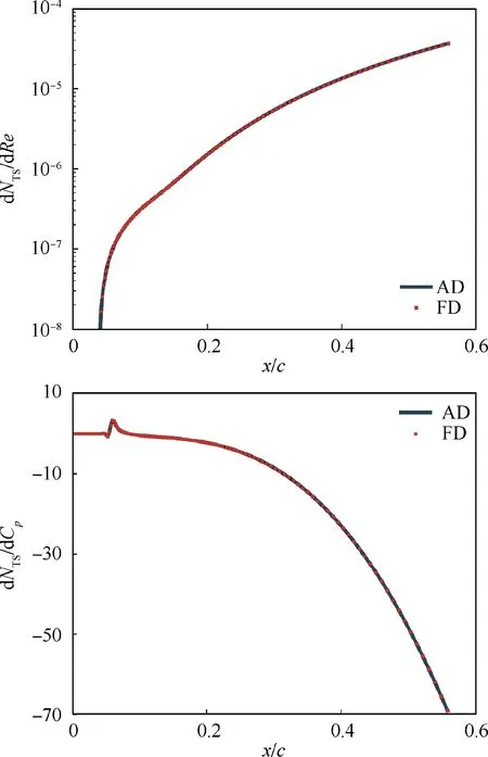
Fig. 8 Comparison of derivative computation between ADjoint method and finite-difference algorithm.

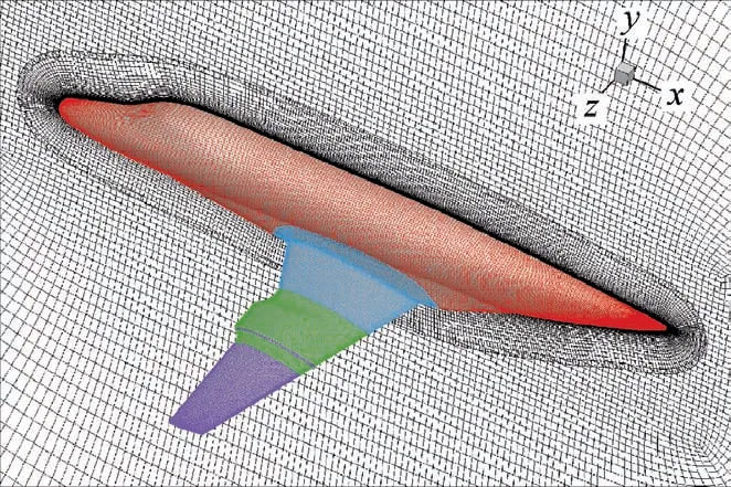
Fig. 9 Overset mesh for CFD calculation.

Based on the LST theory described in Section 3.1,we compute the envelope curve NTSof TS waves on the upper surface of the test section. Combining each enveloped curve in the spanwise direction, we obtain a three-dimensional N-factor contour of the test section, which reveals the development of TS waves (Figs. 10–14). As long as the critical N-factor is determined,the predicted transition line is obtained.IR images show the distribution of laminar and turbulent flow in the form of a temperature field. The statistically best critical Nfactor is obtained by comparing the N-factor contour and IR images.

As shown in Table 1,we select five representative flight test points to illustrate the calibration process of critical N-factor.The most obvious characteristic of the selected data is that the range of flight angle of attack and the chord-based Reynolds number vary widely. These test points can reflect the main impact from pressure distributions and Reynolds numbers.

Figs. 10–14 show numerical results and flight experimental data for the selected flight test points.The data marked by diamond and circle symbols represent the flight test result. The comparison of pressure coefficient distribution in the subfigure(a) of Figs. 10–14 illustrate that the simulation results agree well with the experimental data.There are still some discrepancies,which are mainly due to the geometric difference between the flight model and the simulation model caused by manufacturing and model installation. Note the ’’P3′’ experimental IR image shows possible contamination by insects in the takeoff process, which results in a wedge-shape transition location variation along the spanwise direction.

The subfigures (b) of Figs. 10–14 show the N-factor contours on the clean region for transition detection of the test section. The red line in the subfigures (b) of Figs. 10–14 is the leading edge of the wing glove and the black dotted lines are the positions of pressure taps in the streamwise direction.Black solid lines represent turbulent wedges caused by pressure taps.N-factor contours show different distribution characteristics among the five test points. P1 and P2 have a much larger growth rate of NTS.The value of NTSincreases quickly to more than 10 before 30%c. The rapid growth of NTSmeans an earlier transition.

IR images in subfigures (c) of Figs. 10–11 show that laminar flow extents of P1 and P2 contain around 16%c to 18%c, respectively. The reduction of the favorable pressure gradient and the appearance of the inverse pressure gradient are the main reasons for the rapid increase of NTSnear the leading edge. In comparison, because of large favorable pressure gradients, the growth of NTSat the last three flight test points is much more moderate. The NTSrapid growth only appears in the region with large inverse pressure gradients. IR images show that the maximum laminar flow extent of these three test points is above 45%c.

Another common feature of N-factor contours of all flight test points is that NTSin the region close to the pressure taps section ‘‘Sec1” increases more quickly than the region close to the pressure taps section‘‘Sec2”.A relative larger favorable pressure gradient around ‘‘Sec2” causes such a phenomenon,as shown in the subfigures (a) of Figs. 10–14. IR images also show a similar phenomenon. For instance, Fig. 11 (c) illustrates that the region around ‘‘Sec2” maintains a longer laminar flow extent.

Furthermore, we choose the section at the mid-span of test section as the typical section. For each flight test point, we match the NTScurve of the selected typical section with measured temperature curve to determine the value of critical Nfactor(NTScr),so that the selected section has the same laminar flow extent as flight test results.Through this match,a diagram about N-factor for each flight test point is obtained, as shown in Fig.15.In this figure,points marked with red square are the best match NTScrfor each flight test point.The solid black line at each point represents the 5% transition prediction error band.

Fig. 15 describes the range of critical N-factor that makes sure the transition prediction error below 5%.In the transition prediction 5% error band, the range of critical N-factor for flight test point ‘‘P3” varies widely, reaching as low as 5.8.Among all experimental results, there are six flight test points exhibiting a similar phenomenon. For these points, the transition is triggered in the region(after 40%c)with a large inverse pressure gradient. A large inverse pressure gradient causes a sharp increase in the N-factor(Figs. 10–14),which results in a large value range for the N-factor, and then the wide range of critical N-factor. According to the N-factor distribution, the value of critical N-factor is set to be 9.0, which is marked by a red solid line in Fig. 15.

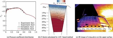
Fig. 10 Transition simulation and flight test results at Ma=0.458, Re=12.22×106, α=2° and H=7.0 km.

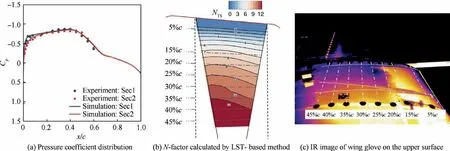
Fig. 11 Transition simulation and flight test results at Ma=0.506, Re=13.51×106, α=1.55° and H=7.0 km.

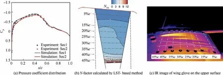
Fig. 12 Transition simulation and flight test results at Ma=0.594, Re=15.85×106, α=0.2° and H=7.0 km.

With the calibrated critical N-factor for TS waves (NTScr),we verify our simplified eNmethod described in Section 3.2.The transition location results of mid-span section for simplified eNmethod simulation are compared with experimental data, as shown in Table 2. The maximum error at different conditions is below 7%,which demonstrates that the simplified eNmethod is accurate under flight test conditions.

5. Sensitivity analysis based on gradient information

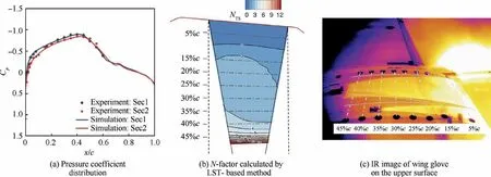
Fig. 13 Transition simulation and flight test results at Ma=0.603, Re=16.09×106, α=-0.15° and H=7.0 km.

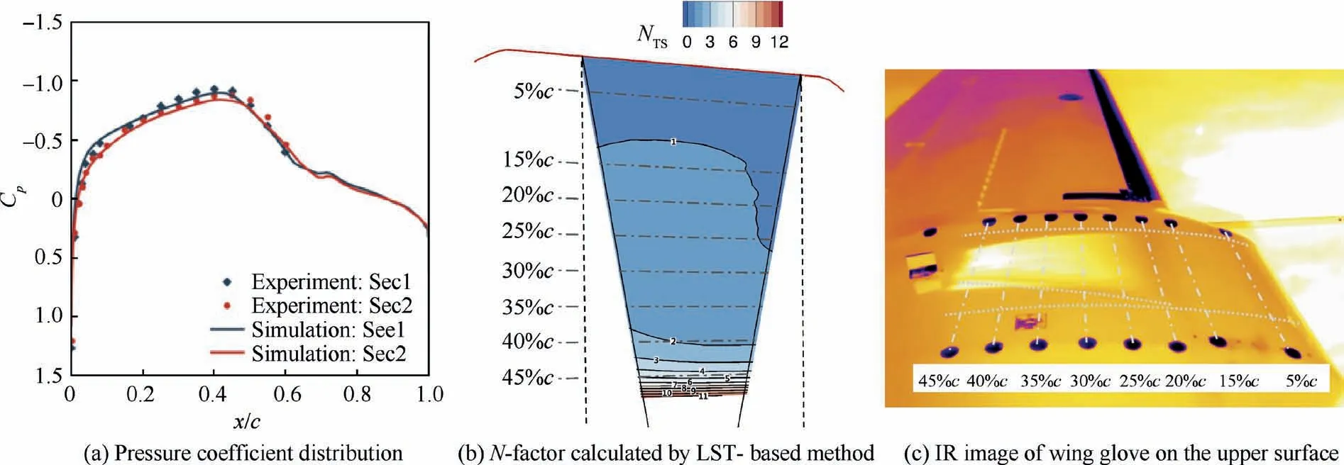
Fig. 14 Transition simulation and flight test results at Ma=0.602, Re=17.86×106, α=-0.3° and H=6.0 km.

Table 1 Representative flight test points.

In this section,the sensitivity analysis based on gradient information is performed to analyze the influence of the Reynolds number (Re)and pressure coefficient (Cp) on the development of TS waves under flight test conditions. We select three test points with different angles of attack and the flight Reynolds number for sensitivity analysis, as shown in Table 3. Among these three test points, ‘‘P4” has the largest favorable pressure gradient and the longest laminar flow extent. A small inverse pressure gradient exists near the leading edge for flight test‘‘P1”,and the laminar flow extent is the smallest.For flight test‘‘P2”, both the magnitude of the favorable pressure gradient and the length of the laminar flow extent are between ‘‘P1”and‘‘P4”.All the simulation and analysis in this section focus on the mid-span test section.

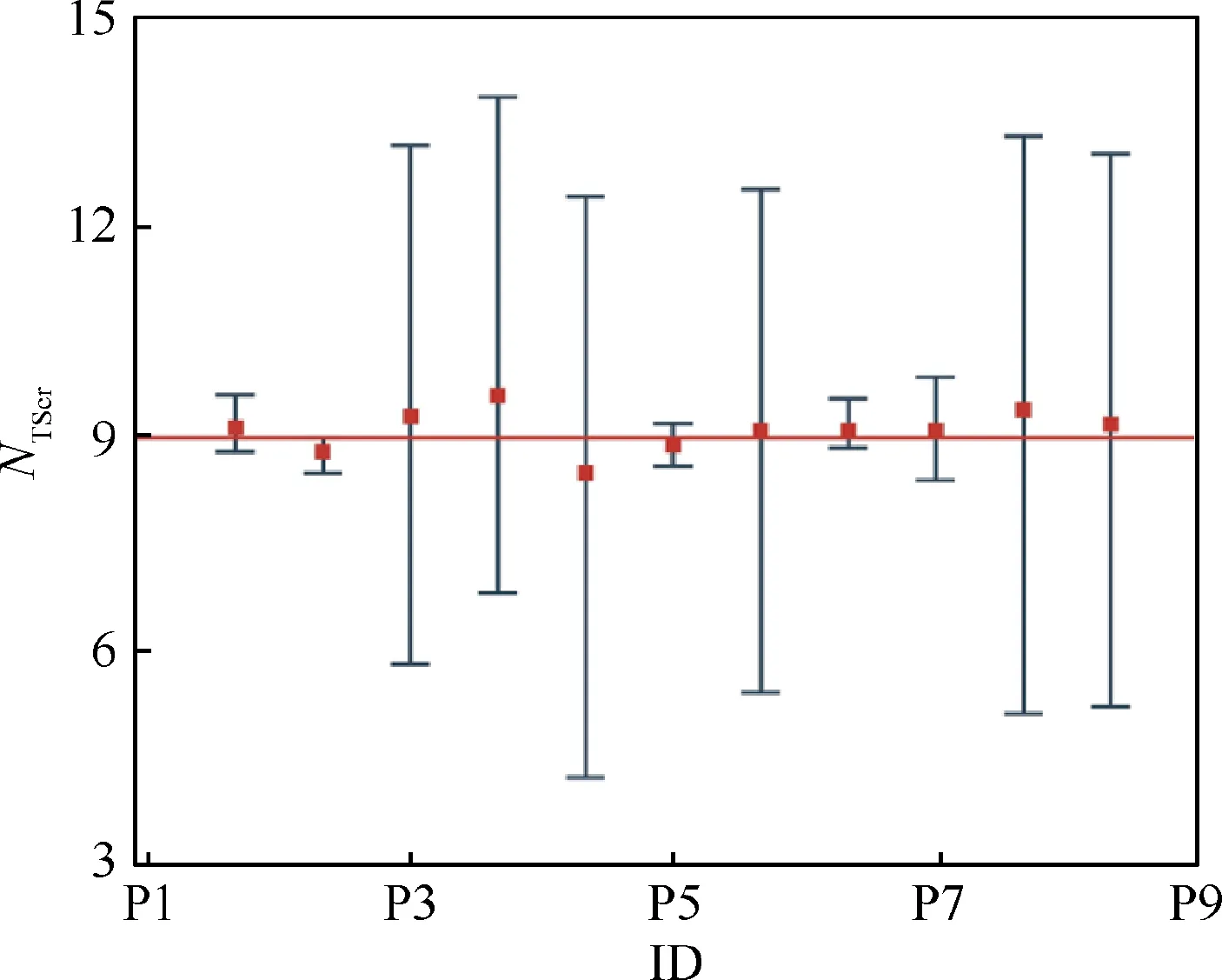
Fig. 15 N-factor diagram for different flight test points.

5.1. Sensitivity analysis of Reynolds number

The distribution of gradients about dNTS/dRecin chord direction is shown in Fig. 16. Fig. 16 (a) shows the comparison of pressure coefficient distributions, and Fig. 16 (b) gives the comparison of dNTS/dRecdistributions in chordwise direction. At different chordwise positions, flight test ‘‘P4” alwayshas the smallest gradient dNTS/dRec. The value of flight test‘‘P2” and ‘‘P1” are close. Lower value of gradients dNTS/dRecindicate higher robustness against Reynolds numbers.

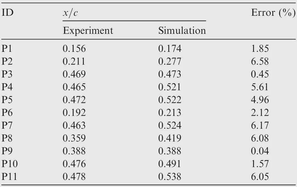
Table 2 Comparison of transition locations between experimental data and simulation results.

Table 3 Representative flight test points.

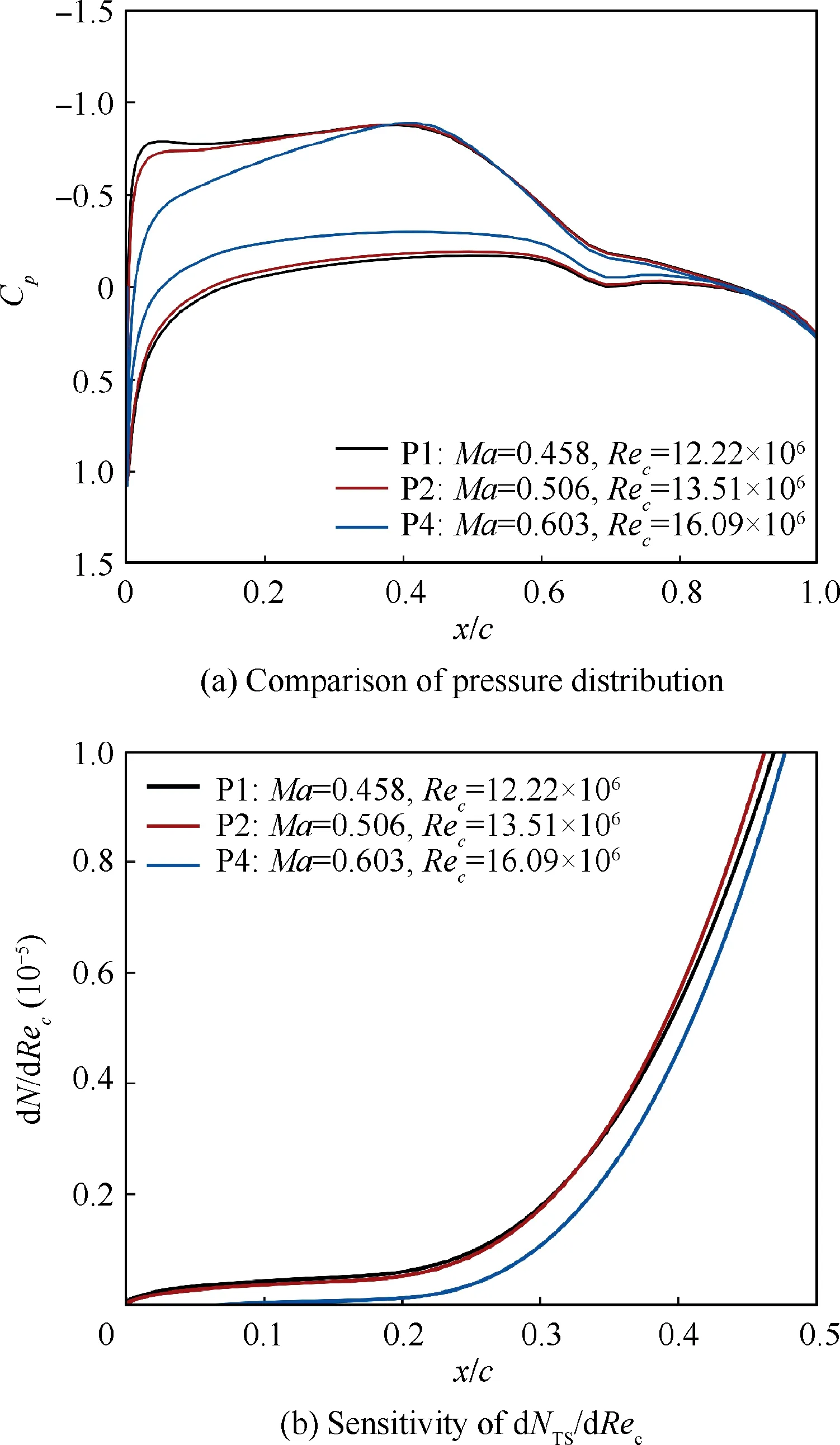
Fig. 16 Comparison of pressure coefficient distribution and sensitivity information (dNTS/dRec) under various conditions.

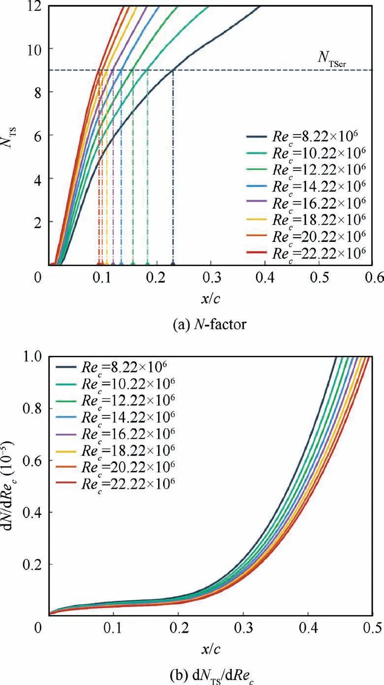
Fig. 17 Comparison of N-factor and sensitivity information dNTS/dRec at different freestream Reynolds numbers for ‘‘P1”.

Based on the distribution of gradient information,dNTS/dRec, the flow development in the chordwise direction shows some obvious features. The part close to the leading edge is a region with small gradient. Because of a large favorable pressure gradient caused by the rapid acceleration of airflow, both dNTS/dRecand its growth rate maintain a low value.

In the region about after 40%c,the gradient dN/dRe maintains a rapid growth with a large growth rate. This region is a pressure recovery area with a large inverse pressure gradient.The envelope curve about the N-factor (Fig. 10(b), Fig. 11(b)and Fig. 13(b)) and the distribution of gradient dNTS/dRecindicate that both the value of NTSand dNTS/dRecincrease rapidly due to inverse pressure gradient.Therefore,the inverse pressure gradient not only accelerates the instability of TS waves(Fig.10(b),Fig.11(b)and Fig.13(b)),but also amplifies the influence of Reynolds number on the development of TS waves.

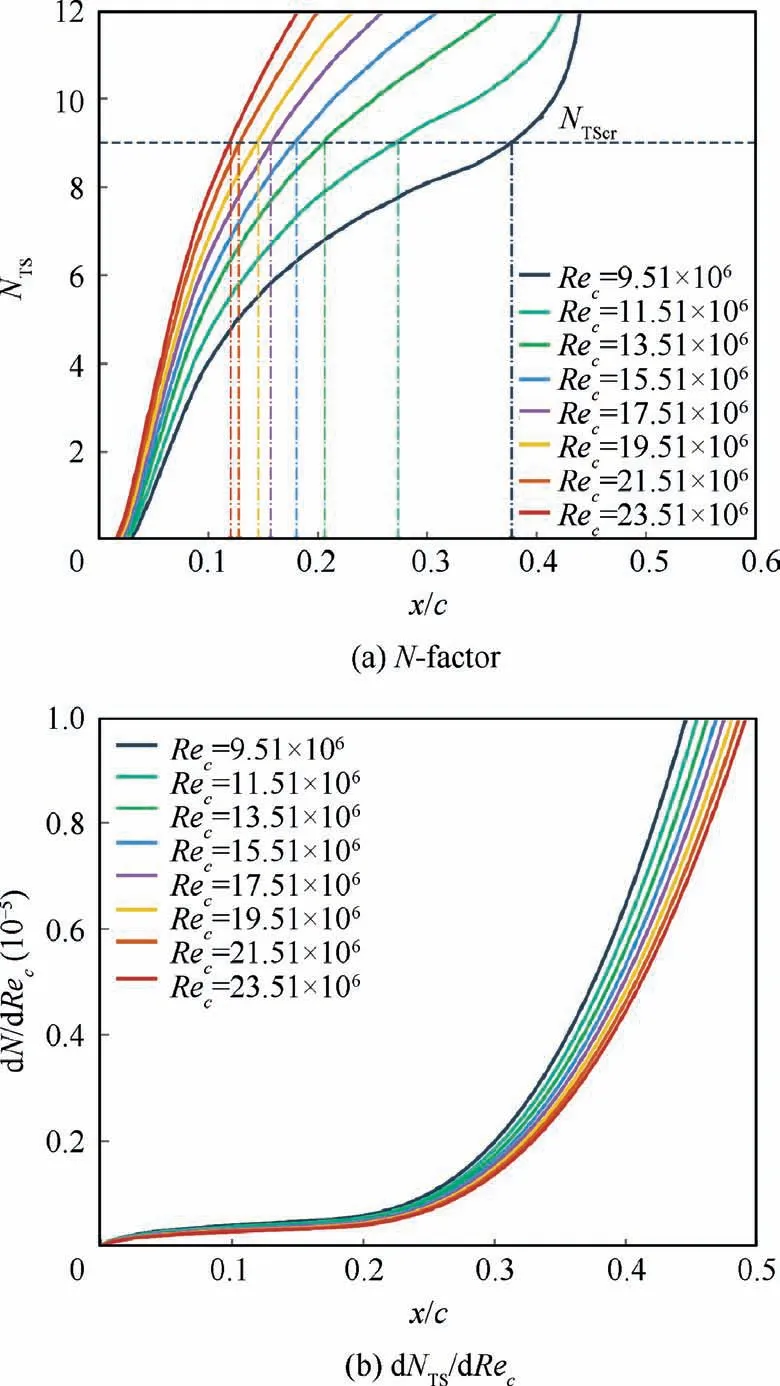
Fig. 18 Comparison of N-factor and sensitivity information dNTS/dRec at different freestream Reynolds numbers for ‘‘P2”.

The middle region before 40%c is an increasing region with relative smaller value compared with the region after 40%c.In this region, the pressure coefficient distribution maintains a favorable pressure gradient, and the value of gradient dNTS/dRecgrows moderately. The growth rate of dNTS/dRecis positively related to the magnitude of the favorable pressure gradient. Fig. 16 demonstrates that because of a large favorable pressure gradient, ‘‘P4” has the smallest gradient of dNTS/dRecin chordwise direction. In conclusion, favorable pressure gradients can help to suppress the development of TS waves and improve the robustness of the transition suppression ability for NLF wings with respect to Reynolds number variation.

Figs. 17–19 show the N-factor (NTS) and gradient dNTS/dRecunder different Reynolds number for these three flight test points. The left figures illustrate the comparison of envelope curve NTSin the range of Reynolds number from 8×106to 24×106. The black dotted lines represent the calibrated critical N-factor, NTScr. Dashed dotted lines label transition locations at different freestream Reynolds numbers.

It can be seen that the flight test ‘‘P4” is the most robust case. When the Reynolds number increases to 23.09×106,more than 45%c laminar flow extent can still be maintained.For flight test point ‘‘P2”, the laminar flow region reduces to about 12%c when the Reynolds number increases to 23.51×106. The performance of flight test ‘‘P1” is the worst.As the Reynolds number increases,the laminar flow transition is triggered quickly just after the leading edge. The transition location is only delayed by about 6%c at Reynolds number of 22.22×106.

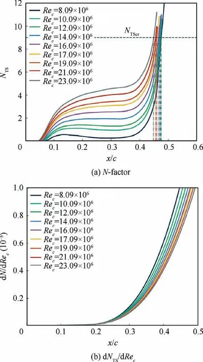
Fig. 19 Comparison of N-factor and sensitivity information dNTS/dRec at different freestream Reynolds numbers for ‘‘P4”.

With the same pressure coefficient distribution, the results show that the higher Reynolds number condition corresponds to a lower gradient value (dN/dRec). This phenomenon is in accordance with the common knowledge of the transition mechanism.42Meanwhile, compared with the analysis of Fig. 16, the influence of Reynolds number on the value of dN/dRecis much smaller than the pressure coefficient.

5.2. Sensitivity analysis of pressure coefficient distribution

The distribution of gradients about dNTS/dCpin chordwise direction is demonstrated in Fig. 20. dNTS/dCpfor each selected flight test point are shown in the form as contour images in the rectangular coordinate system, which is composed of chordwise coordinate positions. The horizontal axis represents the chordwise coordinate of NTS, while the longitudinal axis denotes the chordwise coordinate of the pressure distribution Cp. Therefore, the contour value of point with coordinates xN,xCpis the gradient of NTSat coordinate xNwith respect to Cpat coordinate xCp.

Along the horizontal axis, the slice with the longitudinal coordinate of xNindicates the degree of influence of Cpat each point on NTSat point xN.Correspondingly,along the longitudinal axis, the slice with the horizontal coordinate of x shows the degree of influence of Cpat point xCpon NTSat each point.In order to show the distribution of sensitivity dNTS/dCpmore clearly, an inverse tangent transformation is preformed to adjust the magnitude of dNTS/dCpat each point.

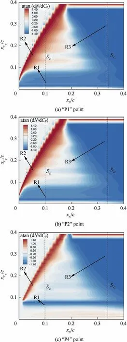
Fig. 20 Sensitivity contour about dNTS/dCp.

Simulation results indicate that there are three regions in which the effect of Cpon NTSis significant. The three regions are marked by ‘‘R1”, ‘‘R2” and ‘‘R3”. The first region, ‘‘R1”,is located near the leading edge before 9%c in the longitudinal axis, and covers the entire area along the horizontal axis. The sensitivity dNTS/dCpin this region is large and negative.Obviously, the pressure coefficient distribution near the leading edge has a significant effect on the development of TS waves for the whole airfoil. Reducing the inverse pressure gradient near the leading edge is one of the most effective ways to reduce NTS.

By comparing the distribution of the region at selected three different flight tests (Fig. 20), we find that the sensitivity value of the region is affected by the local pressure coefficient distribution. In this region, the larger pressure gradient leads to a smaller sensitivity value. Since flight test ‘‘P4” maintains a large favorable pressure gradient in the area before 6%c(Fig.20(c)),only the narrow area of 6%c-9%c in the longitudinal direction has large negative sensitivity value.

The second region, ‘‘R2”, appears as a long narrow strip with a large positive sensitivity value, which is mainly marked by red color.For all selected three flight test points,the region is distributed before 20%c in the horizontal axis direction.Therefore, only NTSof the area before 20%c is significantly affected by the pressure coefficient disturbance in this region.We take longitudinal slice Sv1at xN= 0.1c as an example to illustrate the influence of the pressure coefficient disturbance at each point on NTSin the area before 20%c. It can be seen from Fig. 20 that, along the slice Sv1, the position with large sensitivity value in region ‘‘R2” is behind the position whose value of NTSis cared.

Sensitivity results show that a decrease of pressure coefficient in region ‘‘R2” can effectively suppress the development of TS waves before the region. The transition suppression mechanism of the pressure coefficient disturbance in region‘‘R2”is that the reduction of pressure coefficient in this region can significantly increase the size of the favorable pressure gradient. Similar to the results of region ‘‘R1”, the size of region‘‘R2” with large positive sensitivity is affected by local favorable pressure gradient. A large favorable pressure gradient can narrow the region with large positive sensitivity (Fig. 20(c)), reducing the sensitivity of the TS waves with respect to pressure coefficient.

In region ”R3′′, the area before 37%c maintains large negative sensitivity values. But, after 37%c, the gradient dNTS/dCpincreases rapidly to a high value just around 40%c for these three flight test points.The rapid increase of the gradient dNTS/dCparound 40%c is due to the fact that the favorable pressure gradient reduces quickly and translates to a large negative pressure gradient finally, as shown in Fig. 10,Fig. 11 and Fig.13.Thus,another effective way to suppress the development of TS waves is to increase the favorable pressure gradient by reducing the pressure coefficient around 40%c.

6. Conclusions

We conducted flight experiments and numerical analysis to research the design concept of natural laminar flow wing under the operational conditions of a typical transport aircraft.

We performed flight tests based on a wing glove configuration to advance the natural laminar flow control wing concept and to provide high-quality data for evaluating the physical processes associated with the TS transition mechanism. Flight test results show that maintaining favorable pressure gradients is the key to delay transition and to improve the robustness of natural laminar flow wings under flight conditions with high Reynolds numbers. It is found that, at Reynolds number of 17.8×106, the laminar flow extent is up to 47%c.

The critical N-factor used as transition criterion was calibrated to be 9.0 with flight test data and linear stability theory from a statistical point of view,which makes sure that the transition prediction relative error is below 5%. The calibrated critical N-factor for eN-based method under flight conditions for a typical transport aircraft enriched the data in the field of transition prediction research based on eNmethod.

Considering efficiency, a reliable simplified eNtransition numerical prediction method was implemented,which can capture the TS waves induced transition and has a similar transition prediction accuracy with the linear stability theory.Then,we developed an ADjoint method for derivatives computation of the simplified eN. A good agreement with finite-difference derivative approximations was demonstrated for the AD methods.In most cases,the derivatives computed by both methods match with each other for four digits or more. Thus, the efficient AD method is demonstrated to be accurate as well.

We studied the influence of Reynolds numbers and pressure distributions on TS waves by analyzing the sensitivity information computed by AD method. From the Reynolds numberbased sensitivity analysis results, we conclude that a favorable pressure gradient not only suppresses the development of TS waves in the chordwise direction but also decreases the sensitivity of Reynolds number to the development of TS waves.Thus, a favorable pressure gradient would ultimately improve the robustness of transition suppression for natural laminar flow wings. Meanwhile, from the sensitivity analysis results of pressure coefficient distribution on TS waves,we found that maintaining an appropriate pressure gradient is one of the main mechanism for suppressing the development of TS waves. We found three regions in which the pressure distribution disturbance had a significant impact on the development of TS waves at different chordwise positions. Additionally,the sensitivity decreased as the local favorable pressure gradient increased. The conclusion drawn from sensitivity analysis can provide valuable information for the development of robust natural laminar flow wings from the perspective of robustly maintaining laminar flow.

Declaration of Competing Interest

The authors declare that they have no known competing financial interests or personal relationships that could have appeared to influence the work reported in this paper.

Acknowledgement

This work was supported by the National Natural Science Foundation of China (No. 12002284).