Sequential ensemble optimization based on general surrogate model prediction variance and its application on engine acceleration schedule design

Yifan YE, Zhanxue WANG, Xiaobo ZHANG

Shannxi Key Laboratory of Internal Aerodynamic in Aero-Engine, School of Power and Energy, Northwestern Polytechnical University, Xi’an 710072, China

KEYWORDS

Abstract The Efficient Global Optimization(EGO)algorithm has been widely used in the numerical design optimization of engineering systems. However, the need for an uncertainty estimator limits the selection of a surrogate model. In this paper, a Sequential Ensemble Optimization(SEO) algorithm based on the ensemble model is proposed. In the proposed algorithm, there is no limitation on the selection of an individual surrogate model.Specifically,the SEO is built based on the EGO by extending the EGO algorithm so that it can be used in combination with the ensemble model. Also, a new uncertainty estimator for any surrogate model named the General Uncertainty Estimator (GUE) is proposed. The performance of the proposed SEO algorithm is verified by the simulations using ten well-known mathematical functions with varying dimensions. The results show that the proposed SEO algorithm performs better than the traditional EGO algorithm in terms of both the final optimization results and the convergence rate.Further,the proposed algorithm is applied to the global optimization control for turbo-fan engine acceleration schedule design.

1. Introduction

High-fidelity computer simulations play an essential role in the investigation of modern aerospace engineering systems. However, the computational cost of the computer simulations is still excessive even when the highly-developed computer technology is used, especially for the numerical design optimization of engineering systems. The computational cost can be reduced by using the Surrogate-Based Optimization (SBO) in the investigation of the design optimization of aerospace engineering systems.

Efficient Global Optimization (EGO)1is a popular SBO algorithm. The EGO and its other versions have been widely used in the investigation of modern aerospace engineering systems. Jones et al.1proposed an EGO based on the Kriging model, where the new sample points were added using the Expected Improvement (EI) infill criterion2, and the real response was regarded as a normally distributed random variable with the mean and standard deviation given by the Kriging model predictor and its standard error.The point with the maximum EI was added in the sample points to update the surrogate model.The EGO and its other versions have been widely used in the design optimization of complex engineering systems.

Wang et al.3extended the EI and put forward a modified sequential Kriging optimization method to save the time consumption of the sequential Kriging optimization process.Zhang et al.4constructed a double-stage metamodel that integrates the advantages of both the interpolation metamodel and the regression metamodel. Im and Park5proposed a method that combines the particle swarm optimization, surrogate models,and Bayesian statistics to solve structural optimization problems. Jiang et al.6established an integration design method of aerodynamic/stealth for helicopter rotor based on the surrogate model optimization technique. Chao et al.7utilized the low-fidelity model and the multi-infill strategy in a computationally efficient optimization method for aerodynamic design. Li and Pan8proposed a trust region method for the framework of an SBO process based on the Kriging model to accelerate the convergence rate and improve the local exploitation ability. Han et al.9proposed a variable-fidelity optimization algorithm with application to the aerodynamic design.In their work,a multi-level hierarchical Kriging model was referred to as a surrogate model that could incorporate simulation data with an arbitrary fidelity levels.Bu et al.10used the hierarchical Kriging model for rotor design optimization to improve the efficiency of the traditional Kriging model.

The accuracy and robustness of the surrogate model used in the SBO affect the SBO algorithm performance. Various surrogate models have been used in the investigation of engineering design, including the Polynomial Response Surface(PRS)11, Radial Basis Function (RBF)12, Kriging (KRG)13,Gaussian Process(GP)14,neural networks15and Support Vector Regression (SVR)16. The related research has proven that the performance of an individual surrogate model is relatively different for the different design problems. Simpson17and Jin18et al. provided recommendations on the selection of surrogates for different problems by comparing various surrogate models. However, the behavior of an individual surrogate is generally unknown in advance, but building an ensemble of surrogates is an efficient method to enhance the accuracy and robustness of the surrogate model.

The ensemble of surrogate models can be roughly categorized into the average ensemble models and the pointwise ensemble models. The weights of the average ensemble model stay constant over the entire design space,while the weights of the pointwise ensemble models change with the prediction point. Many researchers proposed different ensemble models and proved that the ensemble models showed better performance than the individual surrogate models in terms of both accuracy and robustness. Goel et al.19proposed an average ensemble of surrogates and noted that the variance in the prediction of multiple surrogate models is large in the regions with large uncertainty.Viana et al.20proposed an average ensemble of surrogates based on the minimization of the Mean Square Error (MSE). Acar21proposed five different pointwise ensemble models and compared their performances. Zhou et al.22proposed a recursive process to build an average ensemble model. Lee and Choi23calculated the weight factors at the observed points by using the local error measure of several nearest observed points. Liu et al.24presented an optimal weighted pointwise ensemble by using a new local error measure. Chen et al.25divided the design space into two parts,and global and local error measures were introduced to evaluate the weight factors in these two parts. Ye et al.26built a pointwise ensemble model by using the local error measure of the region near the observed points.

All recent investigations on the ensemble model have shown that the ensemble model have better performance than the individual surrogate models in terms of both accuracy and robustness. The ensemble models have been widely applied to the investigation and design of modern complex engineering. Samad and Kim27used multiple surrogate models including the PRS, KRG, radial basis neural network, and a weighted average ensemble of surrogates in a compressor blade shape optimization. They found that the most accurate surrogate did not always lead to the best design, and even though the weighted surrogate model was not the best in any case, it provided satisfactory results in most cases and protected against choosing a poor surrogate.Glaz et al.28also used multiple surrogate models,including a weighted average ensemble of surrogates for the rotor blade vibration-reduction problem.They also found that the most accurate individual surrogate model might not lead to the best design. In addition, designs obtained by using multiple surrogate models performed better than the designs obtained by using a single surrogate model.

The EGO performance can be further improved by building the ensemble model with different types of individual surrogate models, such as RBF and PRS. In the traditional EGO algorithm, the EI infill criterion is used to generate new sample points. This infill criterion is constructed by using the surrogate prediction value and prediction uncertainty. The Kriging model used in the traditional EGO algorithm can provide the uncertainty estimator. However, many surrogate models cannot provide this uncertainty estimator. Thus, the need for the surrogate uncertainty estimator limits the selection of the surrogate model in EGO. There are also multiple kernel techniques that can be used for building the Kriging model. Ginsbourger et al.29suggested combining the Kriging model with multiple kernel functions to assist the EGO. Palar and Shimoyama30investigated using multiple kernel functions for assisting the single-objective Kriging-based efficient global optimization. Since all the constituent surrogate models in the ensemble scheme were Kriging models, it performed the EGO since the Kriging uncertainty structure was still preserved. However, this technique also limits the selection of individual surrogate models.

Motived by these findings, the authors propose a General Uncertainty Estimator (GUE) that can provide the prediction variance measure for any surrogate model. Also, a Sequential Ensemble Optimization (SEO) algorithm is built based on the work by Jones et al.1in extending the EGO algorithm so that it can be used based on the ensemble model that is constructed by any type and number of individual surrogate models.

With the goal to reveal the relationship between the performance of the SBO with the surrogate model and uncertainty estimator,the performances of SEO based on different existed ensemble models are compared first, and then the performances of SEO based on the ensemble model and its individual surrogate models are compared. The performances of the GUE and Kriging uncertainty estimator are also compared.Further, the SEO is employed in the global optimization control for turbo-fan engine acceleration schedule design.

2. Sequential ensemble optimization algorithm

As mentioned above, the proposed SEO algorithm is developed based on the work by Jones et al.1in extending the EGO algorithm so that it can be used based on the ensemble model that is constructed by any type and number of individual surrogate models. In the EGO, the surrogate uncertainty estimator of the Kriging model is used to select the next sampling candidate.However,many surrogate models do not provide this uncertainty estimator. Therefore, the need for the surrogate uncertainty estimator limits the selection of a surrogate models in the EGO.

In this paper, GUE is proposed to provide a prediction variance measure for any individual surrogate model and ensemble model with any type and number of individual surrogate models,and the ensemble model is employed in the EGO.

2.1. General uncertainty estimator

The pointwise cross-validation error represents a data-based error measure, and it can provide a global or local error measure for any surrogate model. It has been widely used as the surrogate error measure to build the ensemble model.

Thus, this paper construct the surrogate model prediction variance by using the pointwise cross-validation error. However, the pointwise cross-validation cannot be used directly as the surrogate model uncertainty estimator due to two major factors responsible for such difficulty.

Firstly, the pointwise cross-validation error is discrete and has a value different from zero at the observed point.However,the prediction variance is continuous and the prediction variance at the observed points is zero. Also as the distance from the observed points increases,the prediction variance increases.

Secondly, the pointwise cross-validation error at a single observed point cannot reflect the surrogate model’s local error in the region around the observed point.Acar21has noted that pointwise cross-validation error is not a good surrogate for the error at a point.However,some researchers,including Lee and Choi23and Ye et al.26, used the pointwise cross-validation error at multiple observed points as error criteria in the region around the observed points.Therefore,in this work,the surrogate model prediction variance is constructed by using the cross-validation error at multiple observed points.

First, the local prediction variance of the region around each observed point is obtained by using the cross-validation error at multiple observed points, and then, the continuous global surrogate prediction variance is obtained by combining all local prediction variances.

The local prediction variance of the region around the observed point xiis calculated by:where videnotes the local prediction variance of the region around the observed point xi, n denotes the number of observed points, eXVjrepresents the pointwise crossvalidation error of the surrogate model at the jthobserved point, and dj(x) denotes the distance between x and the jthobserved point.

A one dimensional example of the local prediction variance curve of the region around the observed point A is presented in Fig.1,where X denotes the model input,Y denotes the prediction variance, the black dots denote the cross-validation error at three observed points A,B,and C,and the red curve denotes the local prediction variance of the region around the observed point A. The part of the curve near the observed point A is used to construct the surrogate global prediction variance.As shown in Fig.1,the local prediction variance is continuous,and the local prediction variance at observed point A is zero.Besides, as the distance from observed point A increases, the prediction variance also increases.

The continuous global surrogate prediction variance is constructed by combining all local prediction variance as:

where v denotes the global surrogate prediction variance, and videnotes the local prediction variance of the region around the observed point xi.

A one dimensional example of the global and local prediction variance curve of the region around the observed points are presented in Fig. 2, where X denotes the model input,and Y denotes the prediction variance. The design space can be divide into several hyper-volumes. In each hyper-volume,there is a local prediction variance that is smaller than the other local prediction variance. At the hyper-volume boundary,there are two or more local prediction variances that have the same value. In the hyper-volume, the global prediction variance is the same as the local prediction variance that is smaller than the other local prediction variance in that hyper-volume, thus the global prediction variance is continuous in the hyper-volume. At the hyper-volume boundary, the global prediction variance has the same value on the boundary, so the global prediction variance is continuous on the hyper-volume boundary. From the hyper-volume boundary to any hyper-volume, the global prediction variance is the same as the local prediction variance that is smaller than the other local prediction variance in that hyper-volume.Thus,the global prediction variance is continuous in the whole design space.

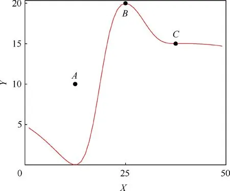
Fig. 1 Curve of local prediction variance of the region around the observed point A.

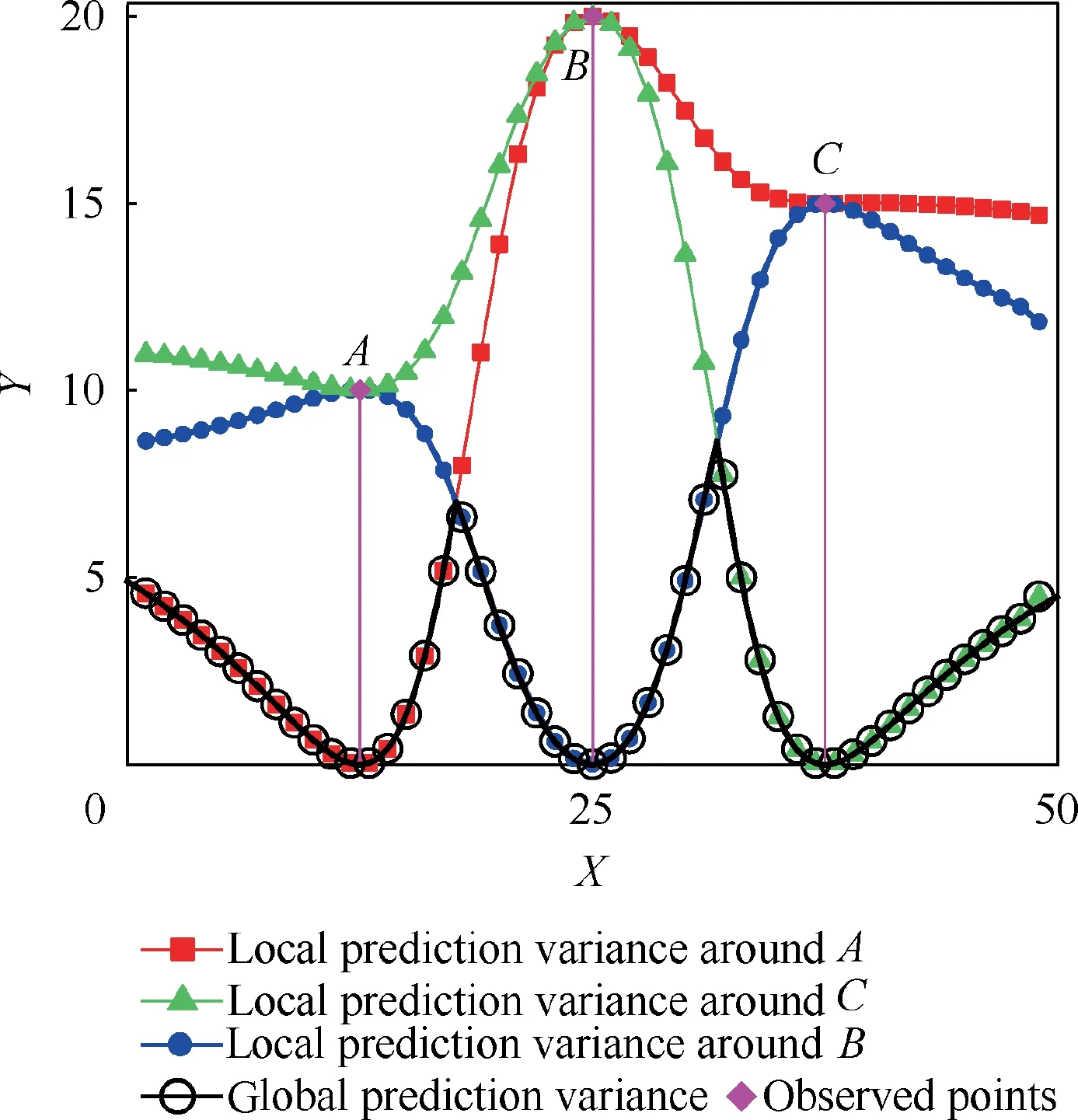
Fig. 2 Global and local prediction variance curves of region around observed points.

As shown in Fig.2,the general surrogate model uncertainty estimator can reasonably reflect the surrogate prediction variance. First, the prediction variance at the observed point is zero, and as the distance from the observed points increases,the prediction variance also increases. In addition, the crossvalidation error of point C is larger than that of point A.Thus,the prediction variance of the region between points B and C is larger than that of the region between points B and A.

2.2. SEO algorithm framework

The flow chart of the traditional EGO algorithm and the proposed SEO algorithm are shown in Figs. 3 and 4 respectively.

The construction of the traditional EGO algorithm includes five following steps:

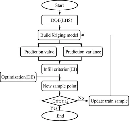
Fig. 3 Flow-chart of traditional EGO algorithm.

(1) Generation of the initial sample points using the Design of Experiments (DOE) and the calculation of the corresponding responses.

(2) Construction of the Kriging model based on the current sample points and their responses.

(3) Determination of the Kriging model prediction value and corresponding prediction variance.

(4) Calculation of the surrogate model EI (an infill criterion) using the prediction value and prediction variance of the Kriging model.

In the EGO algorithm, the real response is regarded as a normally distributed random variable Y(x) with the mean and standard deviation given by the Kriging model prediction value and its prediction variance. Thus, the improvement at a point x is defined as

where ybestdenotes the currently best sample, y’ denotes the prediction value of the Kriging model at point x, and v(x)denotes the Kriging model prediction variance at point x, N denotes the normally distributed random function. The EI is defined as:

where u denotes the standard error that the value of the currently best sample is above the prediction value of the Kriging model at point×,Φ(⋅)and φ(⋅)denotes the cumulative density function and the probability density function of a normal distribution, respectively.

(5) Generation of a new sample point based on minimization of the EI. The Differential Evolution (DE) algorithm is used in this paper.

(6) Rebuilding of the Kriging model until the termination criterion is satisfied.

As previously mentioned, in the EGO algorithm, the need for an uncertainty estimator limits the selection of a surrogate models. As presented in Section 2.1, the proposed GUE can provide an uncertainty estimator for any surrogate model.Thus, the SEO is built based on the EGO by extending the EGO algorithm so that it can be used based on the ensemble model that is constructed by any type and number of individual surrogate models.

The construction of the proposed SEO includes nine main steps, which are given in the following:

(1) Generation of the initial sample points using the DOE and the calculation of the corresponding responses.

(2) Construction of the individual surrogate models based on the current sample points and their responses.In this paper, the RBF, KRG, and PRS surrogate models are selected.

where yidenotes the real response at the ithobserved point,and y-i’ denotes the corresponding predicted value from the individual surrogate constructed by using all the observed points except the ithobserved points.

(4) Development of the individual surrogate model weight factors using the cross-validation error, and construction of the ensemble model by combining different individual surrogates into a weighted-sum formulation as follows:

where ye’denotes the predicted value obtained by the ensemble model, and yj’ denotes the predicted value obtained by the jthindividual surrogate model,and wjis the corresponding weight factors of the jthindividual surrogate model,and m denotes the number of individual surrogate models.

In this paper, four different ensemble models are selected.The ensemble model based on the heuristic method by Goel et al.19is labeled as EG,the OWSdiag model by Viana et al.20is labeled as Od,and two spatial models by Acar21are labeled as SP1 and SP2, respectively.

(5) Calculation of the pointwise cross-validation error of the ensemble model using the pointwise crossvalidation error and weight factors of each individual surrogate. In order to reduce the time consumption of rebuilding the ensemble model, the pointwise crossvalidation error of the ensemble model is calculated by:

where eXVedenotes the pointwise cross-validation error of the ensemble model, and eXVjdenotes the pointwise crossvalidation error of the jthindividual surrogate model, and wjrepresents the weight factors of the jthindividual surrogate model, and m denotes the number of individual surrogate models.

(6) Determination of the ensemble model prediction variance using the cross-validation error of the ensemble model. This step has already been described in Section 2.1.

Next day he was led before the Emperor, who at once condemned10 him to death and to be thrown into a dark dungeon11 till the day of his execution arrived

(7) Calculation of the ensemble model EI using the prediction value and prediction variance of the ensemble model. And the DE is selected in this paper.

(8) Rebuilding of the individual surrogate model until the termination criterion is satisfied.

2.3. Research questions

In order to reveal the relationship between the SBO performance and the surrogate model and uncertainty estimator,several specific questions are considered.

2.3.1. Effect of ensemble model on SEO performance

The proposed SEO represents a sequential ensemble optimization algorithm based on the EGO. First, the performances of the EGO and SEO are compared. In order to investigate further the effect of the ensemble model on the SEO performance,four SEO algorithms based on different ensemble models are compared with the traditional EGO. The setup parameters of the SEO and EGO algorithms are given in Table 1.

In the EGO algorithm, the Kriging model with constant trend model and Gaussian correlation function is used. In all SBO algorithms, the EI criterion is used to generate new sample points, and one new sampling point is generated per optimization cycle. The details of individual surrogates that are used to build the ensemble model in the SEO are shown in Table 2. Three RBF models, two KRG models, and a PRS model are considered in this paper. Three RBF surrogates are based on the Inverse Multi-Quadric (IMQ) formulation,Thin-Plate Spline(TPS)formulation,and Gaussian(G)formulation with the constant c=1. As for the Kriging models,both the constant trend model, KRG0, and the linear trend model KRG1 are used, and a Gaussian correlation function is utilized.The PRS surrogate is represented by the fully quadratic polynomial.

2.3.2.Effect of individual surrogate model on SEO performance.

Many investigations on the ensemble model show that the accuracy of the ensemble model is usually slightly worse than that of the most accurate individual surrogate model. However, some studies show that the performance of the surrogate-based optimization based on the ensemble model is better than that based on the most accurate individual surrogate model. Therefore, the performance of the SEO based on the ensemble model and different individual surrogate models shown in Table 2.

2.3.3. Effect of uncertainty estimator model on the SEO performance.This paper proposes a GUE to provide an uncertainty estimator for any individual surrogate model.The Kriging model prediction variance can also be used to provide an uncertainty estimator for the other individual surrogate model and ensemble model.Thus,the cases where different surrogate models are used for function prediction and the KrigingUncertainty Estimator (KUE) is used for EI estimation are analyzed.

Table 1 Setup parameters of the SEO and EGO algorithm.

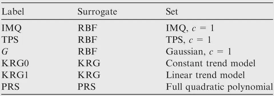
Table 2 Individual surrogate models used in SEO.

3. Simulation procedure

3.1. Benchmark problems

In order to verify the performance of the proposed sequential optimization method, ten well-known example problems with dimensions varying from two to twelve were considered. The parameters of the analytic test problems are presented in Table 3.

In all the test problems, the Latin Hypercube Sampling(LHS) technique was adopted to generate the initial sample points. The initial sample points were generated using the MATLAB routine ‘‘lhsdesign” and ‘‘maximin” criterion with the maximum iteration number of 1000. In order to eliminate the influence of the initial data set, the experiments were conducted with 100 different LHS for low dimension problems(Branin-Hoo, Camelback, Glodstein-Price, and Cross-INTRAY), and the number of initial datasets was reduced as the number of dimensions is increased.

The number of initial sample points of each test function was set to be six times the dimension of the test problems.The maximum number of optimization cycles was 18 and 12 times the dimension of the test problems for the lowdimension problems and high-dimension problems, respectively. The number of the initial sample points for the Sphere text function was 72, and the number of the initial sample points for the Dixon-Price text function was 92. This was because there was a low limit on the number of sample points for the fully quadratic polynomial PRS, which was used as an individual surrogate in the numerical procedure.

(1). Branin-Hoo function (two variables):

where x1∊[-5,10] and x2∊[0,15].

(2). Camelback function (two variables):

Table 3 Parameters of test problems.

where x1∊[-3,3] and x2∊[-2,2].

(3). Glodstein-Price function (two variables):

where x1, x2∊[-2,2].

(4). Cross-IN-TRAY function (two variables):

where x1, x2∊[-6,6].

(5). Hartman function (three variables):

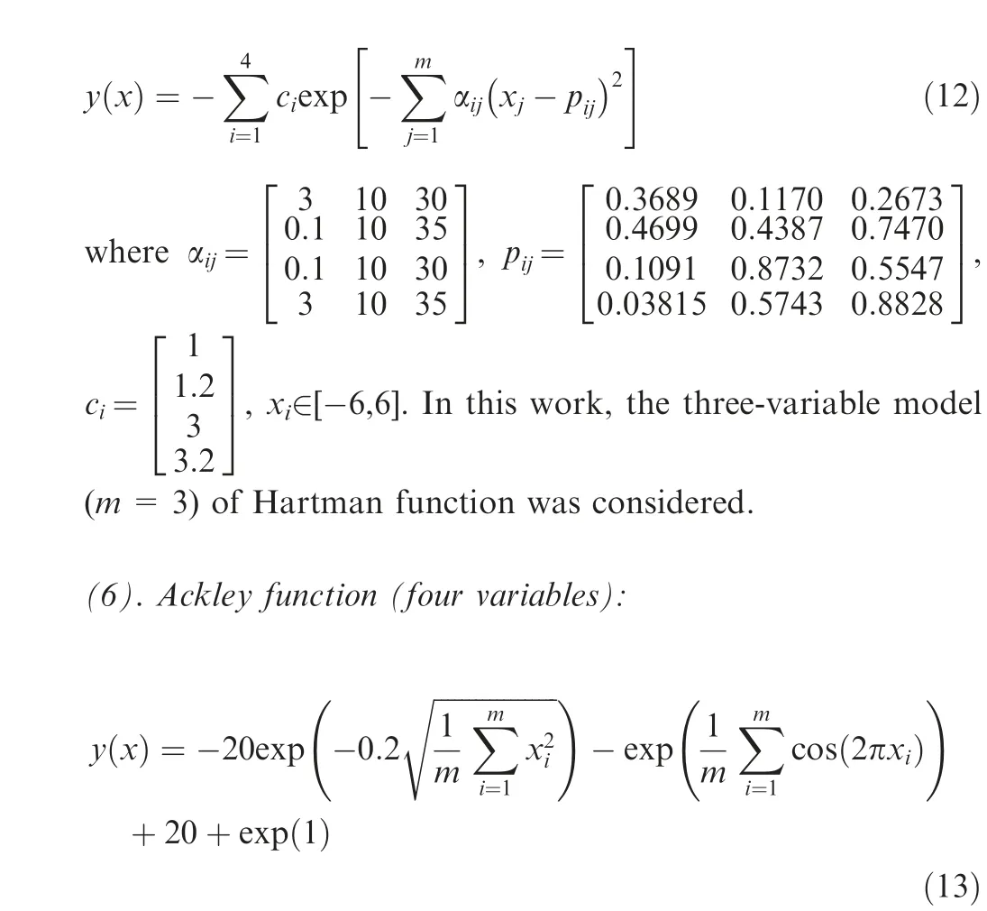
where xi∊[-2,2].In this work,the four-variable model(m=4)of Ackley function was considered.

(7). Colville function (four variables):

(8). Extended Rosenbrock function (eight variables):

where xi∊[-5,10]. In this work, the eight-variable model(m=8) of extended Rosenbrock function was considered.

(9). Sphere function (ten variables):

where xi∊[-5.12,5.12]. In this work, the ten-variable model(m=10) of Sphere function was considered.

(10). Dixon-Price function (twelve variables):

where xi∊[-10,10]. In this work, the 12-variable model(m=12) of Dixon-Price function was considered.

3.2.Global optimization control of turbo-fan engine acceleration schedule design

In order to validate the proposed algorithm in the engineering application, a global optimization acceleration control of a mixed-flow turbo-fan engine was considered. The control schedule of fuel flow(Wf)was selected as the optimization variables, and the control schedule was altered to the Bezier curves31. The engine simulation model was formed using the aero-engine simulation system proposed by Zhang et al.32,and it is presented in Fig. 5.

Fig. 5 Mixed-flow turbo-fan engine model.

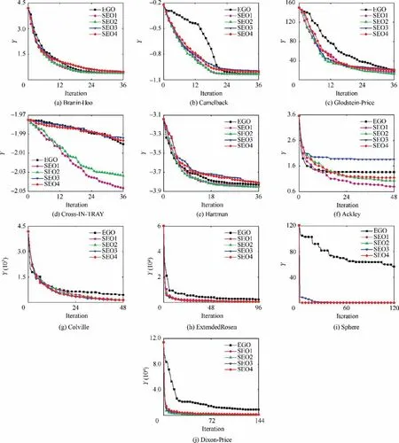
Fig. 6 Mean value of optimization results obtained by different ensemble models as a function of the number of cycles.

The considered optimization problem can be expressed as:

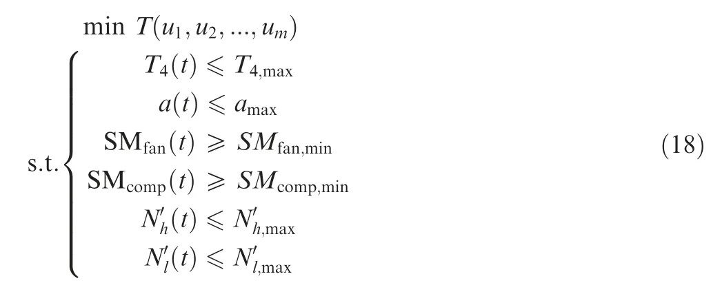
where Tdenotes the time consumption of engine acceleration,umdenotes the control variables of Bezier curves,and m is the number of control variables,and in the test,m was set as 20,t denotes the time,T4represents the high-pressure turbine inlet temperature,a denotes the excess air coefficient in the combustion chamber, SMfanand SMcompdenote the surge margin of fan and compressor, respectively, N’hand N’ldenote the speed variety ratio of high-pressure and low-pressure turbines, respectively.It should be noted that T is defined as the time consumption when the engine thrust(F)reaches a certain value.

3.3. Performance measure

The performance of the surrogate-based optimization algorithm is assessed using the final optimization result and convergence rate. As for the final optimization results, the Normalized Optimization Result (NOR) was defined as:

where yidenotes the optimization results obtained by the SBO algorithm after i optimization cycles, and yinidenotes the initial optimization value, and yoptdenotes the theoretical optimal value.

In order to measure the convergence rate, the Normalized Convergence Rate (NCR) was defined as:

where p denotes the maximum optimization cycles.

4. Results and discussion

4.1. Results comparison of different ensemble models

The mean value of the optimization results obtained by different ensemble models as a function of the number of cycles is presented in Fig. 6, where it can be seen that using the SEO accelerate the optimization process.

Table 4 Performance comparison of the EGO and SEO algorithms for the Branin-Hoo function.

Table 5 Performance comparison of the EGO and SEO algorithms for the Camelback function.

Table 6 Performance comparison of the EGO and SEO algorithms for the Glodstein-Price function.

Table 7 Performance comparison of the EGO and SEO algorithms for the Cross-IN-TRAY function.

The optimization results obtained by the EGO and SEO algorithms after each 6D optimization cycles are presented in Tables 4–13, where D denotes the number of dimensions of the test function, and the numbers in the brackets denote the NOR and NCR values. The best results in terms of NOR are marked in bold.

In almost all cases,the optimization results obtained by the SEO algorithm were better than those of the EGO algorithm after 6D optimization cycles in terms of both NOR and NCR. After 12D and 18D optimization cycles, the SEO algorithm based on the average ensemble model still performed better than the EGO algorithm for the Colville, ExtendedRosen, Sphere, and Dixon-Price test functions. However, for the other test functions,the performance of the SEO based on the average ensemble model was worse than that of the EGO algorithm. In addition, the SEO algorithm based on the pointwise ensemble model showed better performance than the EGO algorithm for all test functions.

The boxplots of the final optimization results are presented in Fig. 7, where it can be seen that the SEO algorithm performed better than the EGO algorithm in terms of both convergence and robustness for all high-dimension test functions. However, for the low-dimension test functions, theoptimization results obtained by the SEO algorithm based on the average ensemble model were worse than those of the EGO algorithm.The optimization results obtained by the SEO algorithm based on the pointwise ensemble model were better than EGO.

Table 8 Performance comparison of the EGO and SEO algorithms for the Hartman function.

Table 9 Performance comparison of the EGO and SEO algorithms for the Ackley function.

Table 10 Performance comparison of the EGO and SEO algorithms for the Colville function.

Table 11 Performance comparison of the EGO and SEO algorithms for the ExtendedRosen function.

Table 12 Performance comparison of the EGO and SEO algorithms for the Sphere function.

Table 13 Performance comparison of the EGO and SEO algorithms for the Dixon-Price function.

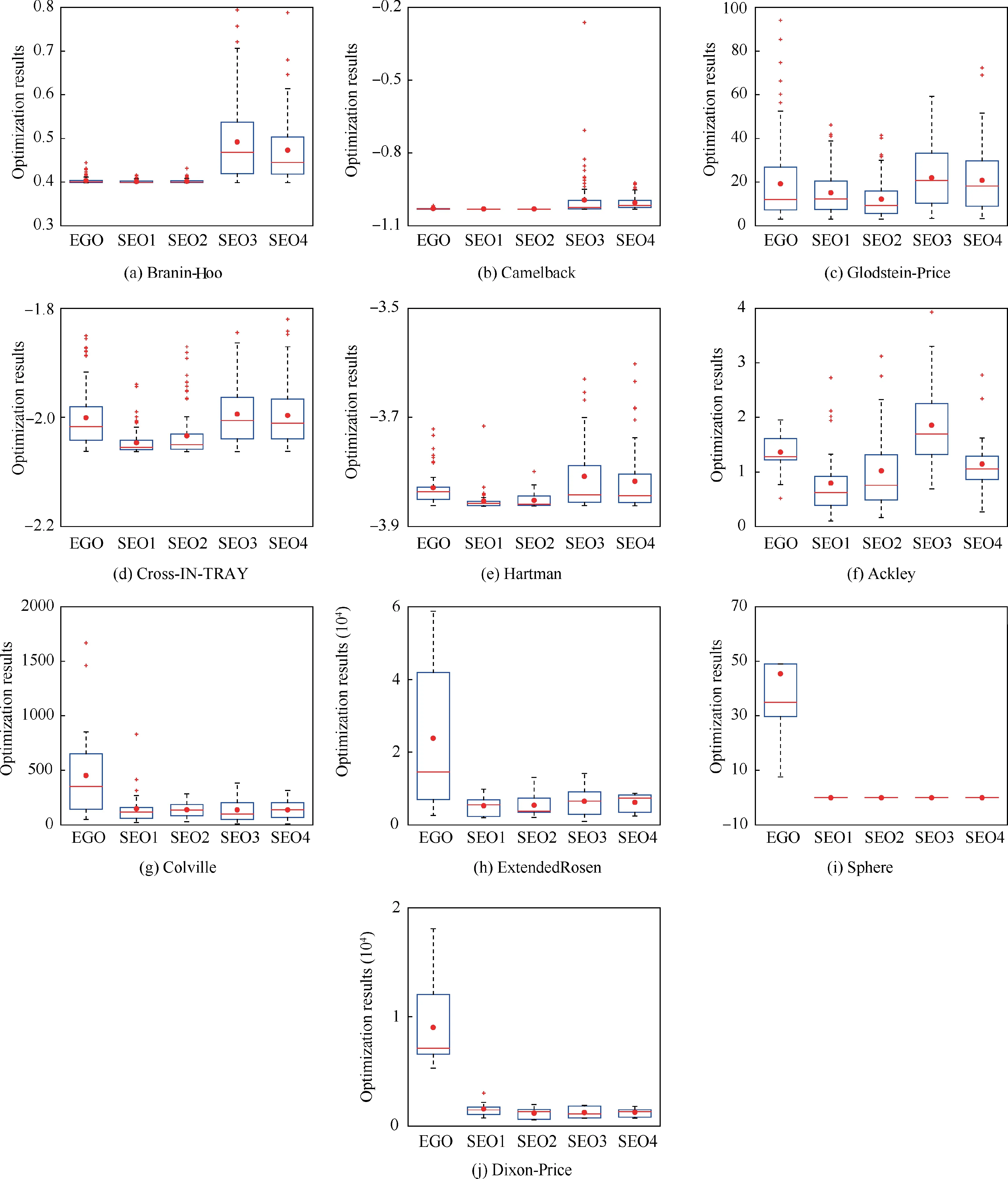
Fig. 7 Boxplots of the final optimization results obtained by different ensemble models.

The global accuracy of the initial ensemble model is usually better than that of the individual surrogate model. Therefore,in the beginning of the optimization process, the optimization results obtained by the SEO algorithm based on the ensemble model were better than those obtained by EGO algorithm.However,for some test functions,the final optimization results obtained by the EGO algorithm were better than those obtained by the SEO algorithm based on the average ensemble model.This was because,in the beginning,the performance of the optimization algorithm depended on the global accuracy of the surrogate model. However, the final optimization results depended on the local accuracy around the theoretically optimal solution. Compared to the average ensemble model, thepointwise ensemble model could adapt to the local characteristics of each individual surrogate model. As the number of observed points increased, the local accuracy around the optimal solution of the pointwise ensemble model was better than that of the average ensemble model in most cases. Thus, the pointwise ensemble model is more suitable for the SEO algorithm than the average ensemble model. However, for some test functions,the average ensemble model can provide similaraccuracy compared with the pointwise ensemble model.Therefore, the optimization results obtained by the SEO algorithm based on the average ensemble model were similar or even better than those obtained by the SEO algorithm based on the pointwise ensemble model, as presented for the Colville and Sphere test functions.

Table 14 Performance comparison of the SEO algorithm based on different surrogate models for the Branin-Hoo function.

Table 15 Performance comparison of the SEO algorithm based on different surrogate models for the Camelback function.

Table 16 Performance comparison of the SEO algorithm based on different surrogate models for the Glodstein-Price function.

Table 17 Performance comparison of the SEO algorithm based on different surrogate models for the Cross-IN-TRAY function.

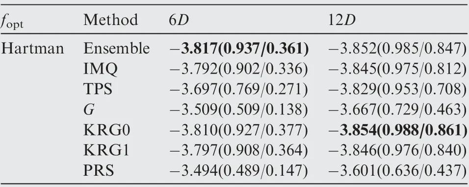
Table 18 Performance comparison of the SEO algorithm based on different surrogate models for the Hartman function.

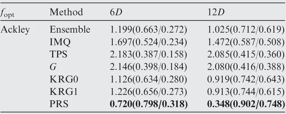
Table 19 Performance comparison of the SEO algorithm based on different surrogate models for the Ackley function.

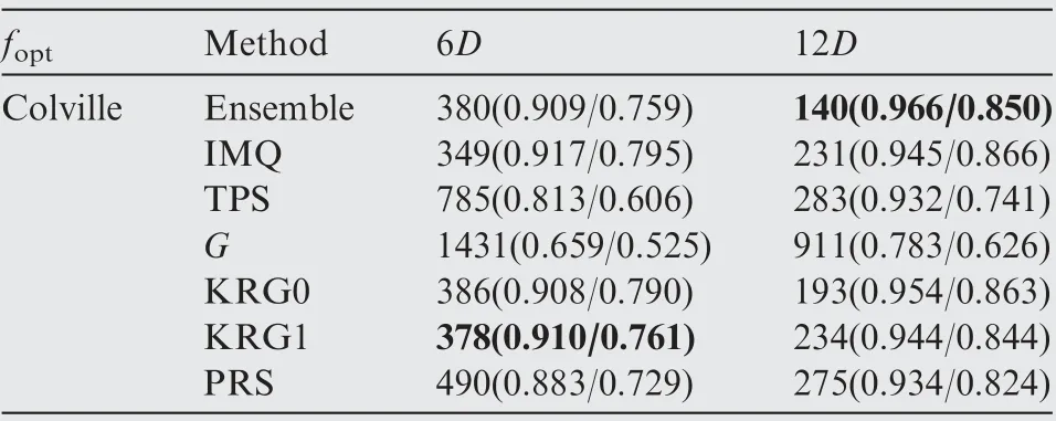
Table 20 Performance comparison of the SEO algorithm based on different surrogate models for the Colville function.

4.2. Results comparison of different surrogate models

The optimization results obtained by the ensemble model and different surrogate models after each 6D optimization cycles are presented in Tables 14-23, where the numbers in the bracket denote the NOR and NCR values,and the best results in terms of NOR are marked in bold. As shown in Tables 14-23, except for the Dixon-Price test function, the optimizationalgorithm based on the ensemble model performed better in terms of final optimization results and convergence rate than the optimization algorithm based on the individual surrogate model.

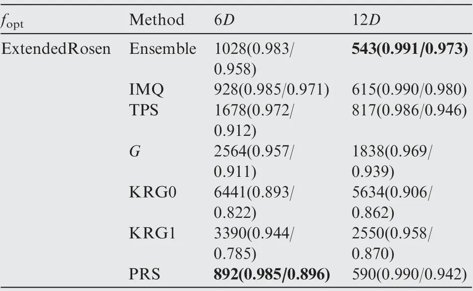
Table 21 Performance comparison of the SEO algorithm based on different surrogate models for the ExtendedRosen function.

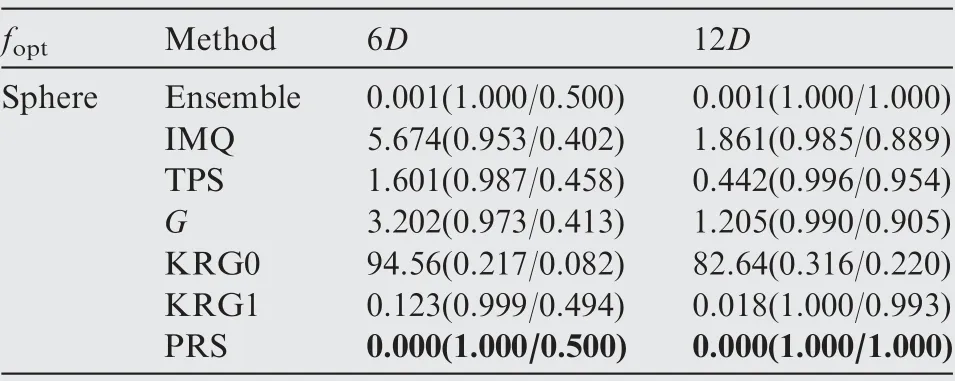
Table 22 Performance comparison of the SEO algorithm based on different surrogate models for the Sphere function.

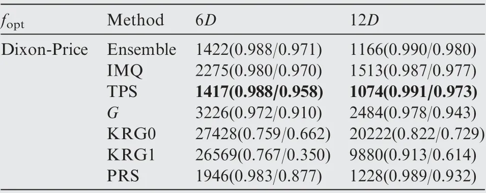
Table 23 Performance comparison of the SEO algorithm based on different surrogate models for the Dixon-Price function.

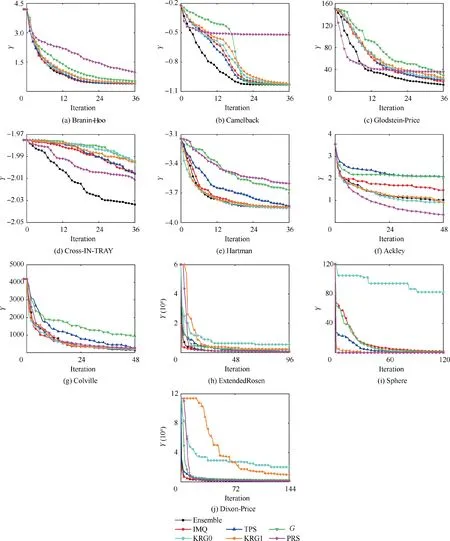
Fig.8 Mean value of optimization results obtained by ensemble model and different surrogate models as a function of number of cycles.

The mean value of the optimization results obtained by the ensemble model (SP2) and different surrogate models as a function of the number of cycles is presented in Fig. 8, where it can be seen that the optimization algorithm based on different surrogate model performed relatively different for different test functions. For instance, the optimization algorithm based on the PRS showed poor performance for the Branin-Hoo and Camelback test functions,but it showed good performance for the ExtendedRosen, Sphere, and Dixon-Price test functions.The optimization algorithms based on KRG0 and KRG1 showed good performance for the Branin-Hoo, Camelback,Glodstein, and Colville test functions, but they showed poor performance for the ExtendedRosen, Sphere, and DixionPrice test functions. In contrast, the optimization algorithm based on the ensemble model showed good performance for all test functions. Thus using the ensemble model improved the performance of the surrogate-based optimization algorithm.

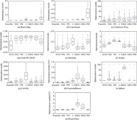
Fig. 9 Boxplots of the final optimization results obtained by ensemble model and different surrogate models.

The boxplots of the final optimization results are presented in Fig.9,where it can be seen that the optimization algorithm based on the ensemble model performed better than the optimization algorithm based on the individual surrogate model in terms of both convergence and robustness.The optimization algorithm based on the ensemble model did not achieve the best final optimization results for all test problems, but it provided the most stable optimization performance. The optimization algorithm based on the PRS outperformed the optimization algorithm based on the ensemble model for the Ackley test problem. However, the optimization algorithm based on the PRS showed poor performance for the Branin-Hoo and Camelback test problems. This was because the purpose of building the ensemble model was not to develop a more accurate surrogate model than the individual surrogate model for a certain problem,but to provide a stable prediction performance for various problems. Therefore, although the accuracy of the ensemble model was worse than that of the most accurate individual surrogate model in some cases, the optimization results obtained by the ensemble model were generally better than the best optimization results obtained by the individual surrogate model.

4.3. Results comparison of different surrogate models and uncertainty estimators

The comparison of the NOR and NCR values of the optimization algorithms based on the ensemble model(SP2)and different individual surrogate models with different uncertainty estimators is given in Table 24,where the NOR value is shown in the first row in each cell,and the NCR value is shown in the second row in each cell. The best results in terms of NOR are marked in bold in each cell.

The optimization results obtained by the ensemble model with the GUE were mostly better than those obtained by the other algorithms. In the optimization algorithm based on the ensemble model, the GUE outperformed KUE. However, in the optimization algorithm based on the individual surrogate model, there was no significant advantage of utilizing the GUE. The main advantage of using the GUE over the KUE is that it can provide an uncertainty estimator for any surrogate model. Thus, the GUE is more suitable to provide an uncertainty estimator for the ensemble model than the KUE.

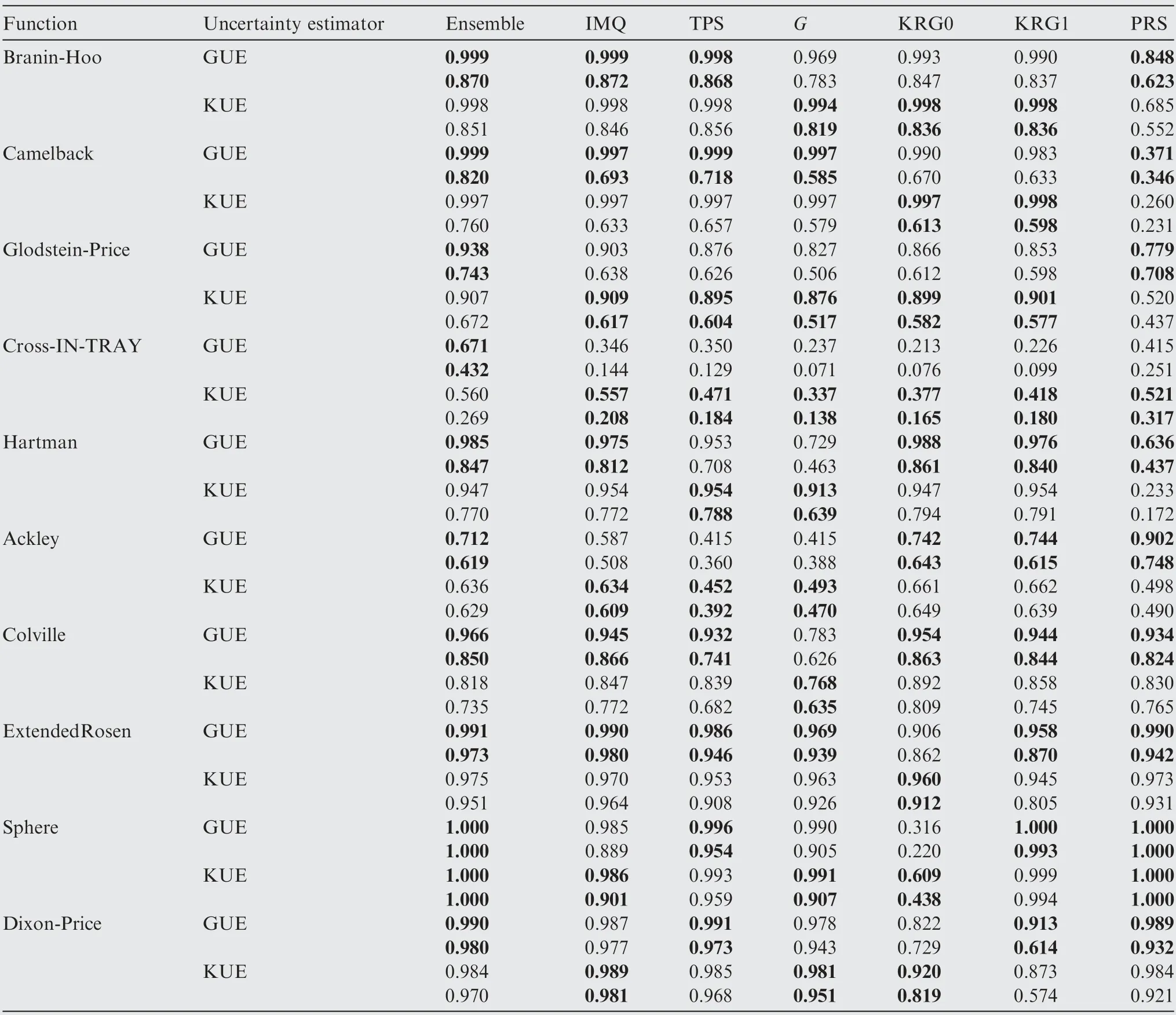
Table 24 Performance comparison of the SEO algorithm based on different surrogate models and uncertainty estimators.

4.4.Global optimization control of turbo-fan engine acceleration schedule design

The optimization results obtained by the SEO and EGO algorithms are presented in Fig.10,where can be seen that the optimized control schedule obtained by the SEO algorithm was better than that obtained by the EGO algorithm in terms of the time consumption of engine acceleration.

The comparison of the NOR and NCR values of the optimization algorithms based on the ensemble model (SP2) and different individual surrogate models with different uncertainty estimators is presented in Table 25, where the NOR value is shown in the first row in each cell and the NCR value is shown in the second row in each cell. The best results in terms of NOR are marked in bold in each cell. It should be noted that yoptin Eq. (18) was set as the optimization result obtained by the ensemble model and GUE for this problem.As shown in Table 25, the optimization results obtained by the ensemble model with the GUE were better than those obtained by the other algorithms. In the optimization algorithm based on the ensemble model, the GUE outperformed the KUE.

5. Conclusions

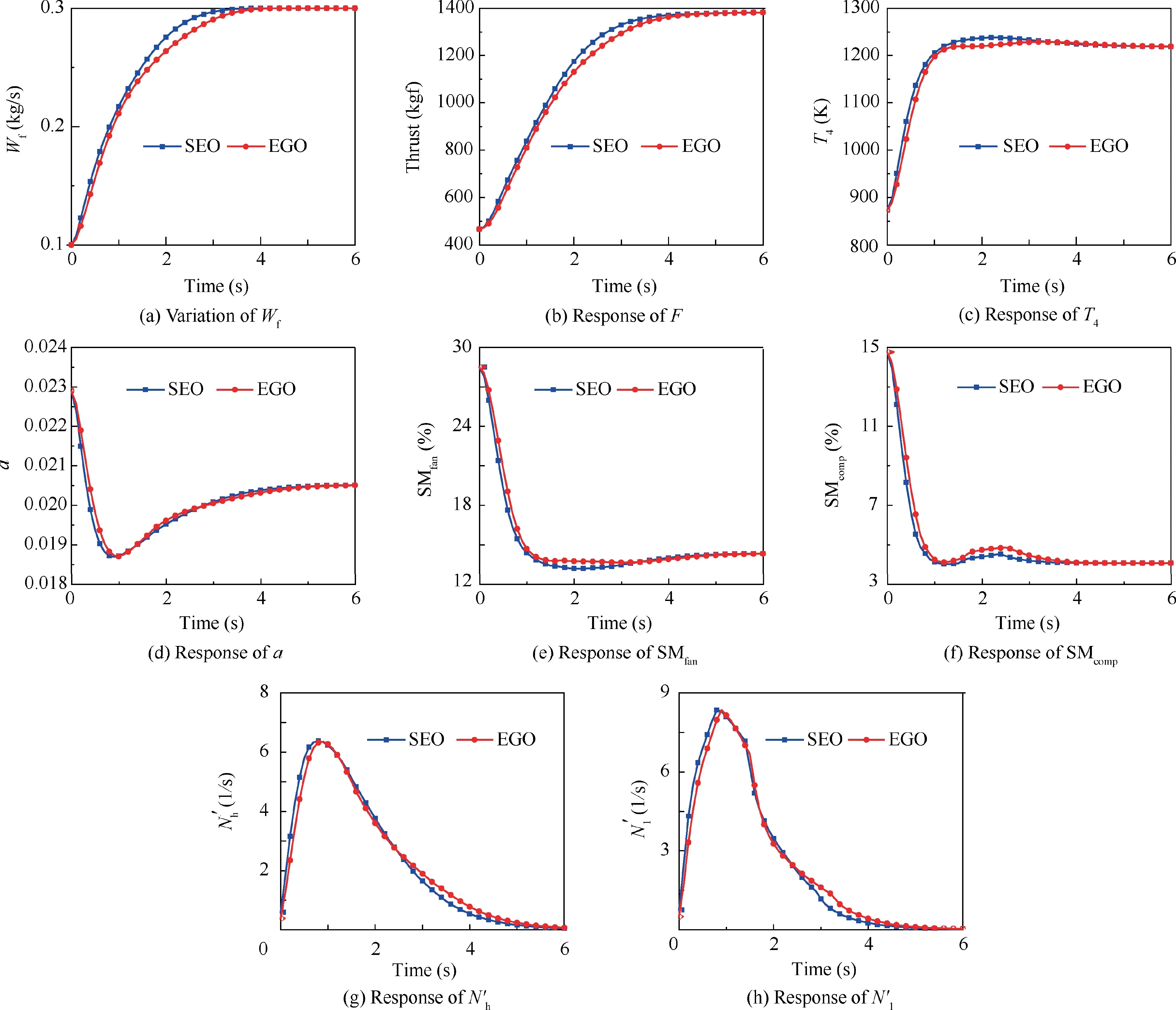
Fig. 10 Optimization results obtained by SEO and EGO algorithms.

Table 25 Performance comparison of the SEO algorithm based on different surrogate models and uncertainty estimators.

In this paper,a SEO algorithm is developed using the GUE.In order to verify the performance of the proposed algorithm,the algorithm is validated and assessed by ten well-known benchmark problems.The developed algorithm is applied to the global optimization control of turbo-fan engine acceleration schedule design. The results show that using the SEO algorithm can accelerate the optimization process. However, for some of the used test functions, the SEO algorithm based on the average ensemble model does not perform better than the EGO algorithm in terms of the final optimization results.However, the SEO based on the pointwise ensemble model outperforms the EGO algorithm in terms of both the final optimization results and the convergence rate. Besides, the optimization results obtained by the pointwise ensemble model are mostly better than the best optimization results obtained by the individual surrogate model. In the optimization algorithm based on the ensemble model, the GUE outperforms the KUE,but in the optimization algorithm based on the individual surrogate model, there is no significant advantage of utilizing the GUE.In future research,the individual surrogate models and their weight factors of the ensemble model could be used to generate a new sample point, which is expected to accelerate the optimization process.

Declaration of Competing Interest

The authors declare that they have no known competing financial interests or personal relationships that could have appeared to influence the work reported in this paper.

Acknowledgements

The authors would like to express their gratitude for the financial support of the National Natural Science Foundation of China (Nos.52076180, 51876176 and 51906204)and National Science and Technology Major Project, China (No. 2017-I-0001-0001).