Influence of leading edge with real manufacturing error on aerodynamic performance of high subsonic compressor cascades

Chi MA,Limin GAO,*,Haohao WANG,Ruiyu LI,Baohai WU

a School of Power and Energy,Northwestern Polytechnical University,Xi’an 710129,China

b The National Key Laboratory of Aerodynamic Design and Research,Xi’an 710129,China

c Key Laboratory of Contemporary Design and Integrated Manufacturing Technology of Ministry of Education,Northwestern Polytechnical University,Xi’an 710072,China

KEYWORDS

Abstract To investigate the influence of real leading-edge manufacturing error on aerodynamic performance of high subsonic compressor blades,a family of leading-edge manufacturing error data were obtained from measured compressor cascades.Considering the limited samples,the leadingedge angle and leading-edge radius distribution forms were evaluated by Shapiro-Wilk test and quantile-quantile plot.Their statistical characteristics provided can be introduced to later related researches.The parameterization design method B-spline and Bezier are adopted to create geometry models with manufacturing error based on leading-edge angle and leading-edge radius.The influence of real manufacturing error is quantified and analyzed by self-developed non-intrusive polynomial chaos and Sobol’indices.The mechanism of leading-edge manufacturing error on aerodynamic performance is discussed.The results show that the total pressure loss coefficient is sensitive to the leading-edge manufacturing error compared with the static pressure ratio,especially at high incidence.Specifically,manufacturing error of the leading edge will influence the local flow acceleration and subsequently cause fluctuation of the downstream flow.The aerodynamic performance is sensitive to the manufacturing error of leading-edge radius at the design and negative incidences,while it is sensitive to the manufacturing error of leading-edge angle under the operation conditions with high incidences.

1.Introduction

Highly loaded compressors raise an urgent need for the improvement of the thrust to weight ratio of aircraft engines.1Highly loaded working condition is accompanied by the increase of inflow Mach number,even higher than the sound speed at rotor tip.The leading edge of highly loaded compressor blades is typically with small radius to suit the severe inflow environment.This geometrical feature results in large curvature and it is difficult for computer numerical control(CNC)machine tools to manufacture.2Manufacturing error is inevitable during the complex manufacturing process even with high precision.The measurement data of leading-edge manufacturing error exhibits random deviations from their design shape and size,3which belongs to aleatory uncertainty.However,the aerodynamic performance(efficiency and pressure ratio)of the compressor is extremely sensitive to the leading edge which has an impressive effect on shock structures,boundary layer developing and blade profile loss.4-6Moreover,the continuous curvature leading edge can decrease the formation of separation bubble;7,8larger leading-edge wedge angle can weaken the laminar separation in low Reynolds number;9compared with circle radius,ellipse shape can change the pressure distribution and acceleration process at leading edge in high turbulence level.10The spike height which changes with leading edge affects the unsteady transition process.11Therefore,it is valuable to study the influence of the leading edge with the real manufacturing error for understanding the real compressor performance.

In 1994,Lykins et al.12suggested that the problems in manufacturing processes need concern for the requirement of highperformance engine.Lejon et al.13found that the geometric scatter impacts the pressure distribution along the leading edge and shock position using numerical simulation.Lange et al.14proved that leading-edge thickness manufacturing error is the most important on the aerodynamic performance.An experimental investigation on leading-edge manufacturing error showed that the leading-edge radius manufacturing error has a great influence on aerodynamic performance of compressor blade under high subsonic inflow condition.15Cheng et al.16proved that leading-edge angle affects the efficiency using an orthogonal experiment method to study six manufacturing errors.Thus,leading-edge radius and angle are two critical parameters both in design and manufacturing detection of compressor blades.

With respect to the construction of leading edge with manufacturing error,it is common to base on scanned geometrical coordinates around leading edge.13,17However,Nigro et al.18realized the profile by defining a covariance between the surface points.Goodhand17used self-designed method to alter the radius of curvature,and the variations of leading edge from lots of measured blade data were imposed back onto the same blade.Dow19and Yan et al.20imposed the manufacturing error on a design blade by Karhunem-Loeve expansion for a non-stationary Gaussian process,respectively.Cai et al.15constructed the leading edge with manufacturing error by changing the leading-edge radius.Using scanned geometrical coordinates to construct the leading edge is likely to contain characteristics which are not quite critical to the aerodynamic performance.But changing leading-edge radius alone just can describe part influence of leading-edge manufacturing error.In this paper,leading-edge angle along with leading-edge radius as two key parameters to the aerodynamic performance are employed to construct the leading edge.

The leading-edge manufacturing error variation range is various to different components,13,17,21and it also provides the geometrical bounds of the leading-edge construction.Furthermore,the statistical characteristics of manufacturing error affect the evaluated influence on aerodynamic performance.3,22,23Thus,the setup based on practical engineering is beneficial to obtaining meaningful results.For high subsonic compressor blades,the stochastic characteristics of real leading-edge manufacturing error data still need analysis in detail.Anderson-Darling test,14frequency histogram24and Kolmogorov-Sminov test25are used to get the distributions of manufacturing error of compressor parameters,and the successful works of these methods are based on a rich set of data.However,limited real measurement data is a common facing problem due to high measurement cost or time-consuming experiments.A proper way to deal with limited measurement data is essential for industrial problems.

In the current paper,the influence of leading-edge manufacturing error on aerodynamic performance of high subsonic compressor cascades is analyzed based on real measurement data.Two statistical methods are introduced to evaluate the distribution form and stochastic characteristics.The leading edge is reconstructed using Bezier and B-spline based on leading-edge radius and leading-edge angle.The key factor for triggering the uncertainty of the flow field is discussed in detail by flow field analysis.

2.Hypothesis testing methodologies and statistical characteristics of leading-edge manufacturing error based on limited measurement data

2.1.Hypothesis testing methodologies

Shapiro-Wilk test(S-W test)and quantile-quantile plot(Q-Q plot)are two kinds of hypothesis testing methodologies.Neither of them can get the sufficiently definite test result of estimated distribution alone facing small sample space size problem.To deal with it,S-W test and Q-Q plot are introduced to assess the distribution form and statistical characteristics.The consistent distribution form estimated from the two methods is a reliable way to deal with the limited measurement data fitting Gaussian distributions.

2.1.1.Shapiro-Wilk test

S-W test divides the square of a linear combination of the sample order statistics by the symmetric estimate of variance.It is powerful to testify the probability distribution for sample space less than 50.26The test result is evaluated by W and its value lies in the range from 0 to 1.If W is smaller than the set threshold value,then the samples do not satisfy the hypothesis.For an order random samples z1＜z2＜...＜zmfrom a continuous population z of m,W is defined by

2.1.2.Quantile-quantile plot

Traditionally,the Q-Q plot27is a graphical technique for determining whether two data sets come from populations with the same distribution based on the cumulative distribution functions.It is an appealing method owing to the easily intuitive linearity.

Assume that F(xi)is the cumulative distribution function,and the quantile q(zi)is the inverse function of F(zi),which is presented as F-1.For estimating the Gaussian distribution z～N(μ,σ2)with the mean valueμand standard deviation σ,q(zi)can be calculated by

The scatter plot on the coordinate plane using(qi,xi)is the Gaussian distribution of Q-Q plot.If the scatter plot is from Gaussian distribution,Q-Q plot will be a straight line.The slope of the line is the standard deviationσand intercept is the mean valueμ.

2.2.Statistical characteristics of leading-edge manufacturing error

As shown in Fig.1,the real leading-edge manufacturing error is decoupled into two parameters:leading-edge angle(χ1)and leading-edge radius(R).The leading-edge angle(χ1)is the angle between chord and tangent of the initiation point of camber line.It is a vital parameter related to incidence.The leading-edge radius(R)defines the radius of the first incircle at the leading part of the blade.It affects the flow pattern and flow separation.χ1and R are extracted from measurement geometric coordinate data from the manufactured blades.The difference ofχ1and R between manufactured and design blade is the manufacturing error.The evaluation results of limited 28 measurement data of high subsonic compressor blades from coordinate measuring machine28by S-W test and Q-Q plot both show thatχ1and R satisfy Gaussian distribution as shown in Figs.2 and 3.Specifically,χ1-design=45.830 °,σ(χ1)=0.720 °,σ(χ1)/χ1-design=1.57%;Rdesign=0.521 mm,σ(R)=0.042 mm,σ(R)/Rdesign=8.06%.

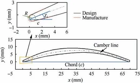
Fig.1 Compressor blade.

3.Uncertainty quantification methodology and research scheme

3.1.Non-intrusive polynomial chaos expansion

The self-developed non-intrusive polynomial chaos(NIPC)expansion that has been validated in previous paper29,30is used to quantify the influence of leading-edge manufacturing error.This method uses a series stochastic orthogonal polynomial Ψjx()with deterministic coefficients ajto express a stochastic output Y.NIPC is more attractive than other uncertainty quantification methods owing to its high efficiency and accuracy.

If Y is the stochastic output of the n-dimensional random independent variable vector x=［x1，...，xi，...，xn］,it can be written as

where Q is the number of polynomials,and ajis the coefficient of each polynomial.Ψjx()is the jth multivariate orthogonal polynomial,and it can be computed using the product of univariate orthogonal polynomialψj()x():

In the current paper,x consists of leading-edge angle(χ1)and leading-edge radius(R).The stochastic output Y can be total pressure loss coefficient(ϖ),and the static pressure ratio(π).Hermite polynomial is used asψj()x()since the uncertaintiesχ1and R have proofed to fit Gaussian distribution.According to the previous work31and papers,32,33the fourth-order(p=4)NIPC is chosen to quantify the influence of uncertain leading-edge parameters(n=2)on aerodynamic performance.The term number Q=15 in Eq.(4)can be calculated using Eq.(6):

According to p=4 and n=2,25=p+1()ncollocation points based on full tensor-products Gaussian quadrature are chosen for uncertainty quantification under each operating condition.

The mean valueμ(Y)and the varianceσ2(Y)of a stochastic output Y are calculated as

Deterministic coefficients ajin Eq.(4)are computed using Galerkin projection34:

where＜·,·>denotes the inner product,and w x()is the weight over the supportΩ.

Fig.2 Q-Q plots of manufacturing error ofχ1 and R.

Fig.3 Frequency histogram and probability density function of manufacturing error ofχ1 and R.

3.2.Sobol’indices based on non-intrusive polynomial chaos expansion

The Sobol’indices SU based on non-intrusive polynomial chaos(NIPC)are developed to evaluate the contribution of the random variable xito the stochastic output Y.Sobol’indices can quantify the contribution of variables by decomposingσ2(Y)into individual contributions of input variables xiand interaction contributions between different input variables.The input variables leading-edge angle(χ1)and leading-edge radius(R)are written as xχ1and xR,respectively.Sobol’indices SUχ1,SURand SUR&χ1are defined as

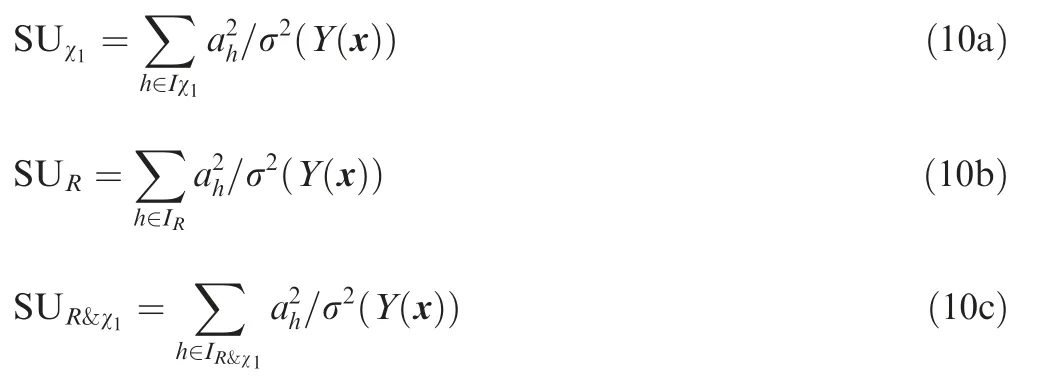
where Iχ1corresponds to the polynomials only depending on xχ1;in the same way,IRcorresponds to the polynomials only depending on xR.With respect to the interaction contribution between xχ1and xR,IR&χ1corresponds to the polynomials depending on both xχ1and xR.

Sobol’indices are satisfied with

The first-order indices SUχ1and SURweight the influence of individual alone while the higher-order index SUR&χ1represents the coupled influence of two parameters.

4.Research object and operating condition setting

As shown in Fig.4,the geometrical model is a twodimensional high subsonic compressor cascade.Its chord length(c)is 69.95 mm,solidity(τ=c/t)is 2.3 and stagger angle(β)is 26.58 °.Upstream and downstream extension distance are one chord and 2.5 chords,respectively.

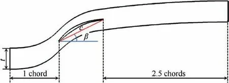
Fig.4 Computational domain.

The cascade described by camber line and thickness distributions is shown in Fig.5.Camber line is parametric design by Bezier curve with 13 control points.The profile of cascade parametric is designed by B-spline and imposed with modifiable radius leading edge.The thickness distribution of cascade is controlled by 15 pair thickness values along the chord.The leading-edge angle is changed by altering the location of the Bezier control point 2.The leading-edge variation range is the first 10% of the chord.

Fig.6 illustrates that all the leading edge imposed leadingedge manufacturing error corresponding to the collocation points of NIPC in Section 3.1.The dashed curve represents the design leading edge.Inflow Mach number Ma1=0.7 with various incidences(i)are selected as the operating conditions based on previous experimental research,15since that research has proved that the effect of manufacturing error is significant at Ma1=0.7.

The steady 3D compressible RANS equations are solved with finite volume method based on the Spalart-Allmaras turbulence model.The second-order central difference scheme is chosen for the spatial discretization of the equations.The time discretization is done using the explicit four-step Runge-Kutta scheme.The mesh of the cascade passage was generated with O4H topology.The minimum grid spacing of 1×10-6m was applied on the solid walls to make the non-dimensional wall distance y+no more than 8 at the walls.Total pressure,total temperature and inlet flow angles were given uniformly at the inlet boundary.Mass flow rate boundary condition was designated at the outlet plane to ensure the required uncertain inflow conditions.

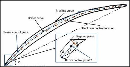
Fig.5 Cascade parametric design.

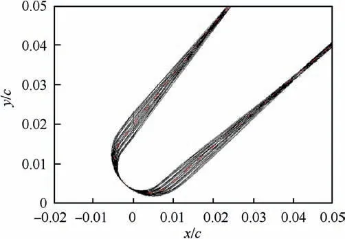
Fig.6 Leading edges used in NIPC.

5.Results and discussion

5.1.Influence of uncertain leading-edge manufacturing error on performance

The mean valueμsuperimposed with standard deviationσof the static pressure ratioπand the total pressure loss coefficients ϖat various incidences(i)are shown in Fig.7.Design values without uncertainty disturbance are added in the figure as reference to compare the difference between the values with and without uncertainty.The grey region represents the fluctuation range ofπandϖ,the boundary of grey region is determined by mean value ofπandϖplus and minus one time’s standard deviation.μ(π)goes up with the increase of i and then decreases at i=7 °.μ(ϖ)goes down as i changes from 0 ° to design incidence 2.5°,and then rises as i increases.Under design operating condition,the mean valueμ(π)andμ(ϖ)are identical to the design values.In off-design i,most of the operating conditions are also identical to the design values.However,there is an error that can be observed in some operating conditions ofϖ.The effects of uncertainties can be negative or positive under difference conditions.Compared withπ,ϖis more sensitive to the disturbance of uncertain geometry.

Fig.8 shows thatσ(π)andσ(ϖ)vary with i.The variation trend of them are similar.As i increases,they both drop first at i=2.5°and then rise.The biggestσ(π)andσ(ϖ)both occur at i=7 ° and the smallest values both occur at design incidence i=2.5 °.The absolute value of them are similar,but the biggest percentage to the corresponding mean valuesσ(π)μ(π)andσ(ϖ)/μ(ϖ)are 0.49% and 11.38% occurring at i=7 °,respectively.These phenomena also confirm thatϖis more sensitive.

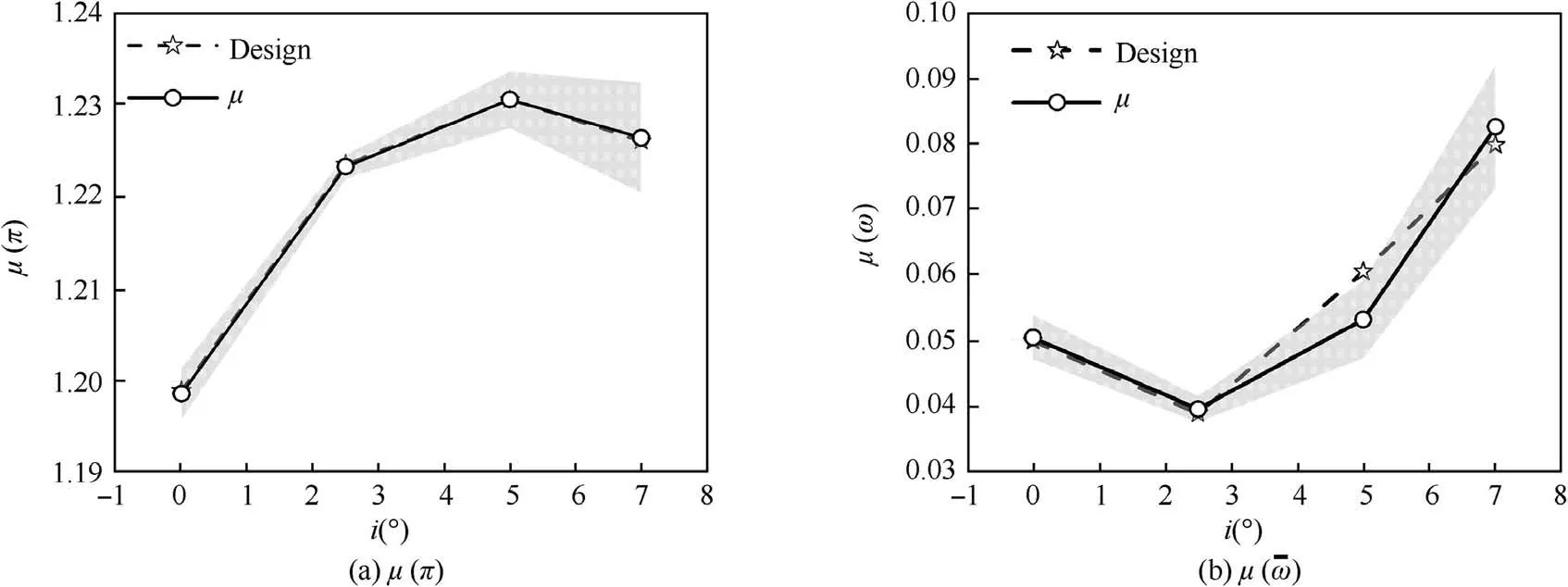
Fig.7 Aerodynamic performance under uncertain leading-edge manufacturing error.

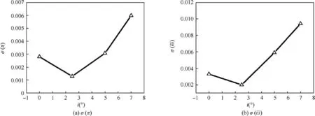
Fig.8 Standard deviation of aerodynamic performance under uncertain leading-edge manufacturing error.

Fig.8 just provides the fluctuation amplitude,but the information about the specific probability distribution is missing.The probability density functions(PDF)ofπandϖare illustrated in Fig.9 by performing 5000 Monte Carlo Simulations for each operating condition.The distribution forms are different,some are very similar to the typical distributions like the PDF ofπat i=0°,but most of PDFs show an arbitrary form.It can be concluded that the distribution form of output is not closely related to the PDF of input uncertainties.The PDFs in

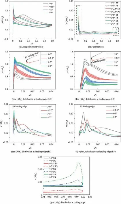
Fig.10μ(Mais)andσ(Mais)distribution along chord at various i.

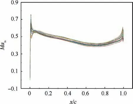
Fig.11 Mais distribution on PS at i=7 °.

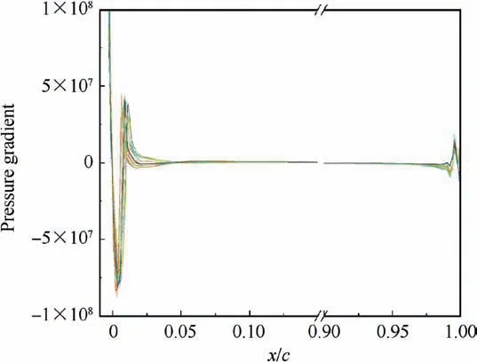
Fig.12 Pressure gradient along chord on PS at i=7 °.

5.2.Influence on flow field and mechanism analysis

Fig.10 shows isentropic Mach number(Mais)distribution along the chord and enlarged figures at leading edge and trailing edge.Fig.10(a)shows that,as i increases,the peakμ(Mais)moves forward but the peak value goes down.The reason for this tendency is that the incidence variation changes the passage from a converging-diverging passage to a converging one,which alters the transformation of kinetic energy and pressure energy.

The influence of uncertain leading-edge manufacturing error on Maisconcentrates at the leading edge and trailing edge as shown in the dashed line box of Fig.10(b).Fig.10(c)-10(d)illustrate the zoomed-in picture at the leading edge on the suction surface(SS)and pressure surface(PS)superimposed with standard deviation.In Fig.10(c),the leading peak μ(Mais)represents the‘‘spike”on the SS.As i increases,the location of the spike moves forward,and i=7 ° is the most affected operating condition.But the trend on the PS is opposite as shown in Fig.10(d),i=0°is the most affected,and the maximum peakμ(Mais)occurs at i=0 °.

When taking a close look at the fluctuation amplitude as shown in Fig.10(e)-10(f),the biggest fluctuation amplitude happened at i=7 °in the location of the spike on the SS.Although the fluctuation amplitude distributions in Fig.10(e)-10(f)manifest that i=2.5 ° keeps a big fluctuation amplitude in a wider region along the chord at the leading edge,it shrinks rapidly to the smallest as shown in Fig.10(a)(the red belt is the narrowest).i=7 ° does not show a big fluctuation amplitude in the initial region of the leading edge except the spike on the SS,but it remains a certain fluctuation amplitude in the whole chord and even grows higher at the trailing edge as shown in Fig.10(g).By contrast,i=0 ° presents a high fluctuation amplitude at leading edge on the PS(Fig.10(f))but the relative uniform static pressure distribution near the PS guides the flow back to uniform and performs a small fluctuation amplitude at the trailing edge of the cascade(Fig.10(b)).

According to the above discussion,i=7 ° is the most sensitive.Fig.11 demonstrates the Maisdistribution on the PS at i=7°at all the collocation points.It can be observed that all the curves have the same tendency excepted the first 10% of the chord disturbed by uncertain leading-edge manufacturing error but Maisshows a big dispersibility from x/c≈10% of the chord.In Fig.12,the pressure gradient representing the change of Maisjust fluctuates in the leading and trailing edge.The uniformity of the pressure gradient in the range of x/c=0.05 to x/c=0.95 proves that the sudden increase ofσ(Mais)at trailing edge in Fig.10(g)cannot be triggered by the pressure gradient on the PS in such a subsonic flow field.

In Fig.13,flow fields of five collocation points having various topologies are chosen(named sample 1 to sample 5)to describe the flow structure variation at the trailing edge at i=7 °.The number variation of nodes(N),saddle points(S)and half nodes(N′)change with the flow structure in the back part of the blade.Note that the location and scope of trailing-edge shedding vortex(TSV,N2)are directly affected by the separation vortex(SV,N1)on the SS.The scope of SV itself is also variable.The interaction between TSV(N2)and SV(N1)results in different topologies and generates saddle points(S1,S2and S3),more nodes(N3,N4)and half nodes(nodes on the wall,N′1).In other words,SV(N1)alters the shape and scope of TSV(N2)and finally changes Maisnear the trailing edge on PS as mentioned in Fig.10(g).The location and scope of TSV(N2)are tremendously different in the flow field of each collocation point,which results in pressure fluctuation on the PS.Therefore,the topology change is fundamental to the highσ(Mais)in this region.

Fig.14 presents geometry models at collocation points with maximum positive/negative leading-edge radius and angle manufacturing error along with the design leading edge.The maximum positive/negative leading-edge radius manufacturing error R are marked with R+and R-.Similarly,the maximum positive/negative leading-edge angle manufacturing errorχ1are marked with A+and A-.These five samples are discussed in detail to investigate the influence of uncertain leading-edge manufacturing error on the flow field.

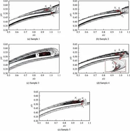
Fig.13 Streamline on SS and trailing edge.

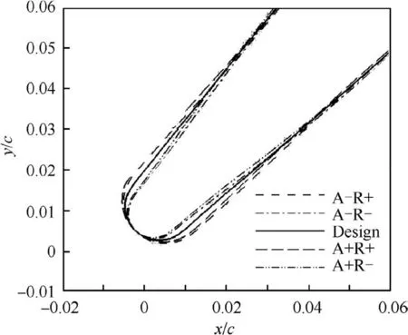
Fig.14 Leading edge of five collocation points.

Fig.15 shows the streamlines and normalized static pressure distributions.It can be observed that the uncertain leading edge R andχ1apparently alter the streamwise scope of the separation bubble on the SS at i=7.R controls the acceleration process from the stagnation point and static pressure distribution around the leading edge whileχ1alters the effective incidence.The pressure gradient on the SS and highspeed local flow behind the leading-edge acceleration process trigger the separation bubble.By comparing the five cases in Fig.15,bigger R always brings large-size separation bubbles.The separation bubble,static pressure distribution on the SS together with high-speed flow intensify the influence of the leading edge originated from the stagnation point.Fig.16 shows that the location of stagnation point is moving to the PS as the incidence increases,but small variation range in different incidences are almost the same.It can be concluded that the location of the stagnation point on the leading edge does not change too much.The uncertain R andχ1alter the flow acceleration from the stagnation point,make the fluctuation of the spike,and then intensively disturb the downstream flow field at the trailing edge.

Fig.17 displays the Vxdistribution,whereΔx/c is normalized chord length.Negative Vxrange represents the streamwise scope(Δx/c)of the separation bubble at collocation points.Among three positive incidence operating conditions,i=7 °has the maximumΔx/c.Δx/c of i=0° is bigger than that of i=7 °,but the separation of i=0 °occurs on the PS and the moderate pressure gradient suppresses the effect caused by separation bubble.Comparing the Vxreattached on the profile at three positive incidences,Vxdecreases as incidence increases.The decreased kinetic energy weakens the ability of the flow to withstand the adverse pressure gradient and this situation is prone to induce the boundary layer separation on the SS.

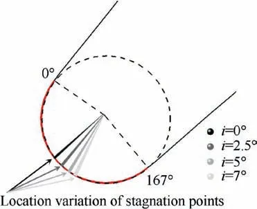
Fig.16 Location variation of stagnation points at four incidences.

Fig.18 shows theσ(ϖ)distribution,which can describe how the influence of uncertain leading-edge manufacturing error propagates in the flow field.The local high value means large fluctuation amplitude ofϖ.At design incidence i=2.5°,σ(ϖ)keeps low for the whole flow field,and there is only a small amplitude fluctuation in the region of the separation vortex.At i=0°,the highσ(ϖ)gathers on the front part of the PS at i=0°.In contrast,local high value occurs at the leading edge on the SS at i=5°and i=7°.The local high value near the SS caused by the uncertain leading-edge manufacturing error are similar at i=5 ° and i=7 °.The highestσ(ϖ)occurring at the downstream of the passage is associated to the trailing-edge shedding vortex,which is a quintessential flow structure in an unsteady flow field.Compared with i=2.5 °,the variation ofσ(ϖ)intensifies at i=5 ° and i=7 °.Note that at i=7 °,a local highσ(ϖ)region can be observed at the trailing edge on the PS.The trailing edge interacting with trailing-edge shedding vortex and separation vortex jointly results in the behavior of regular high-value spot downstream.

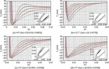
Fig.17 Vx along chord.

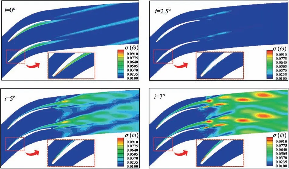
Fig.18σ(ϖ)distribution at various i.

Fig.19 displays the Sobol’s indices of uncertain R andχ1to σ2(ϖ)at various i.At i=0°and i=2.5°,ϖis sensitive to R while the influence ofχ1is marginal.As i increases to 5°,the importance ofχ1goes up.At i=7 °,χ1becomes the most influential parameter with SUχ1=61%.According to the data displayed in Section 2.2,σ(χ1)/χ1-design=1.57%whileσ(R)/Rdesign=8.06%.The fluctuation percent ofχ1is much smaller than R,which also stresses the importance ofχ1at high incidences.This outcome implies that leading edge should be paid great attention whether in detecting machining error or tolerance design of compressor besides the leading-edge radius.

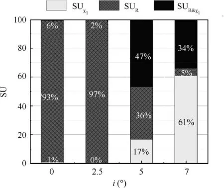
Fig.19 Sobol’s indices of R andχ1 toσ2(ϖ).

6.Conclusions

In this study,the influence of real leading-edge manufacturing error on aerodynamic performance of a high subsonic compressor cascade is investigated using self-developed NIPC and Sobol’indices.Hypothesis testing methods,S-W test and Q-Q plot,are introduced to assess the probability distribution forms of R andχ1.According to the statistical analysis of measuring experimental data and uncertainty quantification results,the primary conclusions can be summarized as follows:

(1)The S-W test and Q-Q plot work well to deal with the limited measurement data fitting Gaussian distribution like R andχ1.The fluctuation amplitude of R andχ1areσ(χ1)=0.720 °(σ(χ1)/χ1-design=1.57%)andσ(R)=0.042 mm(σ(R)/Rdesign=8.06%).The statistical characteristic values of manufacturing error from the real measurement data can be introduced to other related researches that focus on manufacturing error and tolerance design in similar cascades.

(2)Compared withπ,ϖis more sensitive to the uncertain leading-edge manufacturing error.The high ratioσ(ϖ)/μ(ϖ)=11.38% at i=7 ° stresses the importance of uncertainty quantification in the assessment of the aerodynamic performance caused by uncertain leading-edge manufacturing error,especially under off-design operating conditions.

(3)The influence of uncertain leading-edge manufacturing error on flow field shows that the high fluctuation amplitudeσ(ϖ)downstream of the passage is originated from the flow acceleration in the leading edge.High fluctuated spike and reduced kinetic energy under high positive incidence operating conditions intensify the separation vortex on the SS,and this separation vortex interacting with trailing-edge shedding vortex induces the various flow structures near the trailing edge.

(4)The most sensitive factor affectingσ2(ϖ)changes with the operating conditions.When the compressor cascade works at the design or negative incidences,the uncertainty of R should be checked carefully in the process of detecting machining error.The influence ofχ1should be paid great attention when the compressor cascade works at high incidences since it contributes to over 60%ofσ2(ϖ)according to the sensitive analysis results.

Declaration of Competing Interest

The authors declare that they have no known competing financial interests or personal relationships that could have appeared to influence the work reported in this paper.

Acknowledgements

This study was co-supported by the National Natural Science Foundation of China(No.51790512),the 111 Project(No.B17037),the National Key Laboratory Foundation,Industry-Academia-Research Collaboration Project of Aero Engine Corporation of China(No.HFZL2018CXY011-1)and MIIT.