Framework and development of data-driven physics based model with application in dimensional accuracy prediction in pocket milling

Zhanying CHEN,Liping WANG,Jiabo ZHANG,Guoqiang GUO,Shuailei FU,Chao WANG,Xuekun LI,*

a Department of Mechanical Engineering,Tsinghua University,Beijing 100084,China

b State Key Lab of Tribology,Tsinghua University,Beijing 100084,China

c Beijing Spacecrafts,China Academy of Space Technology,Beijing 100094,China

d Shanghai Spaceflight Precision Machinery Institute,Shanghai 201600,China

KEYWORDS

Abstract In the manufacturing of thin wall components for aerospace industry,apart from the side wall contour error,the Remaining Bottom Thickness Error(RBTE)for the thin-wall pocket component(e.g.rocket shell)is of the same importance but overlooked in current research.If the RBTE reduces by 30%,the weight reduction of the entire component will reach up to tens of kilograms while improving the dynamic balance performance of the large component.Current RBTE control requires the off-process measurement of limited discrete points on the component bottom to provide the reference value for compensation.This leads to incompleteness in the remaining bottom thickness control and redundant measurement in manufacturing.In this paper,the framework of data-driven physics based model is proposed and developed for the real-time prediction of critical quality for large components,which enables accurate prediction and compensation of RBTE value for the thin wall components.The physics based model considers the primary root cause,in terms of tool deflection and clamping stiffness induced Axial Material Removal Thickness(AMRT)variation,for the RBTE formation.And to incorporate the dynamic and inherent coupling of the complicated manufacturing system,the multi-feature fusion and machine learning algorithm,i.e.kernel Principal Component Analysis(kPCA)and kernel Support Vector Regression(kSVR),are incorporated with the physics based model.Therefore,the proposed data-driven physics based model combines both process mechanism and the system disturbance to achieve better prediction accuracy.The final verification experiment is implemented to validate the effectiveness of the proposed method for dimensional accuracy prediction in pocket milling,and the prediction accuracy of AMRT achieves 0.014 mm and 0.019 mm for straight and corner milling,respectively.©2020 Chinese Society of Aeronautics and Astronautics.Production and hosting by Elsevier Ltd.This is an open access article under the CC BY-NC-ND license(http://creativecommons.org/licenses/by-nc-nd/4.0/).

1.Introduction

Thin-wall pocket component plays a crucial role in the aerospace industry,e.g.,fuel tank panel of rocket or aerocraft shell.For the fuel tank panel of rocket,its workpiece blank dimension can reach up to 3000 mm×1500 mm×25 mm,and more than 80%of material must be removed through pocket milling to generate about hundreds of pockets.The Remaining Bottom Thickness Error(RBTE)of thin-wall pocket component is the most crucial accuracy criteria and needs to be strictly regulated for weight reduction and balance of the aerocraft1.Generally,the weight of a single fuel tank panel will decrease about 1.1 kg when the RBTE decreases by 0.1 mm.In order to guarantee the remaining bottom thickness falling into the required range,the engineers have to repeatedly adjust the axial depth of cut according to the measured remaining bottom thickness of several positions that selected based on experience.This always leads to time tedious‘trial and error’and the sampling measurement method is incapable to achieve the expected remaining bottom thickness accurately and comprehensively.The cutter deflection,workpiece deformation,uneven surface profile of the workpiece,and so on will cause the deviation of AMRT from the nominal axial depth of cut,and finally lead to the formation of RBTE.Through the prediction of AMRT,the RBTE can be predicted indirectly.

The physics based model has been established extensively to predict the dimensional accuracy in pocket milling.For the straight milling stage of pocket,the surface contour of the side wall of pocket has been simulated based on the physical model with considering the cutter deflection2,3.When the side wall is thin,the deformation of side wall will also affect the accuracy of surface contour,and generally calculated by finite element methodology4,5.Another factor that affects the milling accuracy is cutter runout,which is mainly caused by tool installation and characterized by radial offsetρand location angle λ6,7.The surface profile of side wall has been simulated to predict the contour error by considering the effect of cutter runout8.However,when the milling cutter is installed into the tool holder through shrinking,the cutter runout can be overlooked9.As to the corner milling stage of the pocket,Yue et al.have considered the effect of the cutter deflection,and simulated the surface contour of the corner based on the built physical model10.The workpiece deformation has also been considered when building the physical model of corner milling11.In pocket milling process,the physical model that employed to predict the surface contour accuracy of side wall has been studied,while the physical model that employed to directly predict the AMRT or RBET has not been studied.In addition,the accuracy prediction in pocket milling based on the physical model is static and incapable for complex process prediction where system uncertainties and disturbance exist.

Besides physics based model,the dimensional accuracy prediction is also conducted based on utilizing machining learning algorithm upon acquired process data,such as force,displacement,vibration and power.In order to predict the bottom deformation of the pocket in real-time,the prediction model has been constructed based on the machine learning algorithm and the deformation data which measured directly with displacement sensor12.Li et al.13have extracted the features of operation data such as vibration and displacement and built the prediction and threshold model to predict the machining accuracy of side wall.The proposed method has been validated though machining thin-wall parts.Wei et al.14have directly calculated the bottom deformation of the thin-wall parts based on the measured displacement data and provided the compensation strategy.Mo¨hring et al.15have identified the workpiece deflection with milling force data.The identified results can provide a basis for deflection compensation.These datadriven methods are capable to predict the variation of machining accuracy in real-time,and the effect mechanism of the most factors that affect the machining accuracy are implied into the built data based prediction model.However,without digitally demonstrating the process fundamental interactions through the physics based model,this approach is highly affected by the noise and measurement uncertainties,and the redundant feature components will also decrease the prediction accuracy and robustness.In addition,the prediction method for tool wear condition based on process data has also been proposed.The features of the operation data such as vibration and force has been extracted and selected,then fed into the machine learning algorithm to train the classification model.With the trained classification model and the in-process operation data,the tool wear status can be given16,17.Therefore,the datadriven physics based model which takes advantage of the data-driven method and physics based model has been proposed in some researches.Wang et al.1have developed a forecasting compensatory system through the measured real-time bottom deformation data and the established physics based deformation model.The bottom deformation was measured by laser displacement.The proposed method can eliminate the stochastic error and time-delay error.With the proposed method,the deformation can be predicted and compensated.In order to manage the modeling uncertainties of the physics based model and the noise of the measured data,Hanachi et al.18have developed a hybrid method based on the two approaches to predict the tool wear.The prediction accuracy has been improved compared to the physics based model and data-driven method used independently.

This paper proposes and develops a data-driven physics based model for the real-time prediction of AMRT,which determines the RBTE of thin-wall components.The milling power model of straight and corner milling are established and the cutter deflection is considered.The real-time spindle power Pmis inputted into the established model to predict AMRT.The disturbance of real-time Pmsuch as wire resistance,measurement error,friction are eliminated by multifeature fusion and machine learning algorithm.The features of time(fT),frequency(fF)and time-frequency(fT-F)domain of the historical and real-time Pmare extracted and deeply fused by employing kPCA,then the first two principal components are fed into kSVR to train the disturbance model and eliminate the disturbance.After eliminating the disturbance of real-time Pm,the milling power Pccan be obtained.The AMRT can be calculated with Pcand the built milling power model.In order to verify the efficacy and accuracy of the proposed method,the experiment is implemented on the practical thin-wall pocket milling operation.

2.Framework of data-driven physics based model

In industrial machining processes,the product quality is directly related with the machining parameters and the machine tool system behavior.The correlation between the product quality and machining parameters can be provided by the physical model theoretically.However,the machine tool system behavior can hardly be identified and determined completely.It is the disturbance of machine tool system that causes the bias between the predicted results of physical model and the true machining accuracy.Therefore,it is necessary to utilize the physics based model to digitally demonstrate the process fundamental interactions,and to fuse the process data onto the physics based model to calibrate for higher prediction accuracy.

In this research,the data-driven physics based model is developed for the prediction of AMRT.The power data is employed to drive the physics based model.Fig.1 describes the principle of the data-driven physics based model.The physics based model is established with considering cutter deflection and correlates the machining parameters,milling power Pcwith AMRT.Because the raw spindle power Pmcontains system disturbance that mainly caused by wire resistance,measurement error and friction,Pmis incapable to be directly inputted into the built physical model to predict AMRT.In order to eliminate the disturbance,multi-feature fusion and machine learning algorithm are introduced.The features of fT,fFand fT-Fdomain of real-time and historical power data are extracted and deeply fused with kPCA,then the first two principal components are fed into kSVR to train the disturbance model and eliminate the disturbance.After eliminating the disturbance,the actual Pccan be extracted from Pmand used to predict AMRT based on the correlation that established by the physical model.

2.1.Machine learning for disturbance elimination of power data

Spindle power,as the most instinctive process data reflecting the nature of time dependent machining process,contains actual milling power Pc,system idle power Pi,disturbance power Pdand measurement noise Pn.Pcdirectly relates to the actual material removal,and thus can be employed to describe the variation of machining quality.Pdis mainly caused by wire resistance,measurement error and friction.Pdchanges dynamically with machining process and can hardly be described by physical model.In order to eliminate the Pd,the feature fusion and machine learning algorithm are introduced.Pnis mainly caused by the ambient noise and the high-order harmonic generations of current and voltage signal,and can be eliminated by filter.The power with milling position g as variable is obtained by matching power with tool path,and denoted by Pm(g).Therefore,the actual milling power is expressed by Eq.(1).Pm(g)can be acquired by measuring the output high-frequency three-phase current and voltage of variable frequency driver.The measurement principle of Pm(g)is presented in Fig.2.In Fig.2,U1,U2 and U3 represent the three-phase voltage.The power measurement system is developed based on the Labview and National Instrument data acquisition card.The measurement accuracy of power data is 0.2%.

2.1.1.Feature extraction of power data

Feature extraction is conducted to reduce the dimension while maintain the critical information17.Before implementing feature extraction,the Pn(g)and Piare eliminated from Pm(g),and the rest components represented by Eq.(2).The fT,fFand fT-Fof the Pw(g)are extracted.The fTand their expressions are shown in Table 1.The fTincludes 16 dimensional features.In Table 1,g=1 means the initial tool path position of the captured Pw(g),G denotes the final tool path position.

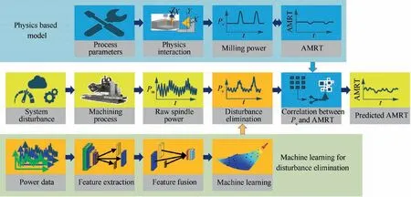
Fig.1 Framework of data-driven physics based model in dimensional accuracy prediction.

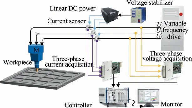
Fig.2 Measurement principle of spindle power.

As to the fF,8 features are extracted mainly based on the power spectral density(PSD)and shown in Table 2.Another frequency feature is extracted based on the frequency domain integration(FDI).PSD(f)is the power spectrum of power signal Pw(g).f1and f2are the passband cutoff frequency.

Apart from the abovementioned two types of features,the fT-Fare also extracted based on the wavelet analysis.According to the feature extraction in other research,db5 wavelet function is selected at the decomposition level three16.The sum of energy of all nodes in each level are calculated respectively and regarded as the fT-F.

For training the disturbance model,features are not the more the better,some features are redundant and will decrease the training accuracy.At the same time more features will reduce the calculation efficiency.Through correlation analysis,the features that have the high correlation with the Pd(g)can be finally determined17.

2.1.2.Feature fusion of power data

kPCA is a deep learning algorithm,and it is widely applied in feature fusion and extracting relevant information from complex nonlinear feature sets to reduce the redundancy among features19.The selection of kernel function and control parameter are crucial for the efficacy of kPCA.The common kernel functions contain poly kernel,rbf kernel and cosine kernel.

The feature matrix U is presented by Eq.(3).uk=[u1k,u2k,...,uik]represents the feature vector.k=1,2,...,K,and i=1,2,...,S.K and S denote the number of feature vector and feature,respectively.Because U contains various features,and the dimensions of each featured are different,U has to be prepossess via standardization.Projecting U to the high dimensional feature space,so the projected feature spaceΠ(U)is obtained and expressed by Eq.(4).

Mcovrepresents the covariance matrix ofΠ(U),its eigenvaluesγand eigenvectors H are given by Eq.(5).ξ=[ξ1,ξ2,...,ξk]Tis the weight vector.

Introducing the kernel function,the expression of kernel function matrix T is given:

where KERpcarepresents the kernel function,and the common kernel functions are given:

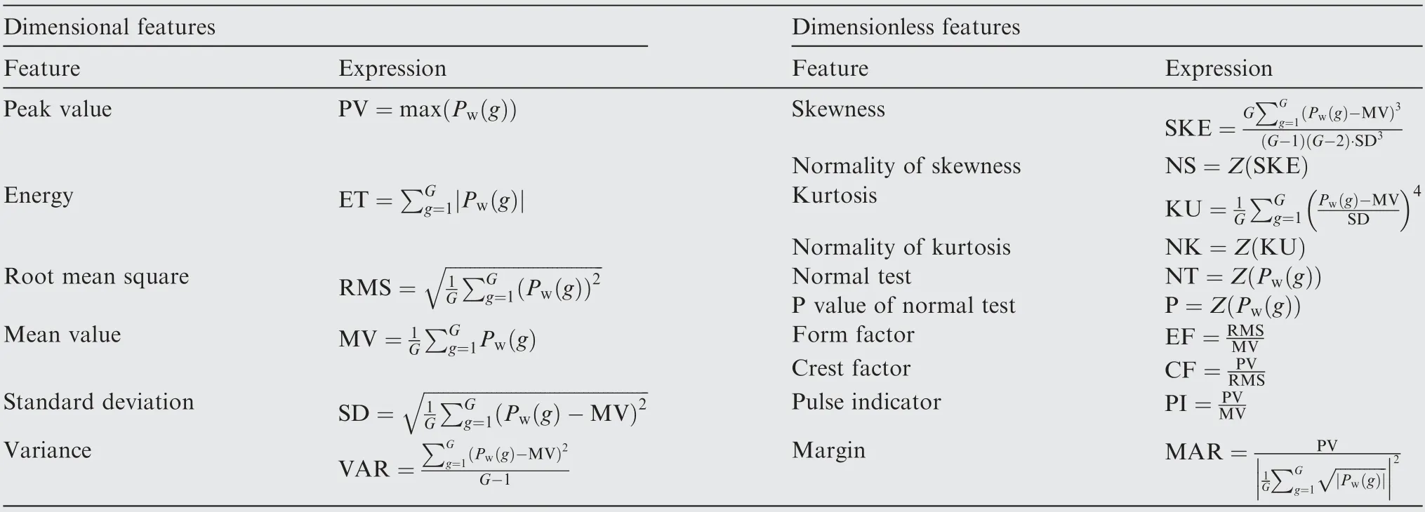
Table 1 Mathematical expression of fT.

Table 2 Mathematical expression of fF.

Finally,the kernel principal components space(feature fusion space)pc can be obtained and given by Eq.(8).

2.1.3.Construction of disturbance model

Kernel SVR(kSVR)is employed to construct the disturbance model Pd(g).kSVR is the derivation of SVM,and is a supervised machine learning algorithm based on the structural risk minimization20.kSVR trains the model based on the theory of classification.kSVR is applicable to deal with the problem of dynamic modeling of complex nonlinear system and modeling with smaller sample,and possesses the advantages of robust and good generalization21.The accuracy of the trained model is reliant on the selection of parameters and kernel function.

(pc,o)is the training sample,and pc is the input feature fusion space and given by Eq.(9).o is output variable and represented by Eq.(11).

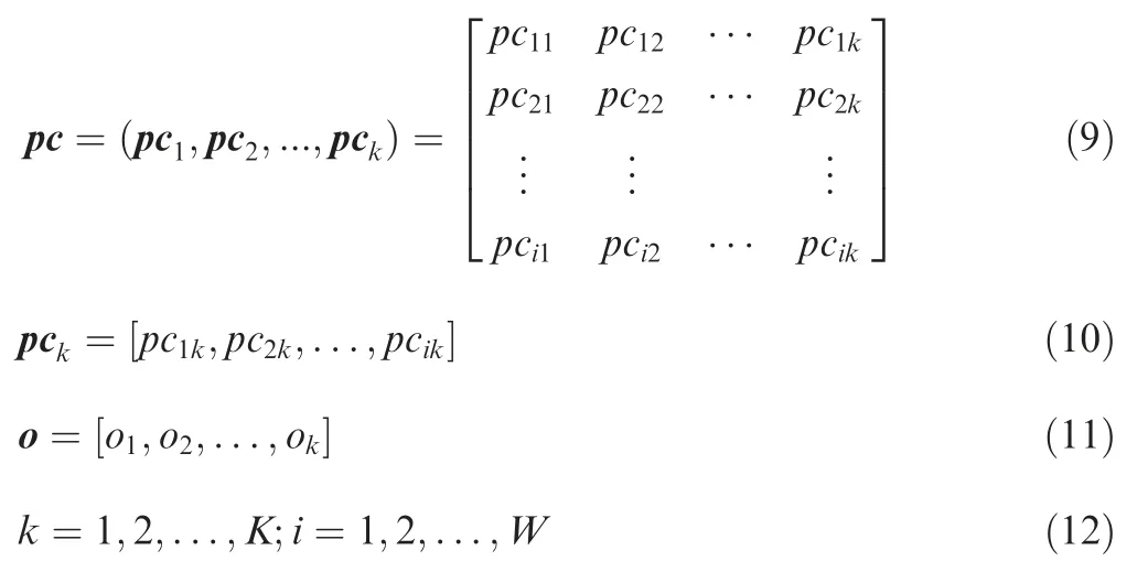
where pckrepresents the feature vector;K is the number of the feature vector;W denotes the number of principal component.The purpose of kSVR is to get an expression that satisfies the structural risk minimization.The expression is given as:

whereΓ(pc)is the nonlinear mapping of higher dimensional feature space of pc;σandεare the coefficients that need to be identified.In order to identifyσandε,Eq.(13)can be transformed into the form of solving minimization problem which shown as:

where C is the coefficient;leis loss function,and given by:

where e is the insensitive error.

The relaxation factorψandψ＊are introduced into Eq.(14),then Eq.(14)can be transformed into:

Then the Lagrange function can be obtained by introducing Lagrange multiplierμ,μ＊,βandβ＊and given by:

The dual problem of Eq.(18)is given by:

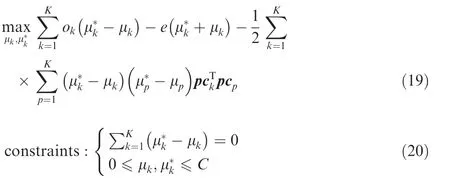
And Eq.(19)has to meet the Karush-Kuhn-Tucker conditions:

Taking the partial derivative ofσ,ε,ψkandψ*k with Eq.(18)and making the partial derivative equal to zero,then the following equations can be obtained:

Finally,the solution of SVR can be calculated:

where KERsvrrepresents the kernel function,and contains poly,rbf and sigmoid kernel,and is given:

where dkis order;c1,c2and c3are parameters,c1>0.

2.2.Physics based model for AMRT prediction

In rigid milling power model,the milling cutter is divided into a finite number of equal-thickness thin slices in the direction of cutter axis22.In Fig.3,dz=ΔZ/M is the element thickness,ΔZ is the AMRT and M is the number of slices along cutter axis.

{j,zl}represents the jth flute of the slice which distances from the bottom end of the cutter is zl.θj(zl)is the immersion angle of{j,zl}.zlis represented by

Assigning the bottom end of one flute as the reference immersion angleθ,thusθj(zl)can be represented as:

where N is the number of flutes;θpis cutter pitch angle and given by Eq.(28);zlkτrepresents the lag angle at the distance zl;kτis lag coefficient caused by the helix angleτ,and calculated by Eq.(29).

whereτis the helix angle of cutter;D is the cutter diameter.

The total forces acting on the cutter in the X and Y at immersion angleθare represented by

where dFQ(θj(zl))(Q=X,Y)denotes the forces acting on{j,zl}at the immersion angleθj(zl)in X and Y directions,and are presented by

where dFt(θj(zl))and dFr(θj(zl))denote the tangential and radial forces that act on{j,zl},and are given as:

where Ktc,Kte,Krcand Kreare cutting coefficients;h(θj(zl))is the rigid instantaneous uncut chip thickness(IUCT)of{j,zl},and is given by Eq.(33);q(θj(zl))is the window function of{j,zl}and given by Eq.(34).

where fcdenotes feed per tooth.

whereθstandθexdenote the entry and exit angle,respectively.For down milling,θstandθexare given by

where R is the cutter radius;rdis the radial depth of cut.

Based on the above equations,the milling power at immersion angleθcan be calculated in Eq.(36),and the average power of V revolutions can be calculated in Eq.(37).

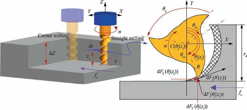
Fig.3 Rigid model of peripheral milling.

where vs=πDn denotes cutting speed,n represents rotation speed.

The correlation between the actual milling power and milling parameters are given by Eqs.(26)-(37).The AMRT ΔZ can be calculated when the average milling power Pc-aveand other milling parameters are given.The larger rd,ΔZ and fcwill cause the deflection of the milling cutter,thus the actual removed material deviates from the nominal removed material for a large extent,and ultimately the machining accuracy is decreased.The following content will embed the effect of cutter deflection into the rigid milling power model.

2.2.1.AMRT prediction during straight milling

In practical milling process,the milling cutter will deform along X and Y directions under milling force FQ(θ)(Q=X,Y),as shown in Fig.4.In order to investigate the mechanism of cutter deflection,the milling cutter is regarded as cantilever beam.In Fig.4,C(θj(zl))represents the desired cutter center of element{j,zl}at the immersion angleθj(zl),and C(θj-m(zl))represents the desired cutter center of element{j-m,zl}at the immersion angleθj-m(zl).Because of the cutter deflection,the desired cutter center C(θj(zl))and C(θj-m(zl))deviate from the cutter axis,and shift to the deformed center Cd(θj(zl))and Cd(-θj-m(zl)),respectively,as shown in Fig.4.m represents that the current cutter tooth is removing the material left by the previous mth cutter tooth,and m[1,N].Therefore,the IUCT considering cutter deflection which denoted by hd(θj(zl))will be different from Eq.(33).hd(θj(zl))is the radial thickness between the surface generated by{j-m,zl}and{j,zl}at the current immersion angleθj(zl),as shown in Fig.4.

hd(θj(zl))is calculated by

with

Through solving Eq.(39),u is given by

Thus,Eq.(38)can be substituted by

Because hd(θj(zl))≪R,hd(θj(zl))has the unique expression

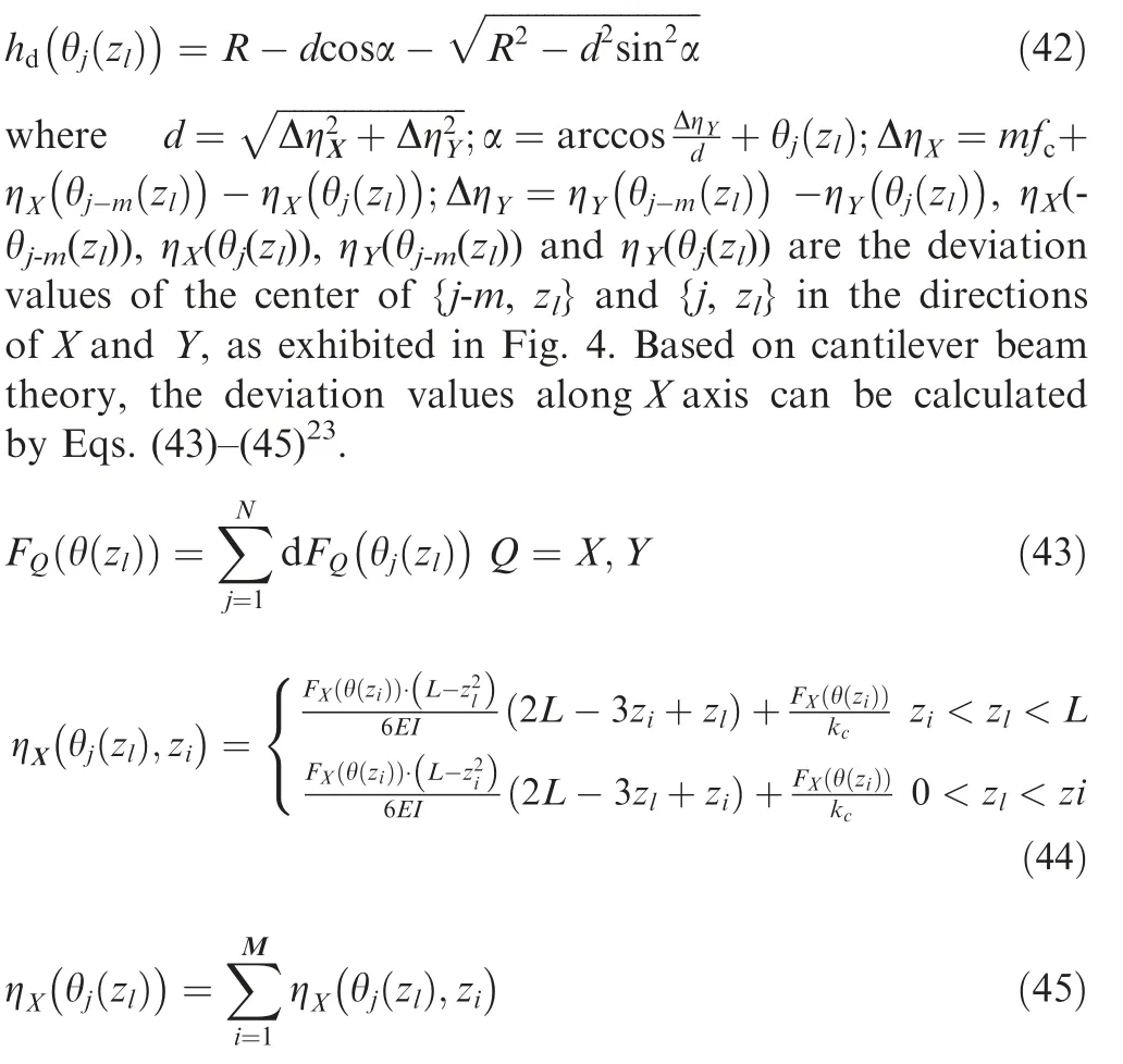
where ziis the element which distance from the bottom end of the cutter is zi;L denotes the over-hang;E represents the elastic modulus;ηX(θj(zl),zi)represents the deviation values of the center of{j,zl}along X axis caused by the forces acting on slice{zi};FX(θ(zi))denotes the cutting force acting on slice{zi}.kcrepresents the clamping stiffness and can be acquired via experiment;I represents the area moment of inertia and can be calculated by

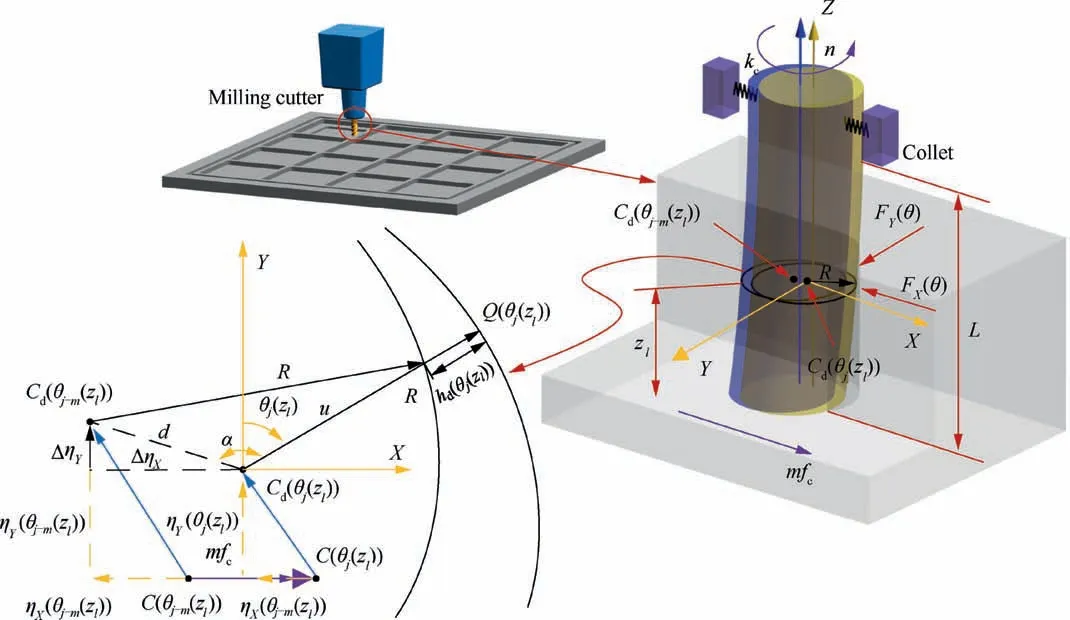
Fig.4 Cutter deflection.

where Rsis equivalent cutter radius and Rs=0.8R23,24.

The deviation values along Y axis can be acquired by replacing the subscript X of Eqs.(43)-(45)with subscript Y.

The IUCT that taking the cutter deflection along X and Y directions into account is expressed by Eq.(42).Eq.(42)contains both the cutter deflection and the clamping stiffness of collet.The deflection along X direction will affect the milling angle.For down milling,considering the deflection effect,the entry angle and exit angle are given as:

Substituting Eqs.(33)and(35)with Eqs.(42)and(47),respectively,the milling power model for straight milling by considering cutter deflection and clamping stiffness is established.Based on the established model,AMRT can be predicted when the average milling power Pc-aveand other milling parameters are given.

2.2.2.Material removal prediction during corner milling

The complete corner milling is divided into five stages from the start point C1to the end point C6,as shown in Fig.5(a),and during C3→C4stage,the milling cutter moves around toolpath center O with tool-path radius Rt.The trajectory of the point on the milling edge is epitrochoid.

The trajectory of point A on{j-1,zl}is given by Eq.(48).The trajectory of point B on{j,zl}is given by Eq.(49).

whereΘ(zl)denotes position angle along epitrochoid path of slice{zl}which distance from the bottom end of the cutter is zl;δrepresents the rotation angle of milling cutter around tool-path center O;Θ(zl)andδcan be calculated by Eqs.(50)and(52),respectively.

whereθpis cutter pitch angle and given by Eq.(28);z1denotes the first element.θ0is initial angle and set to 0;θis rotation angle;zland kτare calculated with Eqs.(26)and(29),respectively.κis calculated by

Therefore,ΘA(zl),δA,ΘB(zl),andδBat points A and B in Eqs.(48)and(49)can be calculated through Eqs.(50)-(52):

The trajectories of tool center of{j,zl}and{j-1,zl}are given as:

The IUCT without cutter deflection is given by

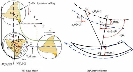
Fig.5 Corner milling.

In order to representΘA(zl)withΘB(zl),Ω(zl)is introduced and given as:

Through iteration algorithm25,and combining Eqs.(53)-(55),Ω(zl)can be obtained:

The tangential,radial forces that act on{j,zl}and{j-1,zl}are denoted by dFt(θB(zl)),dFr(θB(zl)),and can be calculated with Eqs.(31)and(57).dFX(θA(zl)),dFY(θA(zl)),dFX(θB(zl)),and dFY(θB(zl))are given as:

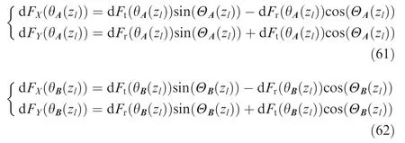
When the cutter deflection is considered,as exhibited in Fig.5(b),the trajectories of tool center of{j,zl}and{j-1,zl}are changed into:

whereηX(θA(zl)),ηX(θB(zl)),ηY(θA(zl))andηY(θB(zl))can be calculated with Eqs.(61),(62),and(42)-(44).

The trajectory of point A on{j-1,zl}is changed into:

Finally,the ICUT with cutter deflection of corner milling is given as:

The entry angle of corner millingθcstchanges with the milling position,and given by Table 3.Also,the cutter deflection is embedded intoθcst.The exit angleθcexisπ.

Substituting Eqs.(32)and(34)with Eq.(66)and theθcstin Table 3,respectively,the milling power model for corner milling by considering cutter deflection and clamping stiffness is built.Based on the built model,AMRT can be predicted when the average power Pc-aveand other milling parameters are given.

2.2.3.Numerical calculation of milling power model

Due to the cutter deflection,the milling power model will achieve convergence after multiple iteration.Fig.6 shows the iteration process of milling power model.During the iteration,the cutting force acting on slice zlalong X and Y direction FQ(θ(zl))(Q=X,Y)are calculated firstly based on the rigid IUCT.Then the deviation of each elementηX(θj(zl))andηY(θj(zl))which calculated though Eq.(44)are loaded to recalculate the IUCT and immersion angle,meanwhile the value of FQ(θ(zl))will be updated.The updated FQ(θ(zl))will also change the IUCT and milling angle.The FQ(θ(zl))will converge after multiple iteration,that is,the deflection of each slice and FQ(θ(zl))are balanced.The residual errorζis used to identify the convergence of FQ(θ(zl)),which is given by Eq.(67).In Eq.(67),FX(θ(zl),istep)represents the calculated FX(θ(zl))at the current step.After the iteration,the convergent IUCT can be output and used to calculated Pc-ave.

2.3.Development of data-driven physics based model

The flowchart of the data-driven physics based model is exhibited in Fig.7.The historical and real-time Pw(g)are obtained by eliminating the noise and idle power of the mea-sured power Pm(g).The features of fT,fFand fT-Fdomain of historical and real-time Pw(g)are extracted.With the selected features,the feature matrix[Uh,Ur]which combines features of historical and real-time Pw(g)is established.The standardization process is conducted on[Uh,Ur].After standardization,kPCA is used to deeply fuse the features of[Uh,Ur],and the principal component matrixΛ([Uh,Ur])is obtained.The first two principal component(pc1and pc2)of historical and real-time Pw(g)are extracted fromΛ([Uh,Ur]),respectively.The pc1and pc2of historical Pw(g)are regarded as input variable and fed into kSVR.The Pd(g)of historical Pw(g)is regarded as the output variable of training samples,and achieved by calculating the differences between the historical Pw(g)and the milling power Pc-ave(g)which calculated based on the milling power model with the historical AMRT.Through tuning the parameters of kSVR,the disturbance model can be constructed.The Pd(g)of real-time Pw(g)can be identified by feeding the pc1and pc2of real-time Pw(g)into the constructed disturbance model,so the real-time average milling power Pc-ave(g)can be obtained by Eq.(2).Finally,the AMRT can be predicted with the physical model and real-time Pc-ave(g).

Table 3 Expression ofθcst during complete corner milling.

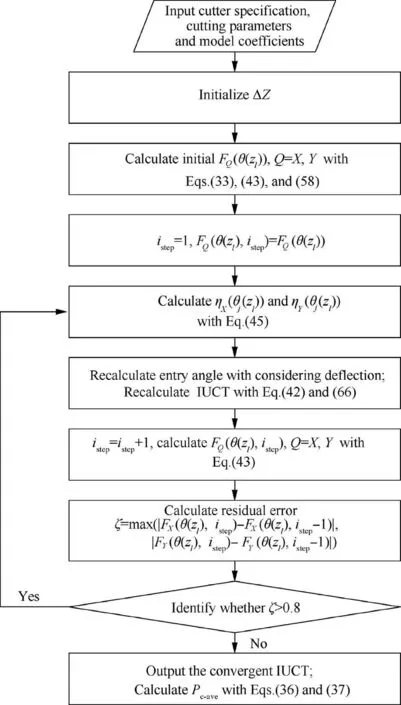
Fig.6 Iteration process of milling power model.

3.Experimental verification and results analysis

3.1.Coefficients determination of physics based model

The coefficients Ktc,Kte,Krc,Kreare determined through implementing a series of slot milling experiments26.The workpiece material is Al-2219 alloy.A cylindrical end mill is used and its specification is exhibited in Table 4.The experiment is carried out on DMG milling center.The identified Ktc,Kte,Krcand Kreare 787.229 N/mm2,35.597 N/mm,344.686 N/mm2and 93.471 N/mm,respectively.The clamping stiffness kcis measured to be 1.76×107N/m.

3.2.Comparison for calculated and experimental milling power

The milling power is extracted from the measured power which acquired from a practical pocket milling operation.A thinwalled Al-2219 alloy plate is used as the workpiece,and its dimension is 500 mm×500 mm×18.5 mm.The machining parameters of pocket milling are given in Table 5.

The pocket milling operation is exhibited in Fig.8(a).The AMRT is obtained through calculating the coordinate difference along Z direction before and after milling,and the coordinate values along Z direction are measured by the probe of machine-tool,as shown in Fig.8(b).The spindle power measurement system is shown in Fig.8(c).The sampling frequency is set to 50 kHz.Before analog-to-digital conversion,the antialiasing filter with 10 kHz is set to avoid frequency-band overlapping.The power and AMRT data of the second layer are measured to verify the proposed method.

The tool path and measurement position of AMRT for each pocket is exhibited in Fig.9.The measured power and corresponding AMRT of the first pocket are shown in Fig.10(a).By matching power with tool path,the tool path and corresponding power are exhibited in Fig.10(b).The Pn(g)of the power that shown in Fig.10 is eliminated by low pass filter of 250 Hz.The Piof the power that shown in Fig.10(b)is removed.The 80 sets of Pw(g)and measured AMRT of the first four pockets are regarded as the historical data and used to train the disturbance model.Each Pw(g)consists of 9000 power data points(15 revolutions)which center on the measurement position.The 56 sets of data are employed to train the disturbance model in straight milling,and 24 sets of data are employed to train the disturbance model in corner milling.The power data from each verification pocket is separately inputted into the proposed method to predict AMRT.The rbf kernel function and poly kernel function are selected to construct the disturbance model in straight and corner milling,respectively.

Fig.11 shows the comparison for the calculated and experimental average milling power in the straight milling of the first pocket.In Fig.11(b),the calculated Pc-ave(g)-flex and Pc-ave(g)-rig are the average power of 15 revolutions,and achieved based on the flexible and rigid milling power model,respectively.The AMRT is measured from the first pocket.In Fig.11,the experimental average milling power Pc-ave(g)-MFML is obtained by eliminating the disturbance of the average Pw(g)with multi-feature fusion machine learning(MFML)and flexible model.The max error between the Pc-ave(g)-flex and average Pw(g)is 223.782 W,while the max error between the Pc-ave(g)-flex and Pc-ave(g)-MFML is just 2.51 W.

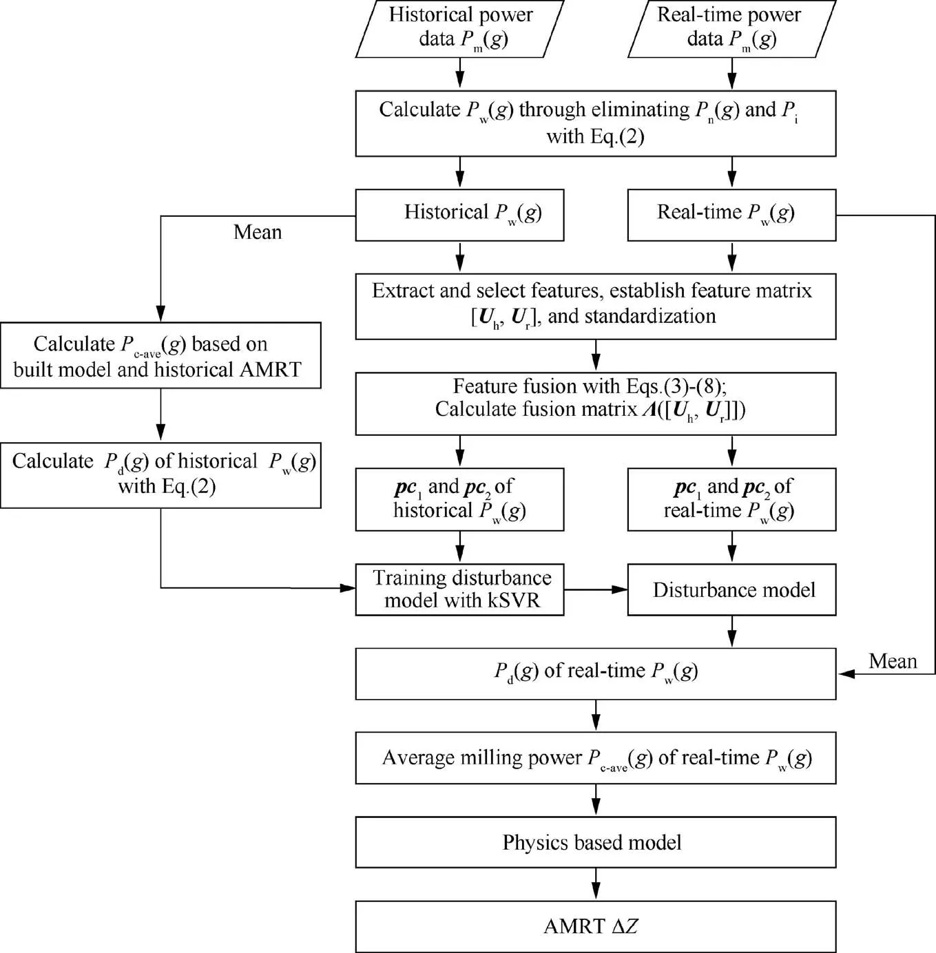
Fig.7 Flowchart of data-driven physics based model.

Table 4 Specifications of cylindrical end mill.

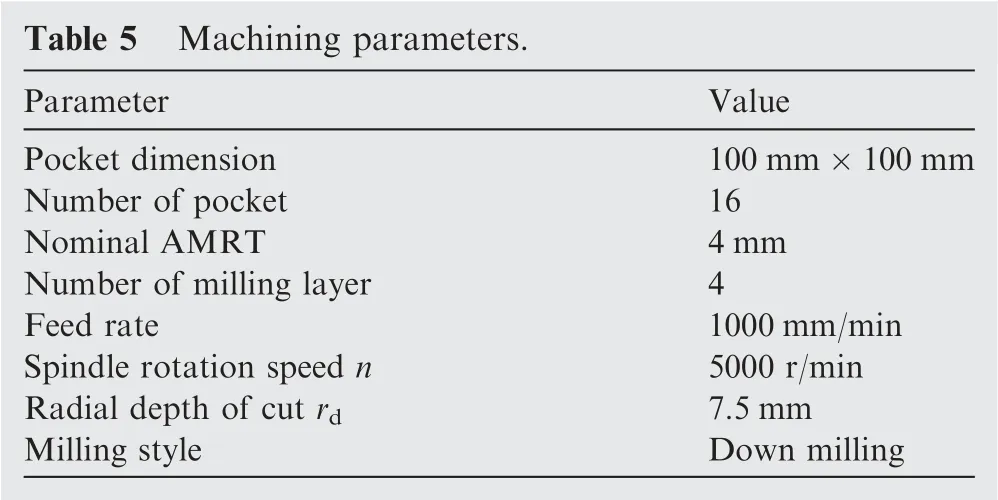
Fig.12 shows the comparison for the calculated and experimental average milling power in the corner milling of the first pocket.In Fig.12(a),the complete corner power Pw(g)is obtained from one of the first pocket,and the average Pw(g)is calculated with per 15 revolutions of power data.In Fig.12,the calculated Pc-ave(g)-flex and Pc-ave(g)-rig are theaverage power of 15 revolutions,and simulated based on the flexible and rigid corner power model,respectively.The AMRT that used to simulate the complete corner power is 4 mm,and the AMRT that used to calculate Pc-ave(g)-flex and Pc-ave(g)-rig is measured from the first pocket.In Fig.12(b)and(c),the max error between the Pc-ave(g)-flex and average Pw(g)is 299.971 W,while the max error between the Pc-ave(g)-flex and Pc-ave(g)-MFML is just 1.099 W.

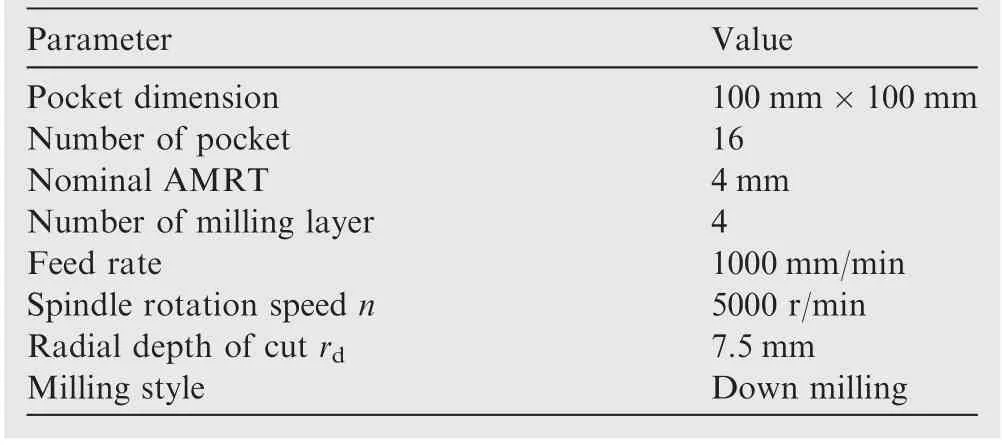
Table 5 Machining parameters.

3.3.Analytical expression of the correlation between power and AMRT

The built milling power model has provided the correlation between AMRT and Pc-ave.The Pc-averepresents the average power of 15 revolutions.Because the cutter deflection and clamping stiffness are considered into the flexible model,the deflection iteration in the built model will consume a lot of time.In order to improve the predicted efficiency,the analytical expression of the correlation between Pc-aveand AMRT is fitted based on the built model.

Fig.13 shows the correlation between Pc-aveand AMRT.The range of AMRT is 2 mm to 8 mm.The increment of power error between the rigid and flexible power model increases with AMRT.As shown in Fig.13,the correlation between Pc-aveand AMRT is approximately linear when AMRT varies between 3.8 mm and 4.2 mm.The flexible analytical expression of straight and corner milling are given by Eqs.(68)and(69),and max error of Eqs.(68)and(69)are 0.001 mm and 0.002 mm,respectively.The rigid analytical expression of straight and corner milling are given by Eqs.(70)and(71),and the max error of Eqs.(70)and(71)are 0 mm and 0.001 mm,respectively.

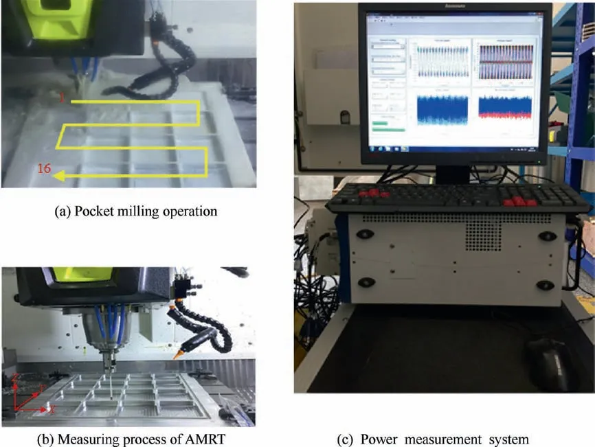
Fig.8 Experiment setup.

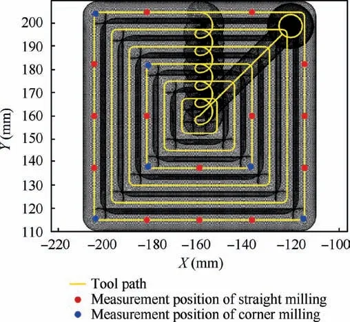
Fig.9 Tool path and measurement position.

3.4.Prediction accuracy of the proposed method

Fig.10 Tool path and corresponding power and AMRT.

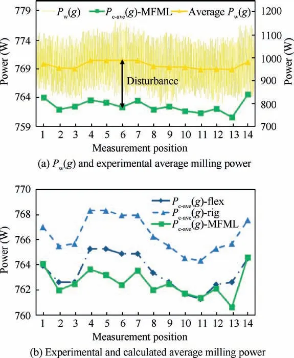
Fig.11 Experimental and calculated average milling power in straight milling.

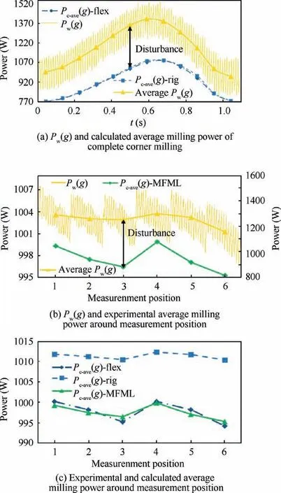
Fig.12 Experimental and calculated average milling power in corner milling.

Pockets 5,6,8,12,and 16 are selected based on the heuristic knowledge of engineer and the even distribution on the time series distance to verify the accuracy and effectiveness of the proposed method.To verify the efficacy of MFML for eliminating the disturbance,comparison experiments are conducted with traditional response surface methodology based(RSM),time domain feature fusion machine learning(TFML)and single feature machine learning(SFML).To verify the prediction accuracy of the flexible milling power model,comparison experiment is implemented with the rigid model based multifeature fusion machine learning(MFML-rig).In addition,the AMRT is also predicted through the proposed datadriven physics based model but without eliminating disturbance(WED)to illustrate the effect of the disturbance.The implementation details of the comparison experiments are given in Table 6.Multi-feature fusion trains the disturbance model through the fusion of time domain,frequency domain and time-frequency domain features.

The power data of pocket 12 and 16 after eliminating the disturbance through different disturbance elimination method are given in Fig.14.The average milling power Pc-ave(g)-rig is calculated through eliminating the disturbance from average Pw(g)with the multi-feature fusion machine learning and the built rigid power model.Through inputting the calculated Pc-ave(g)-rig into Eqs.(70)and(71),the AMRT can be predicted through MFML-rig.For predicting AMRT by WED,the average Pw(g)is directly inputted into Eqs.(68)and(69)without eliminating the disturbance.The power values of the measurement position with the max prediction error of AMRT in straight and corner milling stage are marked in Fig.14.

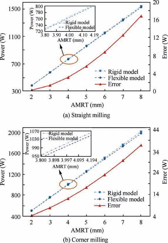
Fig.13 Correlation between average milling power and AMRT.

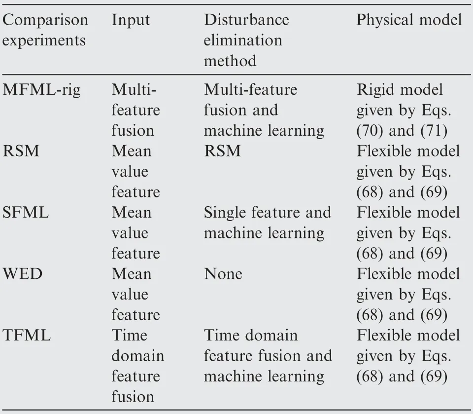
Table 6 Implementation details of the comparison experiments.

The max error of verification results are given in Fig.15.It can be seen from the comparison results,the MFML with the built deflection model performs better.The max error in straight and corner milling are 0.014 mm and 0.019 mm,respectively.The max error of MFML-rig is just 0.005 mm more than MFML.The reason for that is the disturbance elimination through multi-feature machine learning can also eliminate the deflection disturbance of cutter.The max error of WED in straight milling and corner milling are 1.199 mm and 1.333 mm,respectively.Compare MFML and WED,the disturbance in the power data greatly decreases the calculation accuracy of the physical model.The disturbance power is mainly consumed on the wire resistance and friction(machine tool system and cutting process).On the contrary,the proposed multi-feature fusion and machine learning can effectively eliminate disturbance and improve the predicted accuracy of the physical model.The comparison among MFML,TFML and SFML proves the advantage of the multi-feature fusion in eliminating the disturbance,and the disturbance(including the disturbance induced by the measurement error)can be further eliminated with the fusion of multiple features.The reason for that is the multi-feature fusion can improve the ability of disturbance identification of the proposed data-driven physics based model,and the disturbance can be eliminated adequately.The tool path and AMRT that predicted via MFML of pockets 5,6,8,12 and 16 are exhibited in Fig.16.

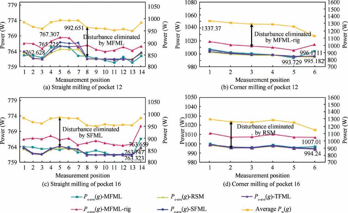
Fig.14 Power data after eliminating disturbance through different method.

Fig.15 Comparison of max error.

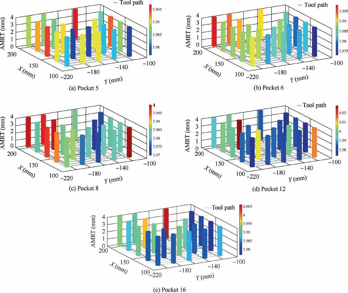
Fig.16 Predicted AMRT and corresponding tool path position.

4.Conclusions

In this paper,the framework of data-driven physics based model is proposed and developed for the real-time prediction of AMRT,which determines the RBTE of pocket components.The physics based model considers the primary root cause,in terms of tool deflection and clamping stiffness induced AMRT variation.In order to eliminate the disturbance caused by the dynamic and inherent coupling of the complicated manufacturing system,the disturbance model are constructed based on the features of the power data with kPCA and kSVR,and incorporated with the physics based model.Therefore,the proposed data-driven physics based model combines both process mechanism and the system disturbance to achieve better prediction accuracy.The accuracy and effectiveness of the proposed method are proved by the verification experiment.The prediction accuracy of AMRT achieves 0.014 mm and 0.019 mm for straight and corner milling,respectively.Therefore,the proposed method can assist the engineers to determine the compensation strategy to control the final RBTE.The multi-feature fusion and machine learning can effectively eliminate the disturbance and greatly improve the predicted accuracy of the physical model.The comparison with RSM,SFML and TFML proves the advantage of the multi-feature fusion and machine learning.The deflection model can further improve the prediction accuracy which is proved by comparing with MFML-rig.

Declaration of Competing Interest

The authors declare that they have no known competing financial interests or personal relationships that could have appeared to influence the work reported in this paper.

Acknowledgements

This research is supported by the Science and Technology Major Project of China(No.2019ZX04020001-004,2017ZX04007001).