Quantitative assessment and visualization of flight risk induced by coupled multi-factor under icing conditions

Yang WEI, Haojun XU, Yuan XUE, Xiaocong Duan

School of Aeronautics Engineering, Air Force Engineering University, Xi’an 710038, China

KEYWORDS Flight risk;Icing;Multivariate extreme value theory;Quantitative assessment;Visualization

Abstract Aircraft icing has been proven to be one of the most serious threats to flight safety.During the analysis of flight risk under icing conditions, quantitative assessment and visualization of flight risk are quite essential as they provide safe manipulation strategies in intricate conditions.However, they are rarely studied. Since the icing flight accidents are the result of the coupling of multiple unfavorable factors,in present study,we have proposed a method to quantitatively assess flight risk induced by multi-factor coupling under icing conditions by Monte-Carlo simulation and multivariate extreme value theory.The results demonstrate that the flight risk probability increases with the rise of unfavorable factors. Besides, a flight risk visualization method named flight safety window has been presented to build the flight risk distribution cloud maps in different complex conditions.The cloud maps show that the icing would give rise to atrophy of the safety scope,and the consequence would be even more severe when coupled with other more unfavorable factors. The proposed methods in this study would be useful in flight risk analysis under icing conditions and can enhance the pilot’s situational awareness in selecting correct strategies within the safety zone to avoid unsafe manipulation.

1. Introduction

Loss-of-Control (LOC) is a major contributor to flight accidents.1In a recent NASA statistical analysis of LOC accidents,aircraft icing has been proven to be one of the most common external environmental LOC causal factors.2Accidents caused by icing happen sometimes.According to the accident statistics of National Transportation Safety Board (NTSB), there were 565 icing-related flight accidents from 1998 to 2007, leading to the death of 229 people.3The occurrence of flight accidents usually is the coupling result of multiple unfavorable factors within the Pilot-Aircraft-Environment(PAE)complex system.One of the possible multi-factor coupled flight risk event chains under icing conditions is shown in Fig. 1, where we can see that the aircraft enters a more and more dangerous situation since these adverse factors happened one by one.

Icing affects the aerodynamic characteristics, control and stability characteristics of aircraft. Excessive ice accretion on the lifting surface would change the aerodynamic configurations of the lifting surfaces, making the lift decrease and drag increase.4Simultaneously, the stall speed would reduce and stall angle of attack would increase. Afterwards, the aircraft will enter an unexpected stall state under icing conditions more easily,which will even cause devastating disasters like the Colgan Air Flight 3407 accident in 2009.5Ice accretion on the main aircraft control surface may cause the loss of control effectiveness, and even the control surfaces jammed in some severe cases.The severe accident example is that the American eagle flight 4184 crashed during a rapid descent after an uncommanded roll excursion because the aileron lost the control effectiveness caused by icing.6

The sensors equipped in aircraft such as the airspeed tube and the angle of attack sensor provide the necessary input parameters for the pilot and flight control system to control the airplane. The fault of sensors may occur due to ice accretion,affecting pilot’s judgment of the aircraft states.Recently,a Boeing 787MAX aircraft of Ethiopian Airlines crashed in March 10, 2019. One of the reasons for the accident was considered to be a failure of the angle of attack sensors.

Aircraft icing has been deemed as an ongoing threat to aviation safety7and attracted a lot of attentions of researchers.At present, the researches on aircraft icing mainly focus on the aerodynamic characteristics,8-13flight dynamic characteristics,14-18and envelope protection.19-23The quantitative probability of flight risk is a key reference index, which is vital in decision making regarding the flight safety of PAE complex system. However, in the previous studies about flight risk assessment under icing conditions, only the single factor was involved. For example, only the flight risk assessment under the aerodynamic effects of icing24is taken into consideration without the influence of multiple factors such as aerodynamic deterioration, reduced control effectiveness of control surface,and the sensor failure caused by icing. Therefore, in-depth studies on icing flight risk assessment under the coupling of multi-factor are quite eagerly needed.

The conventional system security design generally follows the methods recommended in SAE ARP 4761,25SAE ARP 4754,26MIL-HDBK-516B,27MIL-STD-882E28as well as other safety specifications. Commonly, most of these methods calculate the probability of flight accidents based on the original internal hardware system failure rate; however, quantitative indicators for the dynamic flight risk induced by the external environmental factors are lacking. Model-Based Systems Engineering(MBSE),a series of modified ideas,provides a possible solution for the flight risk quantitative assessment of the PAE complex system.In other words,we are able to combine modeling and simulation methods to assess the flight risk with multi-factor quantitatively by adopting the idea mentioned above.

Meanwhile, the visualization method of flight risk29-32is a hot topic in the researches of aviation field.However,there are few studies on the visualization of the flight risk for in-flight icing conditions, and unable to provide an intuitive indication and alarm for the pilot to manipulate the aircraft safely.Therefore, the quantitative assessment on flight risk under multifactor coupling,with an effective visualization,is sorely needed for flight safety.

In the present study, we have proposed a quantitative assessment method of flight risk induced by coupled multifactor under icing conditions based on Monte-Carlo simulation and multivariate extreme value theory. And a visualization method of flight risk named flight safety window is presented to build the flight risk distribution cloud map. To better illuminate this paper’s theme, the modeling of PAE complex system under icing conditions is first presented in Section 2, and the real-time flight simulation platform is constructed. Then the process of extracting extreme parameters based on Monte-Carlo simulation is presented, the credibility is verified,and the extreme value of safety critical flight parameters is calculated in Section 3. In Section 4, the distribution characteristics of extreme parameters are analyzed and a multivariate Copula model is presented to calculate the flight risk.In Section 5, the safety window calculation algorithm is proposed, and the safety cloud maps in different conditions are built. Finally, conclusions are drawn in Section 6.

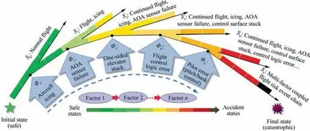
Fig. 1 Multi-factor coupled flight risk event chain under icing conditions.

2. PAE complex system simulation model and platform

2.1. PAE complex system simulation model

2.1.1. Pilot model

The typical pilot model structure is shown in Fig. 2.33. The four modules in the dotted box form the modeling of the pilot’s main behavioral characteristics, and the description of each module is shown as follows.

(1) Display including observed noise

The observation error is introduced by the pilot when the measurements from the displays are observed.

(2) Reaction time delay

There is uncontrollable minimum response delay time for the pilot to read signals,transmit them to the brain,and make decisions in the brain. e-τsis commonly used to indicate the delay link, and τ is typically in the range of 0.15-0.3 s.

(3) Compensation system

The compensation maneuver is equivalent to the controller in the feedback control system and is the core of the pilot model. To simplify the model, the feature can usually be represented by a static control gain Kp.

(4) Neuromuscular dynamics system

When the muscle receives the instructions from the brain,it presents the neuromuscular time-delay characteristics owing to its inertia, viscosity and the contraction. The feature can be represented by a first-order differential link 1/(TNs+1). The values of TNare about 0.1-0.2 s.

The observation noise and the noise signal during the operation have little effect on the dynamic simulation results. To simplify the calculation properly, it is ignored in the paper.Therefore, the pilot model can be expressed as

2.1.2. Aircraft dynamics model

A typical jumbo jet transport aircraft is used in this study,and the aerodynamic data can be found in Ref.34.The six-degreeof-freedom (6-DOF) nonlinear dynamic model of the aircraft can be expressed by the vector form of the following equation35:

where V, α and β are the flight speed, the angle of attack, and the side slip angle, respectively; q0, q1, q2and q3are quaternions,and q02+q12+q22+q32=1;p,q and r are the components of the angular velocity in the body coordinate system;xg,ygand zgare the positions of the aircraft in the ground coordinate system; δthis the throttle setting; δe, δaand δrare the elevator deflection angle, the aileron deflection angle and the rudder deflection angle, respectively.

The attitude angle of the aircraft, such as the roll angle φ,the pitch angle θ and the yaw angle ψ, can be obtained by quaternion transformation.

2.1.3. Flight control fault model

If the icing causes the sensor failure or the control surface to be jammed,it will affect the normal work of the flight control system. Therefore, it is necessary to establish a typical flight control system fault model. In this work, only sensor failures and actuator failures are studied.

(1) Sensor fault model

Define youtand yinas the actual and the normal output of the sensor,respectively,and three types of failure model can be expressed as

where a is a const, k1is proportional coefficient, and Δ is the deviation.

(2) Actuator fault model

Given uoutand uinas the actual and the normal output of the actuator, respectively, and two types of failure model can be indicated as

where b is a const, and umin≤b ≤umax. k2is the damage proportional coefficient of the control surface, and 0 ≤k2≤1.

Fig. 3 Longitudinal control law structure of fly-by-wire system with fault model.

(3) Flight control system

Taking the longitudinal flight control system of aircraft as an example, the control law structure of the typical civil aircraft longitudinal fly-by-wire control system is explained in Fig. 3. The whole control law structure can be roughly composed of a pitch command generation module, a maneuver command feedback module, a control augmentation module,an envelope protection module, a forward channel module and an actuator command generation module. It can be seen from Fig. 3 that the AOA is the key input parameter of the flight control system.Once the AOA sensor is faulty,the flight control system will make a wrong judgment. As the elevator deflection angle is the output of the longitudinal flight control system, a threat to flight safety will be posed because of the jammed elevator.

2.1.4. Icing aerodynamic effect model

The aerodynamic model of the icing aircraft is determined using the icing factor method,36and the expression is presented as

where η is the aircraft icing severity factor; KArepresents the variation in an aircraft parameter;CAis any arbitrary aerodynamic derivative of the clean aircraft;CA.icedis its value under the icing condition.

According to NASA research results,37a simplified icing aerodynamic effect model is built in this study, namely,

where t0is the initial time of icing; tmaxis the total time for icing.

2.2. Flight simulation platform

Through the LINKS-RT flight simulation platform as shown in Fig. 4, the simulation system module built by MATLAB/Simulink can be converted into the C++ code supported by the real-time system VXWORKS for real-time flight simulation.

3. Extraction process of extreme parameter and flight risk definition

3.1. Extraction process of extreme parameters based on Monte-Carlo simulation

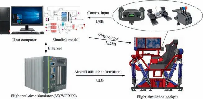
Fig. 4 Flight simulation platform.

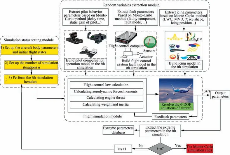
Fig. 5 Extraction process of key safety flight parameters’ extreme values.

As known, the process of multi-factor coupling induced flight risk under icing conditions is quite complicated, which is mainly reflected in the following aspects: (A) complex nonlinearity in the mathematical analysis model of the pilot and the aircraft; (B) different external environment, the pilot’s manipulation,and random occurrence of the fault.While the risk of encountering icing under intricate conditions is being studied,it is found that the randomness of internal and external factors requires a large amount of data, and flight test data cannot meet the data requirements.At the same time,the typical fault conditions of the flight control system,such as the jamming of control surface and sensor bias caused by icing,are difficult to be simulated through experiments. So here, the Monte-Carlo method has been adopted to solve randomness in the simulation process.The extraction process of key safety flight parameter extreme values is proposed as shown in Fig. 5.

The basic flow of extracting the extreme values of the flight parameters based on the Monte Carlo method is described below:

(1) Simulation status setting: set the aircraft body parameters and initial flight state, and set the number of simulation iterations. Here, define i=1.

(2) The extraction of random variables: extracting the pilot’s manipulation behavior parameters(the static gain Kp, delay time τ, and muscle delay time TN) in the ith simulation in the pilot database by using the Monte-Carlo method.

Base on this method, the icing severity, the ice shape and icing position parameters are extracted from the icing database to obtain the influence of icing on the aerodynamic forces and aerodynamic moments of the aircraft.

Then, the typical fault components (the sensor, the main control surface), the fault modes (such as sensor failure, the single-sided elevator / aileron jamming, the rudder jamming,etc.), and the fault model parameters of the flight control system will be extracted.

(3) Flight simulation: based on the extracted random variable parameters which have been confirmed in Step(2), the PAE system model of the ith simulation is constructed. A fourth-order Runge-Kutta differential algorithm is used to calculate the aircraft’s 6-DOF nonlinear Eq. (2), and the flight parameters of the aircraft in the simulation time domain are obtained. The time step for the differentiation is 20 ms.

(4) After extracting the extreme sample data of the key safety parameters in the ith flight simulation calculation,the data will be stored in the extreme value parameter database.

(5) Given i=i+1, return to Step (2). Continue the iterative simulation until i=n,and the Monte-Carlo simulation ends. n is the total number of Monte Carlo calculations.

In this study, we take the study of the longitudinal flight safety under icing conditions as a case,so the selected unfavorable factors are mainly concentrated in the longitudinal channel of the aircraft.

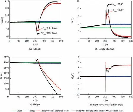
Fig. 6 Simulation results under the effect of unfavorable factors.

The simulation condition is set as follows:the aircraft is initially trimmed at a height of 3000 m with a velocity of 120 m/s.Entering the icing area, and starting icing, the icing severity parameter is assumed linear varying from η=0 at t=0 s to η=[0.1, 0.3] at t=300 s. After 5 min, an offset fault of the AOA sensor occurs with a range of [-5°, 5°], and the onesided elevator is jammed with the jammed angle range being[-15°, 15°]. Here, the total number of Monte-Carlo simulations is 3000.

The simulation results under the effect of unfavorable factors are shown in Fig. 6. In this simulation, the jammed angle of the left-side elevator is -10° and the offset value Δ of the AOA sensor is -5° with the icing severity factor η being 0.3.The pilot delay time τ is 0.2 s with muscle delay time TN=0.2 s.

From Fig.6,we can see that the aircraft height drops under icing conditions (Fig. 6 (c)) while the speed increases during the icing time (Fig. 6 (a)). Because the lift decreases and drag increases,the AOA increases in the icing time(Fig.6(b))in order to maintain sufficient lift.In the 300 s,when the left elevator is jammed at-10°,the pilot tries to use the right elevator(Fig.6(d)) to control the aircraft and correct the pitch attitude after the reaction time.However,the AOA and the speed have already been closed to the left boundary during the correction process.Coupled with the AOA sensor fault,the minimum velocity drops and the maximum AOA increases.Based on this trend,we can know that the aircraft starts to enter a more dangerous situation,as these unfavorable factors happened one by one.

Based on the simulation results, the AOA and airspeed are easily overrun parameters under icing conditions whose drastic change will lead to significant impacts on flight safety.Therefore, it is appropriate to choose the AOA and velocity as the key flight parameters to be extracted with the extreme values.

3.2. Credibility verification of extreme flight parameter and flight risk definition

Practically, it is impossible to perform 3000 times of flight tests. Furthermore, in some dangerous conditions, the real pilot in-the-loop ground simulation experiments are the only way to verify the credibility of the extracted extreme parameters using Monte-Carlo simulations. Besides, too many times of pilot in-the-loop ground simulations are difficult to carry out. Therefore, in the present study, the real pilot in-the-loop ground simulation experiments have been performed 300 times.

The scatter distributions of 300 extreme samples of simulation, the test data and the Quantile-Quantile (QQ) plots of simulation and test data are shown in Fig. 7. As can be seen from Fig.7(b)and(c),the QQ plots of the two extreme parameters (airspeed and AOA) are almost straight lines, indicating that the extracted extreme parameters and the test data belong to the same type of distribution, which demonstrate that the Monte-Carlo simulation data samples can be used to evaluate the flight risk probability.

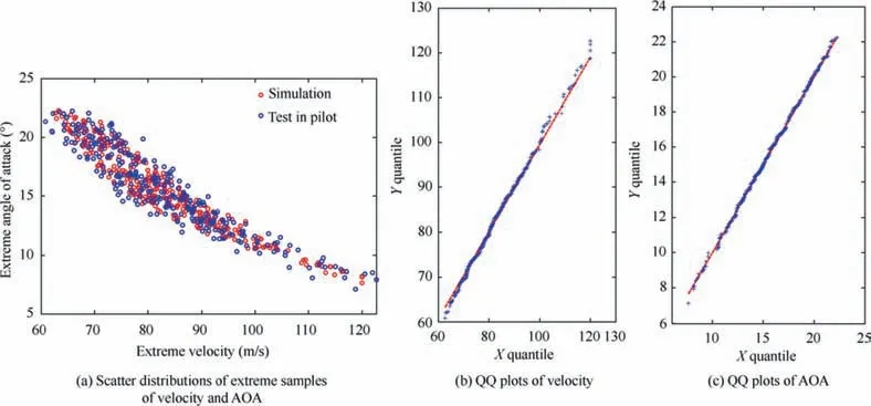
Fig. 7 Verification for the same distribution type of flight simulation data and test data.

where Vminand Vcare the extreme value of velocity and stall speed, respectively; αmaxis the extreme value of AOA; αcis the stall AOA which is the function of flap deflection angle δf, Mach number Ma and the icing severity factor η.

4. Distribution characteristics of extreme flight parameters

4.1. Distribution characteristics of one-dimensional extreme flight parameters

The values of the flight parameters(the median,variance,kurtosis, and skewness) of the one-dimensional extreme samples(Vmin, αmax) under icing conditions from statistical analysis performed by Monte-Carlo simulation are listed in Table 1.From Table 1,we can observe that the values of kurtosis coefficients on extreme velocity and AOA are both above 3, indicating that the extreme value samples of these two parameters behave with the characteristics of heavy tails compared with that of normal distribution.

Based on the results obtained above, the characteristics of various extreme value distribution models such as Generalized Extreme Value (GEV), Normal (Norm), Lognormal (Log),Weibull,Exponential(Exp),and Extreme Value(Ev)distributions are all studied here. These models are often used to describe the data that has heavy-tailed distribution features.The expressions of the six models are presented as follows:

GEV distribution:

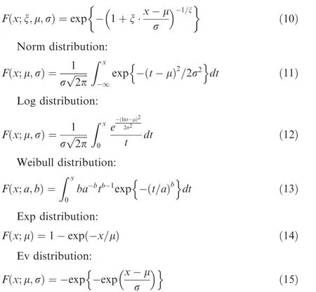
where ξ, μ, σ, a and b are the unknown parameters needed to be identified.

In this study, the unknown parameters in the six models used in our simulations are identified by the nonlinearidentification algorithm.The results are shown in Table 2.The probability density graph and the cumulative probability graph of extreme velocity and AOA are shown in Fig. 8 (a)and (b). From Fig. 8, we can see that the GEV distribution model and the Norm distribution model are more suitable to describe the distribution characteristics of one-dimensional flight extreme parameter. Besides, the K-S, A-D and χ2test methods are utilized to check the goodness of fits for the six models, as listed in Tables 3 and 4. From the listed values,we can know that the K-S test value of both GEV and Norm distributions is both less than 0.1, and P value of them is greater than 0.05 at a confidence level of 95%. P value of GEV distribution is far greater than that of other distributions,while A-D and χ2test values of GEV are the smallest among that of six distributions. Based on the analysis above, the GEV model shows the best fit to the extreme samples.

Table 1 Statistical characteristics of extreme value samples.

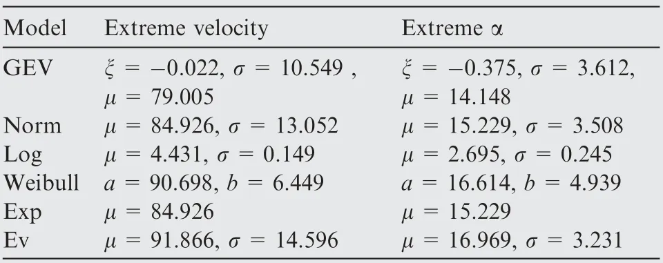
Table 2 Identified parameters based on different models.

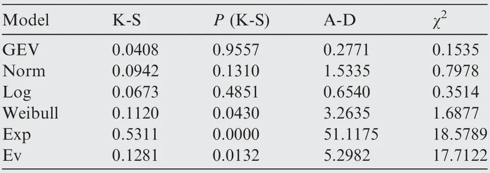
Table 3 Goodness of fit test of extreme Vmin.

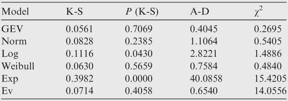
Table 4 Goodness of fit test of extreme αmax.

According to Eq.(9)and the identified GEV model parameters,the occurrence probability of flight risk can be expressed as

In accordance with the formulas above,the probabilities of flight risk calculated by minimum velocity and maximum AOA are 0.0974 and 0.0793,respectively.Both of them have reached the B level, namely, ‘‘possible”, which is in line with the MILSTD-882D. The results indicate that the probabilities of flight risk obtained from different parameters are different in the same simulation case.Thus the flight risk calculated by a single parameter is not comprehensive. Usually, the occurrence of flight risk is associated with deterioration of multiple flight state parameters.

4.2.Flight risk calculation based on multivariate Copula models

The one-dimensional extreme distribution has been identified above. Nevertheless, according to Eq. (9), the determination of the flight risk under icing conditions involves the correlation structure of the two-dimensional extreme parameters. The joint distribution of multi-dimensional variables is concerned with the edge distribution of each variable, and the relationship between the variables are more important. When the number of random variables is large,the extreme behavior of a single variable does not contain the joint extreme behavior of the entire variables. In this paper, the Copula theory38is applied to model the correlation structure in multidimensional extreme parameters.

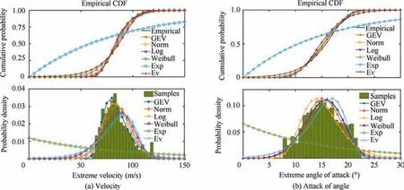
Fig. 8 Probability density graph and cumulative probability graph of extreme parameters.

According to Fig.7(c),the extreme AOA has lower tail distribution characteristics while the extreme velocity has upper tail distribution characteristics.In order to build the multivariate Copula model,the extreme velocity Vminis converted as the extreme relative velocity V-max:

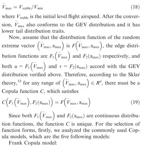
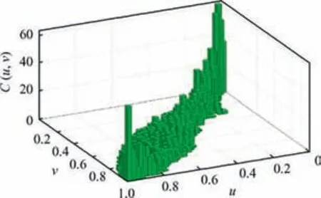
Fig. 9 Joint probability distribution histogram of two-dimensional extreme parameters.

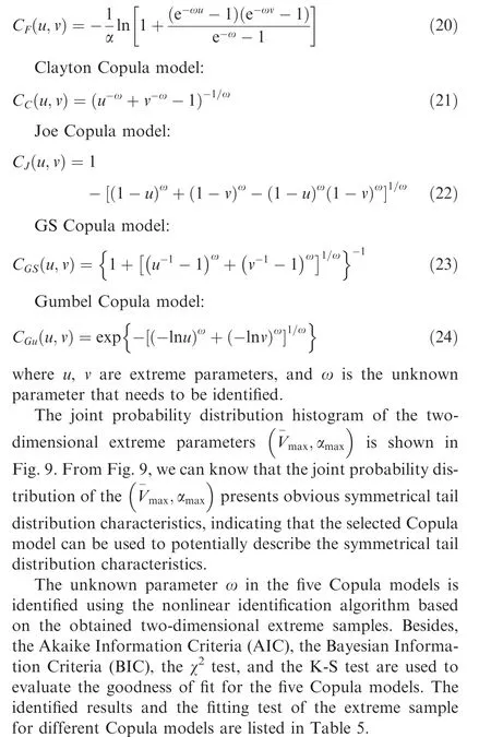
It can be perceived that the P values of the Frank Copula,the Clayton Copula and the GS Copula are all higher than 0.05, indicating that the three Copula models are able to pass the test at the 95%confidence level.The AIC and BIC test values of the Clayton Copula and the GS Copula are smaller than that of other models.It should be noted that the χ2value of the GS Copula is the smallest one among the five models,indicating that its description of the correlation structure of extreme parameters is more accurate than others. Therefore, it can be adopted as a description model of the extreme distribution for two-dimensional extreme samples.

According to the above identification parameter of five Copula models above, to describe the characteristics moreintuitively, the probability density distribution maps are drawn, as shown in Fig. 10. We can see that the probability density map of the GS and the Frank Copula models can better describe the symmetrical tail distribution characteristics of extreme samples.The Clayton Copula model can better reflect the distribution of the lower tail while the Joe and Gumbel Copula models have better ability to describe the upper tail distribution, but the Joe Copula model almost has no ability to describe lower tail distribution.

Table 5 Unknown parameter identification and goodness of fit for five Copula models.

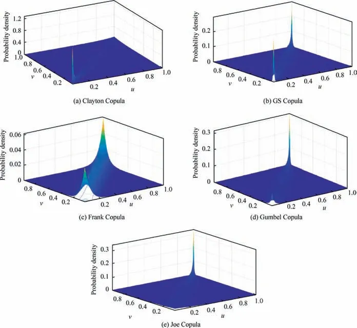
Fig. 10 Probability density distribution maps of different Copula models.

Therefore,based on the definition of flight risk and the GS Copula model, the flight risk probability of two-dimensional extreme parameters can be calculated as

where V-cη( )=Vstable/Vcη( ).

Finally, the flight risk probability in the simulation cases mentioned in the third section is calculated to be 0.1082. It can be found that the value of flight risk probability obtained from the multivariate extreme Copula model is larger than that obtained from the one-dimensional flight parameter GEV model determined by Eqs. (16) and (17). It shows that the flight risk situation that the extreme values of different key flight parameters exceed the limit is fully considered by the multivariate extreme Copula model,and the flight risk is determined more comprehensively and accurately than that of the one-dimensional extreme flight parameters.

4.3. Flight risk probabilities under the effect of different unfavorable factors

The flight risk probabilities in the same initial flight states under the effect of different combinations of unfavorable factors are calculated based on the above methods.The results are listed in Table 6. We can know that the flight risk probability increases with the increase of unfavorable factors,and the risk level is gradually improved.

Since the occurrence of a flight accident is an uncertain process that is dominated by the coupled multi-factor,it is impossible to take all the internal and external unfavorable factors into consideration completely.Therefore,it must be noted that the flight risk probability calculated here is largely a reference value, even though several key disaster-inducing factors have been considered in this study. It is similar to the accident rate in ARP4761 and MIL-STD-882D; however, the calculation methods of flight risk probability in these flight safety specifi-cations are mainly based on the internal hardware failure. In this study,the proposed method can quantitatively assess flight risk,considering not only the failure of the hardware,but also the impact of the external environment. The calculated flight risk probability has a positive significance in the horizontal comparative analysis of flight risk under different conditions and the classification of the risk level.

Table 6 Flight risk probabilities under the effect of different unfavorable factors.

5. Flight safety window under complex conditions

We have discussed the quantitative assessment method of flight risk induced by coupled multi-factor under icing conditions above, while, generally, a deterministic probability of flight risk may not produce a significant meaning. However,visualization of flight risk probability is positive and can enhance the pilot’s situational awareness in complex conditions.This is the main engineering application after the assessment of flight risk. In this study, the flight safety window was used to visualize flight risk.

5.1. Safety window calculation algorithm

The safety window is a color-coded graph that provides information about the risk level of flight parameters or the control surface. The safety window calculation process is shown as follows.

Step 1 Define the window safety palette and break points(a, b, c and d) of each flight parameter x that is related to safety, as shown in Fig. 11, where green is ‘normal’, ξG; light yellow/dark yellow is‘attention’,ξY;light/dark red is‘danger’,ξR; light/deep black is ‘catastrophe’, ξB. x-fis flight state parameter’s lower boundary, and x-fis flight state parameter’s upper boundary.Besides,the points a,b,c and d are set in the light of the actual situation, whose values are determined by the performance of the aircraft and the flight state.

Fig. 11 Risk colors and break points of a safety related flight parameter x.

It is given that where π is the safety palette.

Step 2 The change of each key flight parameter during the forecast time interval can be obtained through flight dynamics simulation of the PAE system as presented in

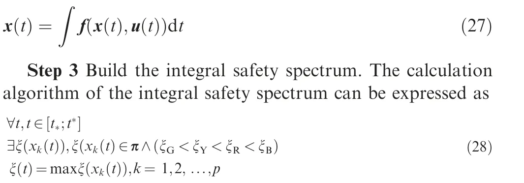
where k is the kth flight parameter; p is the total number of parameters;ξ(t)is the integral safety spectrum color at time t.

From Eq. (28), we can know that the color of risk in the integral safety spectrum is the same with that of the most dangerous risk of all the flight parameters at the same time point.

Step 4 Predict the total flight risk value (R) for the single flight condition. Assume that Pb, Pr, Py, and Pgare the percentage of the four risk colors in the integrated safety spectrum. Vb, Vr, Vy, and Vgare the risk gains for the four colors. R can be denoted as

Here, we give an example to show the safety spectrum for the AOA in a single flight condition and the corresponding integrated safety spectra as shown in Fig. 12.

Step 5 Build the safety window. As discussed in Step 4,the flight risk for a single flight condition is calculated. Then,define the n-factors domain (n=2, 3...), which can be split into several computing units. Each unit corresponds to one single flight situation and the flight risk value of the single flight situation could be obtained by using the method mentioned above. In turn, the risk topological cloud map on the entire computing domain is obtained. The parallel calculation method based on the rapid acceleration mode of MATLAB/Simulink is applied in this study to improve the calculation speed.

5.2. Flight safety window in different situations under icing conditions

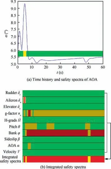
Fig. 12 Integrated safety spectra for a typical flight condition(Vc=150 m/s, θc= 10°, φc= 45°).

According to the calculation algorithm, the flight safety windows in disparate situations are established in this section.The risk division of the parameter for clean (no icing)configuration has been shown in Table 7. Of course, the deterioration of aircraft aerodynamic performance due to ice accretion usually leads to atrophy of the whole flight envelope.Meanwhile, the break points and the boundary will make the appropriate adjustments to what under icing conditions.

In order to illustrate this methodology,the flight safety windows are computed in two cases. The computation was performed on an Intel(R) Xeon (R) (Silver 4110 CPU 2.10 GHz, 32.00 GB RAM).

Case 1. Flight safety window under icing conditions

In order to comprehend whether the pilot’s commands are safe or appropriate under icing conditions, the flight safety windows are needed to calculate. Here, we have built the control system for the aircraft to track the pilot’s commands.Through a designed Proportional-Integral-Derivative (PID)based baseline flight controller, the aircraft can be controlled to track the desired reference values of the velocity (Vc), the pitch angle (θc) and the bank angle (φc).

From Fig. 13, obviously, it is the icing that gives rise to atrophy of the safety operational scope.And the safety operational area grows with the increase of velocity.This is because the aircraft icing increases drag and decreases lift, and as the velocity increases, the kinetic energy goes up, which is able to make up for the energy loss caused by the increased drag so as to maintain stable flight states.As the velocity increases,the safety operational area under icing conditions increases relatively, but it is slower than that under clean configuration.The black regions on the flight safety windows in Fig.13 mark the regions in which the aircraft cannot maintain stable flight states because the expected flight instructions are difficult to achieve, and may cause the aircraft potential loss of control,other than the thought that flight instructions would inevitably cause an accident.

Case 2.Flight safety window in the case of left-side elevator being jammed under icing conditions

The right-side elevator δerand the throttle δthare the main longitudinal control surface when the left-side elevator gets stuck under icing conditions. In order to know the manipulation safety margin of the right-side elevator and the throttle,the flight safety windows are calculated as shown in Fig. 14.

From Fig. 14, we know that, as the icing severity factor increases, the safety manipulation area shrinks bit by bit.The shape of the safe manipulation area under different leftelevator stagnation positions in each case has not varied greatly, and there is just a change in its position in the cloud map.Besides,we can figure out that the safety transitional area is quite tiny,indicating that the pilot must carefully manipulate the stick and the throttle lever to prevent the safety margin from being exceeded.

Table 7 Colored interval of safety related flight data for clean configuration.

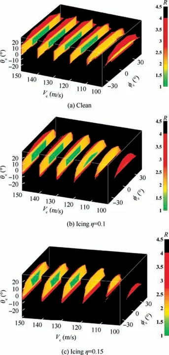
Fig. 13 Flight safety window for a certain aircraft under icing conditions (trimmed at H0=3000 m, V0=120 m/s).

The above proposed method could provide an engineering tool for pilots to manipulate the aircraft safely under complex conditions.The flight risk under different manipulation strategies has been presented to the pilot in an intuitive topological cloud diagram, which will largely enhance the pilot’s situational awareness, and assist in selecting the correct strategy within the safe control range to avoid unsafe manipulation.

5.3.Application of flight safety window in designed icing warning system

How to combine ergonomics with the above icing safety measures to provide the intuitive warning and guidance to pilots,is a universal subject with important research value.From the literature published at home and abroad, there are rare researches on the icing warning and manipulation guidelines in Head-Up Display(HUD).In view of the unique advantages of HUD,it is of great significance to study how to construct an icing indication and warning system based on HUD.

In this study,the icing indication and warning system based on HUD have been constructed as shown in Fig.15,and especially Fig.15(a)shows the icing indication interface on HUD.In addition to the normal display function,the over-limit indications of the AOA, roll angle and flight speed are added on the HUD, and Fig. 15 (b) presents the icing warning system interface.The icing warning messages cover:the icing position and severity,and the working status of the icing envelope protection system and the deicing system.A flap limit message will appear when the flaps deflection is beyond safe limits.And the color-coded control surface icing condition indicators are used to show the icing severity and the icing position. The control surfaces color will change according to the icing severity.With no icing, the control surfaces color is green. When there is a caution displayed for the medium icing, the surfaces turn yellow.When there is a warning displayed for the severe icing,the surfaces will turn red.

The integral flight safety spectrum of six critical safety parameters is presented in the interface to remind the pilots which parameters will be overrun and then how to avoid dangerous situations with proper manipulation.

The icing indication and warning system can be realized by Mix Reality (MR) technology. The hardware structure diagram of the system is shown in Fig.16.The designed interfaces of the icing indication and warning system shown in Fig. 16 can be superimposed on the pilot’s line of sight through Holo-Lens mixed reality glasses.

The system can effectively enhance the pilot’s infiltrating experience,achieve indication and warning in icing encounters,and improve the flight safety under icing conditions. The system can be used in icing flight simulation training for pilots to experience the unfavorable maneuvers that may cause the aircraft loss of control under icing conditions.

6. Conclusions

In summary, novel methodologies for quantitative assessment and visualization window of flight risk under icing conditions have been proposed in this study.

(1) By using Monte-Carlo simulation and multivariate extreme value theory, we have emphatically proposed a method to quantitatively assess the flight risk induced by multi-factor coupling under icing conditions. The randomness and uncertainty of multiple factors (the single-sided elevator jamming and AOA sensor fault)that may happen in the PAE system in icing encounters are considered in the modeling process. Through thousands of times of Monte-Carlo simulation on the realtime flight simulation platform, the extreme samples of two parameters (Vmin, αmax) are extracted and proved to present the GEV distribution characteristics.Besides,the correlation structure of the two-dimensional extreme parameters has been analyzed based on Copula theory,and it is shown that the GS Copula model can most accurately describe the joint distribution of twodimensional extreme parameters through goodness of fit tests.And the flight risk probabilities under the effect of different adverse factors obtained from the multivariate Copula model prove that the flight risk probability increases with the rise of unfavorable factors.The quantitative assessment method proposed in this study could be an effective supplement to flight risk assessment methods in the existing flight safety specifications such as SAE ARP-4761.

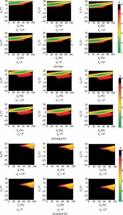
Fig. 14 Flight safety window in the case of left-side elevator being jammed under icing conditions (trimmed at H0=3000 m,V0=120 m/s).

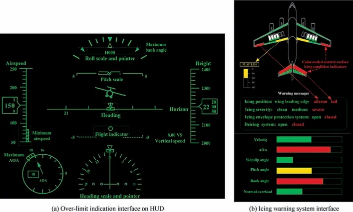
Fig. 15 Icing indication and warning system interfaces.

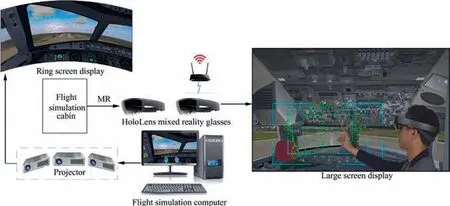
Fig. 16 Hardware structure of icing indication and warning system.

(2) Besides, a flight risk visualization method named flight safety window proposed in this paper is a qualitative tool using a color-coded graph instead of a hard-line value to denote safety related parameters. The flight safety window visualization of predicted evolution of the various flight parameters nicely illustrates what happens under the analyzed conditions. The obtained safety window gives the safe manipulation envelope of the key parameters and flight instructions from the colorization of flight risk probability. The flight safety window could be a nice teaching tool as it clearly illustrates the relationship between flight parameters and unsafe states, and processes the potential application in the designed icing indication and warning system for the pilot to keep the aircraft in the safe region under icing conditions.

This paper mainly focuses on the flight safety in longitudinal direction which is the paramount under icing conditions.In future studies,the flight safety in multi-axis coupling situation will be fully considered under icing conditions.

Acknowledgement

This study was supported by the National Key Basic Research Program of China (No. 2015CB755802).