A new online modelling method for aircraft engine state space model

Shuwei PANG, Qiuhong LI, Haibo ZHANG

Jiangsu Province Key Laboratory of Aerospace Power System, Nanjing University of Aeronautics and Astronautics,Nanjing 210016, China

KEYWORDS Aircraft engines;Component level model;Online modelling;Partial derivative;State space models

Abstract To overcome the drawbacks of current modelling method for aircraft engine state space model,a new method is introduced.The form of state space model is derived by using Talyor series to expand the nonlinear model that is implicit equations and involves many iterations. A partial derivative calculation method for iterations is developed to handle the influence of iterations on parameters. The derivative calculation and the aerothermodynamics calculations are combined in the component level model with fixed number Newton-Raphson (N-R) iterations. Mathematical derivation and simulations show the convergence ability of proposed method. Simulations show that comparing with the linear parameter varying model and centered difference based state space model,much higher accuracy of proposed online modelling method is achieved.The accuracy of the state space model built by proposed method can be maintained when the step amplitudes of inputs are within 2%,and the responses of the state space model can match those of the component level model when each input steps larger amplitudes.In addition,an online verification was carried out to show the capability of modelling at any operating point and that state space model can predict future outputs accurately. Thus, the effectiveness of the proposed method is demonstrated.

1. Introduction

Aircraft engine mathematical model has great potential in control and simulation.1-3Many researches about aircraft engine modelling methods have been published, and Component Level Models (CLMs), State Space Models (SSMs) and artificial intelligent networks are the most typical models.

CLMs can operate in a wide flight envelope and complete different simulations for different purposes.4-9Many improvements for CLMs are proposed, such as utilizing a Neuro-Fuzzy model to predict component performance parameters,10,11solving the model with new methods12,13and so on.Though these improvements simplify the calculations of the CLM and reduce the computation load, CLM’s calculations are still complex and time-consuming. In contrast, the SSM14-16and the intelligent network17-20have lower computation burden, and these simplified models are more viable as onboard models in terms of real-time property, especially for online model based applications, such as Model Predictive Control(MPC),Extended Kalman Filter(EKF)based performance estimation and performance seeking control, in which the model has to be called repeatedly to get the optimal solution.In addition,the SSM is widely used in controller design in the framework of linear system theory.21-24

So far, two major modelling methods for SSM have been developed, namely fitting method,25,26and difference based partial derivative method.27-31The fitting method uses system identification theory and optimization approach to get the parameters of the model. The partial derivative method uses the Talyor series expansion approach and Jacobian matrix calculation to get system matrices from the nonlinear model directly. But the partial derivative has to be calculated by difference methods in practice because there are some complicated operations such as interpolations and iterations, in the nonlinear CLM of aircraft engine.

However, these two methods have some disadvantages. In terms of real-time property,the fitting method needs to collect response data and model a SSM by fitting the data offline.For the partial derivative method, the CLM needs to be called repeatedly because of difference methods, and the frequency of calling the CLM increases as the number of independent variables of the SSM goes up,which limits the speed of acquiring a SSM. It means that these two methods cannot be implemented online to generate accurate SSMs for every operating point due to poor real-time property.In addition,all the independent variables except a perturbed variables have to be kept unchanged in iterations when difference methods are utilized,which is actually hard to be realized. Thus, this method may be not suitable for calculating the system matrices of health parameters in the Kalman filter directly because the health parameters degrade together in an aircraft engine, which proposes a demand for obtaining partial derivatives with all the health parameters being perturbed simultaneously.27

Secondly, only finite operating points can be modelled offline by these two methods due to aero-engine’s strong nonlinearity and wide operation envelope. SSMs of other operating points only can be obtained by interpolation or parameter scheduling method like Linear Parameter Varying (LPV)method and so on.15,27,32-38The acquired SSMs are less accurate than models built directly at the same operating point.These offline modelling techniques may be enough for the design of controllers such as H∞and linear quadratic regulator but not in the case that the model is required to be available at every operating point in applications like MPC and EKF.

In the design of Kalman filters,the SSM is used to estimate performance and sensor outputs in health monitor and fault diagnosis39-45and also to estimate unmeasurable parameters such as thrust and surge margin indirectly.46-48However, system matrices of SSMs are required to be updated for estimations in the recursive process when Kalman filters are chosen, especially EKF and Linearized Kalman Filter(LKF).49-51Furthermore, estimation errors will exist if the accuracy of the model at current operating point cannot be guaranteed,which proposes a demand for continuous updates of the model.

In addition, the SSM can be used as a predictive model in MPC’s control architecture.16,52-54The benefit of MPC is that future outputs can be predicted properly by onboard models,which can help control system to optimize input sequence to make the performance indices of the whole system reach the optimum. But the advantage may be destroyed if the model is obtained from piece-wise linear models or parameter scheduling techniques because of the model precision and uncertainties of engine.

In this paper, a new online modelling method for aircraft engine state space model is proposed to keep pace with above demands. A general nonlinear model that actually is implicit equations is expanded to a discrete state space model firstly.Then, a partial derivative calculation method for iterations is developed to handle the complex iterations of CLM. Finally an online modelling method that combines a CLM and a partial derivative calculation with fixed number Newton-Raphson(N-R) iterations is presented. It can build the SSM for any operating point, and there is a SSM generated every sample period,which shows the online modelling capability of the proposed method.Thus,the accuracy of SSMs can be guaranteed in the flight envelop.Besides that,the system matrices of SSMs can be highly accurate because the operations such as parameter perturbations and finite difference calculation are dismissed, and these matrices are derived analytically by the partial derivative calculation method that involves differential calculation rather than typical derivation method or difference method.

The paper is organized as follow. Section 2 introduces the form of SSM derived from the CLM.Section 3 present a basic calculation principle. Section 4 proposes the online modelling method that involves multi-iterations and shows its convergence analysis. Section 5 implements proposed modelling method in the CLM. Section 6 shows and discusses the simulations and Section 7 concludes this paper.

2. State space model derived from CLM The SSM is built based on the CLM.Without loss of generality, suppose that a trajectory of engine operating point in a period of time is shown as Fig. 1, and the horizontal axis is time and the vertical axis is engine state. This trajectory can be achieved by a typical acceleration process.

The parameters of state space models vary with the engine operating state because of the strong nonlinearity and variable parameter characteristics of the aero-engine,which means that the state space model established has parameter-varying characteristics during transient operation.

The nonlinear state space model of a typical CLM of twinspool aero-engine can be described as

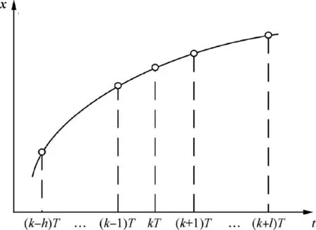
Fig. 1 Sketch of engine operating point trajectories.

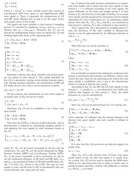
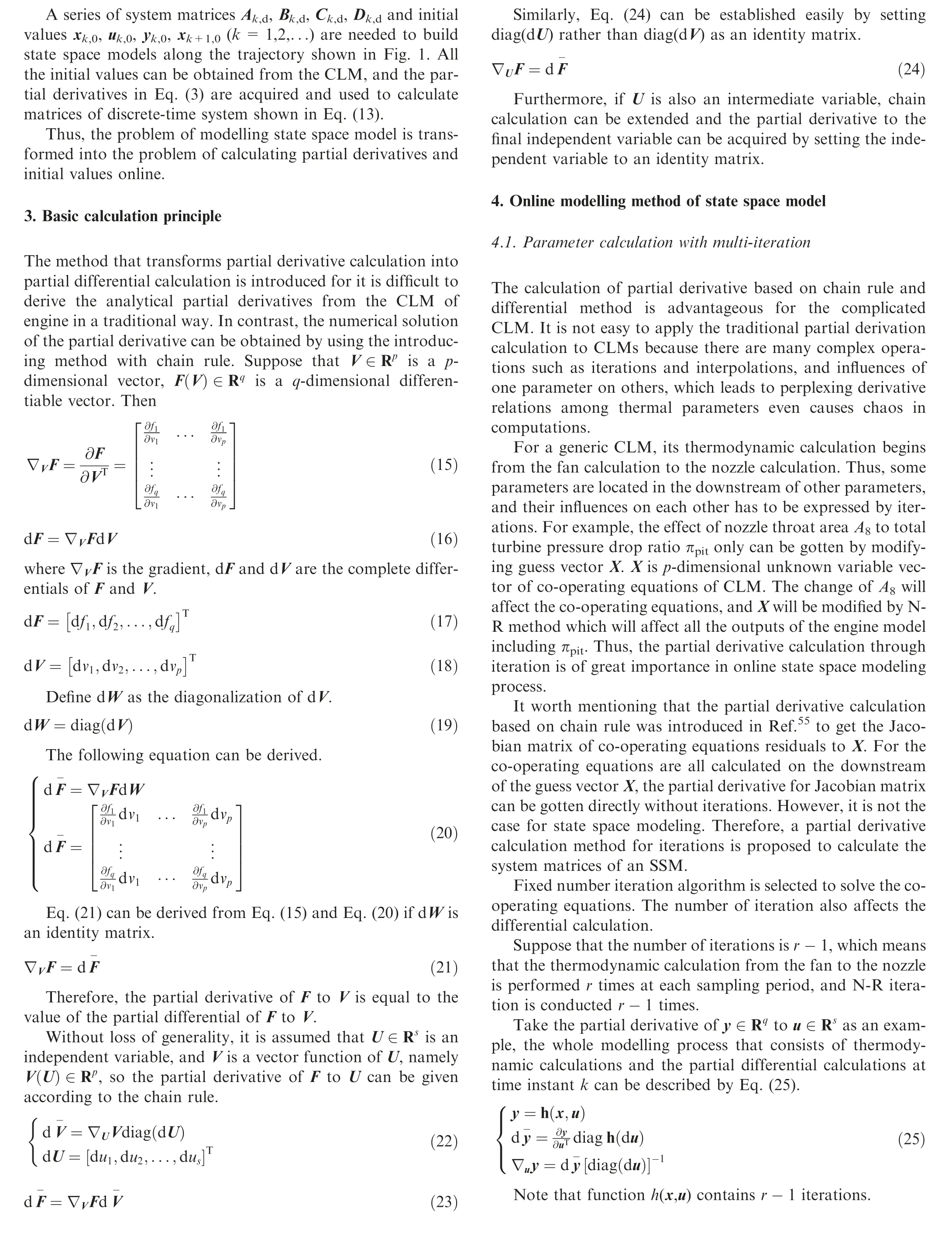
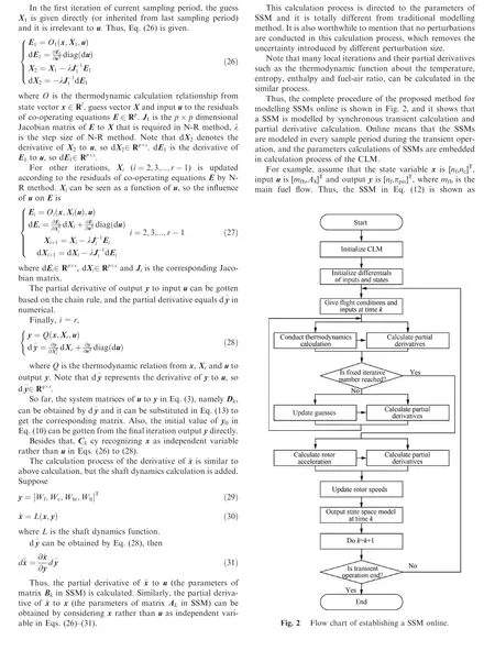
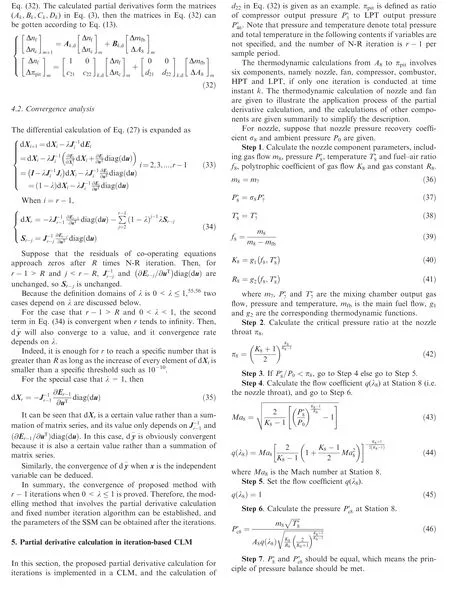
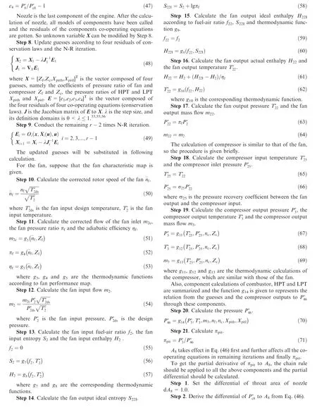
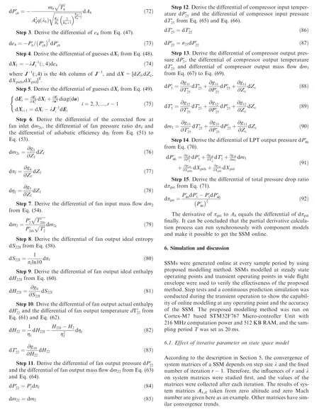
Fig.3 shows the changes of elements of Ak,dobtained at the steady state point as the step size λ and the number of iterations vary.The horizontal axis denotes iterative number,the vertical axis represents the value of each element of Ak,d.For example,a11is the first element of the first column in Ak,d,a12is the first element of the second column in Ak,d,and so forth.

Fig. 3 shows that different matrix elements are obtained with different iterative numbers when the step size λ is unchanged, and the same element with different λ converges to a same value. The convergence speed of the elements is influenced by λ,and a larger step size can lead to a faster convergence speed. About 60 iterations are required to make the elements converge if the step size λ is set as 0.1 whereas only one iteration is enough if the step size is 1.0.

The simulation of the transient operating point was conducted by same method, and Fig. 4 depicts the convergence curve of Ak,dfor the transient operating point.

The number of iterations and step size have the same effect on elements’convergence as that at the steady point.When λ is set as 1.0,the elements reach convergence after two iterations.But it should be mentioned that the changes of elements after one iteration are very small, and the element values has approximated the final convergence values.

For the cases that step size λ is 0.1 and 0.5,all the elements in Figs.3 and 4 converge approximate exponentially both at a steady state point and at a transient point. This is because the co-operating equations have been convergent after R times NR iterations, only the term (1-λ)j-1in Eq. (34) continues to decrease at exponential convergence rate, which results in the convergences of the elements. In addition, the decay rate of the term(1-λ)j-1depends on λ when 0<(1-λ)<1,and less iterative number is required in the case λ=0.5 than the number in the case λ=0.1 because the decay rate is greater when λ=0.5. Note that every term in Eq. (34) changes before the co-operating equations become convergent,so the convergence rate is not exponential at the beginning of the iteration. However, the influence of this process on the convergence rate of elements can be ignored because the co-operating equations become convergent quickly due to N-R algorithm’s superlinear convergence rate,56which means that this process only appears in initial iterations.

For the case λ=1,Figs.3 and 4 show that the convergence of elements at a steady point and at a transient point is slightly different. Only one iteration is required to get convergent and accurate elements for a steady state point while more than one iteration are needed for a transient point. The reason is that the co-operating equations have been convergent for a steady state point,so every term in Eq.(35)is unchanged.In contrast,several N-R iterations are required to make the co-operating equations convergent first for a transient operating point.Indeed, the initial value of unknown variable X comes from the solution of last period, so it will not deviate far from current solution in a continuous simulation process,so X can converge quickly after a small number of N-R iterations with large λ.Thus,it can be seen that the elements converge sharply when λ=1.

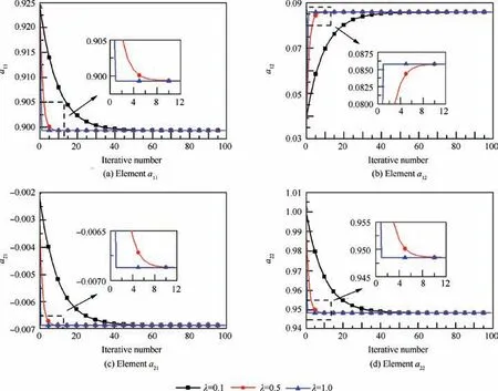
Fig. 3 Changes of elements with iterative numbers and step sizes at steady state point.

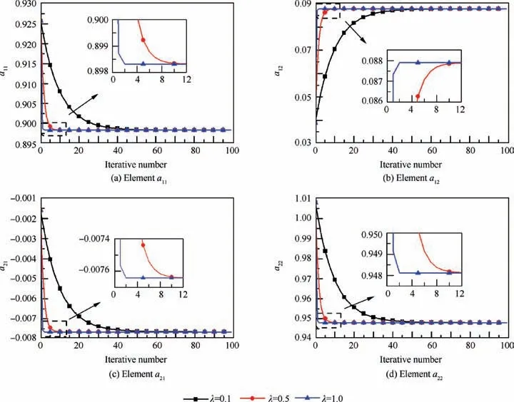
Fig. 4 Changes of elements with iterative numbers and step sizes at transient point.

Above results and discussion demonstrate the convergence of proposed method,which matches the deduction in Section 5 well. Also, for ensuring convergence, the proper parameter combination λ=1 and r=5 is implemented in the following experiments.

6.2. Simulation of modelling in steady state

6.2.1. Simulation at ground

Step simulations were conducted to show the accuracy of proposed Online Modelling Method based SSM (OMMSSM),and step responses at zero altitude and zero Mach number were presented when each input stepped different size. The main fuel flow mfbwas 0.99 kg/s and A8was 0.28 m2.

The responses of OMMSSM was compared with responses of the CLM,a LPV model and a Centered Difference Method based SSM (CDMSSM). The LPV model was built according to the method described in Refs.27,28, and the CDMSSM was established by centered difference method based Jacobian linearization with 1% perturbation size.57

Figs. 5 and 6 present the responses when mfband A8step 2% respectively. Note that all the variables were normalized by using the design point values, so the percentage changes of same variables can be compared easily.

Figs.5 and 6 show that the responses of the OMMSSM are basically the same as that of the CLM. In particular, the response of πpitof the CLM has a relatively sharp overshoot when A8steps, and the outputs of the OMMSSM can match these increases effectively. In contrast, the responses of the LPV model and the CDMSSM deviate from the responses of the CLM significantly and converge to different values.

Table 1 is given to describe steady state relative errors of the model responses comparing with CLM’s responses when mfband A8stepped respectively. This table clarifies the applicable range and accuracy of the OMMSSM,the LPV model and the CDMSSM.Note that all the value listed in tables are absolute values and the relative error of terminal value is defined as follow.

where ΔySSMand ΔyCLMare the terminal values of step response of the SSM and the CLM respectively.Note that they are increments relative to the values of the operating point where the SSM built.

Because the SSM is a linear system,its response magnitude is proportional to the input magnitude.So is the LPV model at a certain operating point. But the CLM is nonlinear, so its response magnitude is not proportional to the input magnitude. Therefore, the steady state relative errors vary with the input magnitude. Table 1 shows that the OMMSSM has a higher accuracy than the LPV model and the CDMSSM,and its errors vary from 0.0465% to 3.2897%. In contrast,most errors of the LPV model and the CDMSSM are much larger than that of the OMMSSM, which reach up to 6.3082% and 12.5886% respectively. In addition, for the OMMSSM, the steady state relative errors are smaller than 2% when the amplitude of mfbis within 3%. In contrast, the steady state relative errors can be kept smaller than 1% when the amplitude of A8is within 3%.

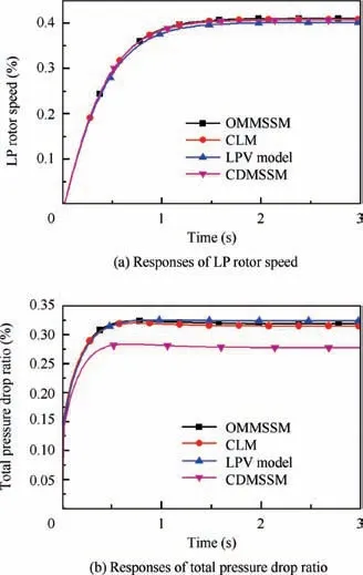
Fig. 5 Response comparison when mfb stepped 2% at steady state point.

6.2.2. Simulations in flight envelope

Step simulations at other steady state points in flight envelope were conducted, and the simulation conditions are listed in Table 2. The responses of the OMMSSM, the LPV model and the CDMSSM were also compared with that of CLM when mfband A8stepped respectively,and steady state relative errors are shown in Table 3.

Table 3 shows that the responses of the OMMSSM built at other steady state points in flight envelope are in line with the responses of the CLM.When the step amplitude is within 2%,the maximum relative errors of nfand πpitof the OMMSSM are 2.2963% and 1.0545% respectively. Moreover, Tables 1 and 3 show that the relative errors of the OMMSSM are smaller than 1% for most cases. However, the errors of the LPV model rise to 19.3834% and 21.7040% with the 2% input steps. The errors of πpitresponses of the CDMSSM also increase to a high level, of 10.7405%. The results show not only the superiority of online modeling method to the LPV modeling method in model accuracy over the envelop but also the great benefit of exact derivative calculation than the central difference calculation in model accuracy over the envelope.

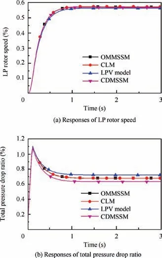
Fig. 6 Response comparison when A8 stepped 2% at steady state point.

Overall, the responses under small perturbations of the inputs can be modelled appropriately by proposed online modelling method,and the OMMSSM has a much higher accuracy than the LPV model and the CDMSSM. The simulations also demonstrate that the proposed method can be applied to the SSM modelling of steady state points, and high accuracy can be maintained when inputs make a step within 2% amplitude,which indicates the modelling ability of proposed method.

6.3. Simulation of modelling in transient state

6.3.1. Simulation at ground

In the ground transient simulation, the main fuel flow increased from 0.99 kg/s to 1.2 kg/s at 0.02 kg/s per sampling period, and the SSM at the operating point of which mfbwas 1.09 kg/s was taken as an example to show the result of step test.

Figs. 7 and 8 show the responses when mfband A8stepped 2%respectively.Note that all the variables are also normalized by using the design point values.

Figs.7 and 8 show that the responses of the OMMSSM can match that of the CLM properly when each input steps 2%.However, there are significant differences between the LPV model and the CLM’s outputs for transient responses and terminal values, and the transient responses of πpitof the CDMSSM is also different from the CLM’s although its terminal values are close to the CLM’s.

Table 4 lists steady state relative errors when the step amplitude of each input varies from 1% to 5%. Table 4 shows that the responses of the OMMSSM built during the transient operation are consistent with that of the CLM when the step amplitudes are smaller or equal to 2%,and the steady state relative errors can remain in the range of 2%.Besides that,all the errors are smaller than 4% even step amplitudes increase to5%, which indicates that the OMMSSM can provide a good estimate of outputs at the transient operating point. In contrast, the errors of the LPV model and the CDMSSM can reach up to 68.6165% and 12.1991%, which are much higher than the maximum error of OMMSSM.

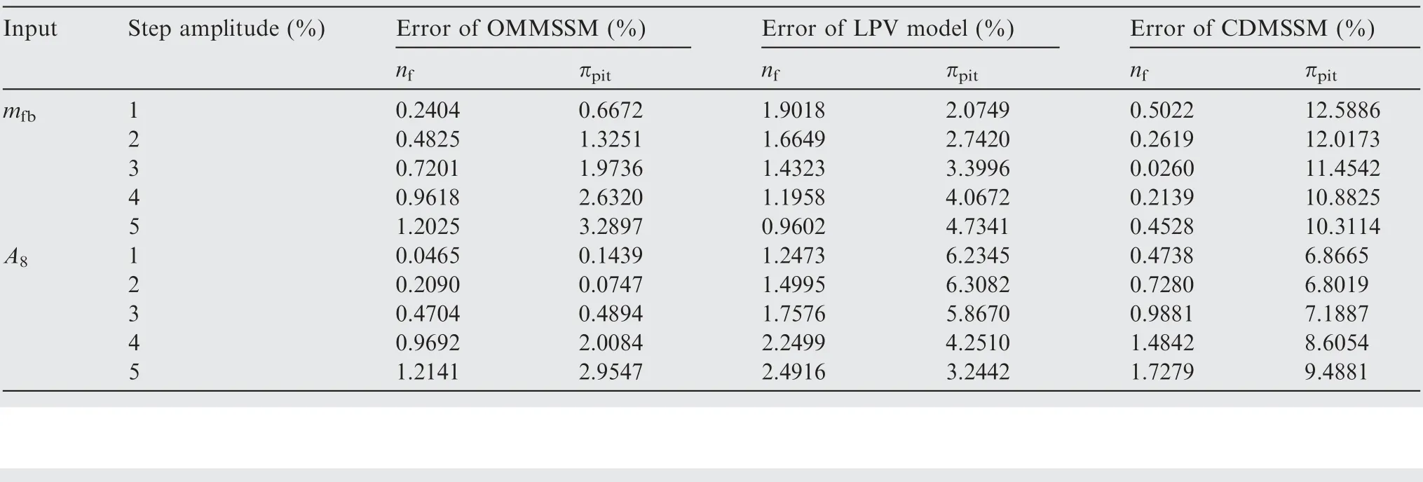
Table 1 Relative errors of terminal value of SSM built at steady state when inputs stepped.

Table 2 Simulation conditions for steady state points.

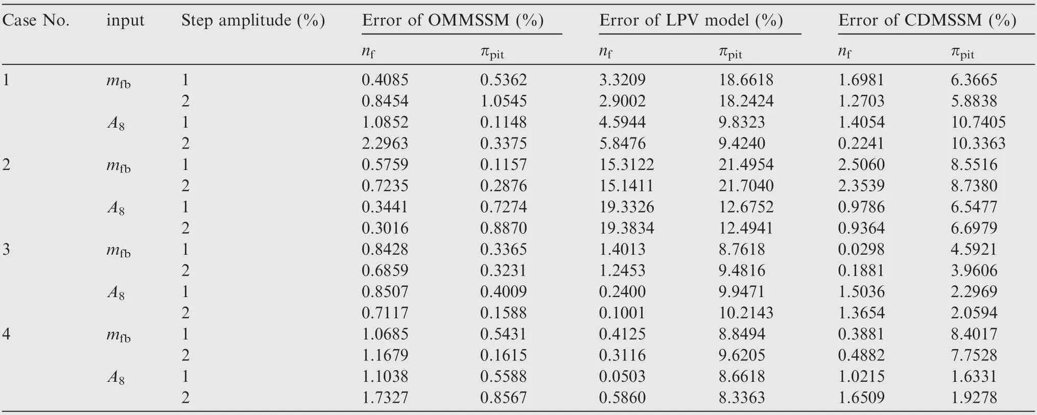
Table 3 Relative errors of terminal value of SSM built at steady state in flight envelope when inputs stepped.

6.3.2. Simulations in flight envelope

In order to further verify the modelling method for transient operating points, transient simulations within flight envelope were conducted, and the flight conditions and inputs are shown in Table 5.

The transient operation was simulated by initializing the model at condition Case 1 and then changing the flight conditions and inputs of one point to that of next point in turn.The change rates of altitude, Mach number, mfband A8per sampling period are 0.02 km, 0.01, 0.02 kg/s and 0.001 m2respectively.

The transient verification operation points are shown in Fig. 9 by normalized nfand πpit, and the SSMs of four transient operating points denoted by Points 1,2,3 and 4 from left to right in Fig.9 were taken as examples to verify the accuracy of the SSMs. The relative errors of steady terminal value of step responses are given in Table 6.

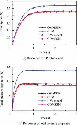
Fig. 7 Response comparison when mfb stepped 2% at transient operating point.

Table 6 shows that the responses of the OMMSSM built during the transient operation can match that of CLM, and errors are less than 3% except the error when A8step 2% at Point 3. It indicates that the SSM built by proposed method can maintain a high accuracy at transient operating points in the envelope when the amplitudes of perturbations are smaller than 2%. Besides that, the errors of nfand πpitof the OMMSSM vary from 0.0206% to 3.2222% and from 0.0568% to 2.9789% respectively. In contrast, the errors of the LPV model change from 0.7340% to 46.8153% for nfand from 1.8318% to 52.4449% for πpit, and the errors of the CDMSSM change from 0.0264% to 17.9798% for nfand from 0.0615% to 41.1476% for πpit. Therefore, the errors of the OMMSSM are smaller than those of the LPV model and the CDMSSM, which indicates that the OMMSSM can estimate the transition property more accurately than the LPV model and CDMSSM.

By comparing the results of model built at steady state points with that of transient operating points, it can be found that the overall relative errors of terminal value of the OMMSSM built at transient operating points are greater than those at the steady state points, which is due to the more changeable transient characteristic of engine. For the SSMs of steady state points, their average relative errors are 0.60%and 0.78% respectively when the input steps 1% and 2%respectively according to Table 3 whereas the average relative errors for SSMs of transient points are 1.12% and 1.31%respectively according to Table 6.

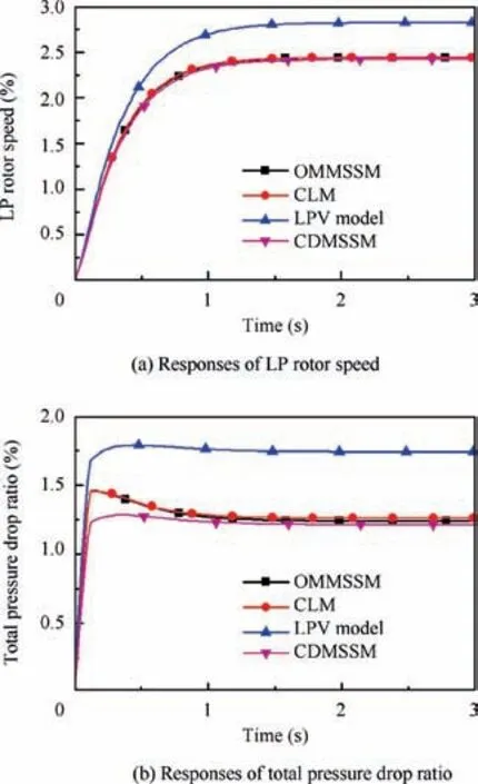
Fig. 8 Response comparison when A8 stepped 2% at transient operating point.

Overall,the simulations at steady state and during transient operation both show that the proposed modelling method can establish a more accurate SSM than LPV method and center difference based method. This advantage mainly depends on accurate derivative calculation.In proposed method,the Jacobian matrices are calculated analytically and numerically online, so the parameters gotten from derivative calculation can reflect the characteristic of engine accurately, which make the OMMSSM achieve a high accuracy for its modelling principle.On the contrary,centered difference method is numerical calculation method,and it is an approximate algorithm in nature. One percent perturbation size may not be the best option for all the operating points. CDMSSM may achieve the same accuracy after the perturbation size is fine-tuned, but it is impossible and difficult to tune the perturbation size for every operating points.The accuracy of LPV model is limited due to the fact that it is a fitting model of finite SSMs essentially,so its accuracy will drop when it is applied to unmodeled points in the envelope. Thus, the proposed modelling method is more capable and benefit for modelling the SSM in wide flight envelope.

Besides that,it is worthwhile to mention that the time consumption for building an OMMSSM is 12.8040±0.1755 ms while the time consumption for building a CDMSSM is 76.6101±1.0906 ms. This results show that the proposed method requires much less time to build a SSM than center difference based method, For a control system with sample period 20 ms, the SSM can be gotten online in real-time.Furthermore, proposed modelling method generates a SSM at every sample period, so modelling capability of proposed method is demonstrated.

Table 4 Relative errors of terminal value of SSM built at transient operating point when inputs stepped.

Table 5 Simulation conditions for transient points.

6.3.3. Prediction simulation in flight envelope

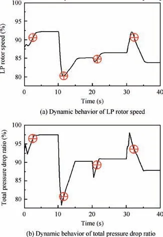
Fig. 9 Transient operation simulation under condition listed in Table 5.

An online simulation was performed to demonstrate the capability of online modelling and verify the accuracy of the SSM for prediction purpose. The transient operation shown in Fig. 9 was performed, and SSMs were gotten at every time instant k. It was used to predict future outputs from time instant k+1 to k+5 online with the same flight conditions and inputs as that of the CLM. The predictions at k+1, k+3 and k+5 are compared with the outputs of the CLM at the same time instant.

Figs.10 and 11 represent the comparison of the predictions of nfand πpitat time instant k+1. Figs. 12 and 13 show the comparison of the predictions at time instant k+3, and Figs. 14 and 15 give the comparison of the prediction at time instant k+5. All the predictions were gotten by the response of SSM obtained at time instant k,and the SSM were updated with the receding horizon. Note the variables are normalized.

It can be seen from Fig.10 to Fig.15 that the SSMs built by proposed method can predict future outputs efficiently, and the maximum errors of nfand πpitare within 0.5% and 2%respectively. Concretely, the maximum prediction error for LP rotor speed nfis about 0.4% when the SSM built at time instant k is used to predict the nfat time instant k+1,and this maximum prediction error witness a ignorable increase, from 0.4%to 0.45% when the SSM it used to predict the nfat time instant k+5. The prediction error of πpitalso increase slightly, from about 0.4% to 2% when receding horizon increases from k+1 to k+5. It is worthwhile to mention that although the errors of πpitincrease more than that of nfdoes, the prediction accuracy is still very high.

Thus, these results indicate that the accuracy of the predictions can be guaranteed by the SSM built. This is mainly because the exact derivative calculation is adopted and the SSM can be updated every sample period.It also suggests that proposed online modelling method is effective and can be used to provide accurate onboard model for some applications such as EKF and MPC.

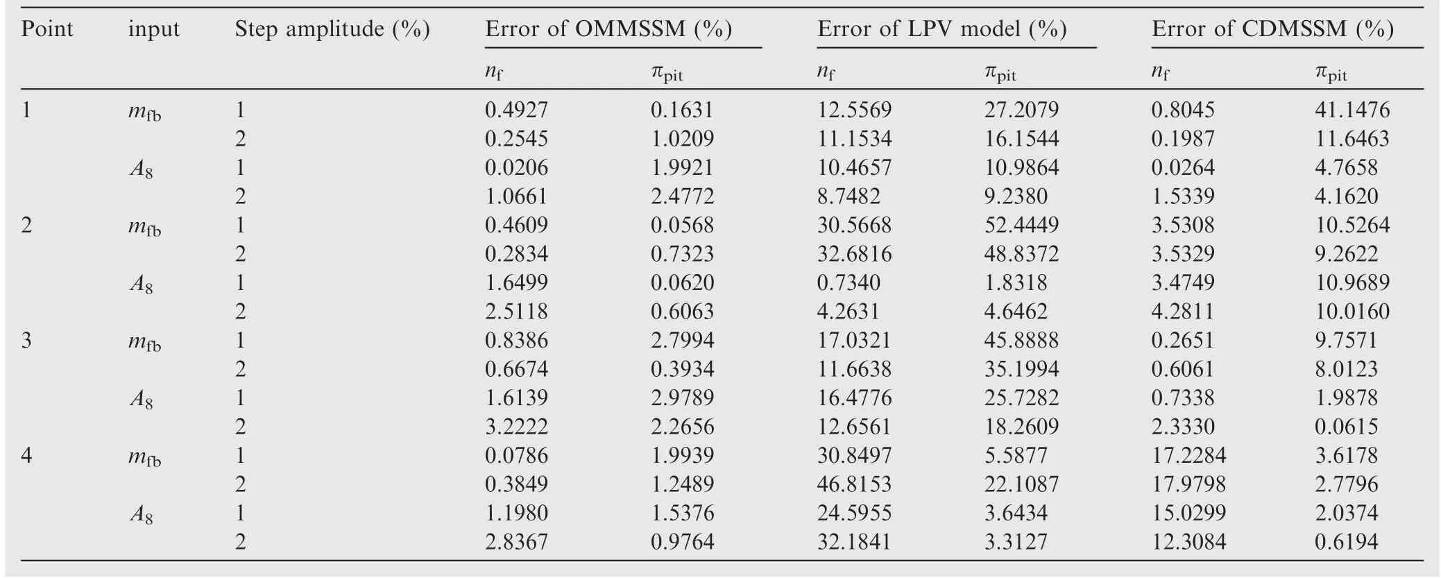
Table 6 Relative errors of terminal value of SSM built during transient operation in flight envelope when inputs stepped.

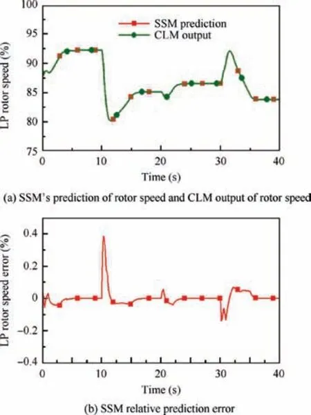
Fig. 10 LP rotor speed change and prediction error at time instant k+1.

Besides that, note that the prediction errors can be zero when the engine is at steady state. At steady state, the input of SSM Δuk，m=0, the state of SSM Δxk，0=0, so the output Δyk，m=0, so yk，m=yk，0, and yk,0is taken from CLM, which leads to the prediction of SSM is equal to yk,0.

Overall, the above simulations demonstrate the effectiveness of proposed method for online modelling at steady state points and transient operating points in wide flight envelope.

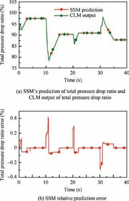
Fig.11 Total pressure drop ratio change and prediction error at time instant k+1.

7. Conclusions

(1) An online modelling method for aero-engine state space model is proposed, and it takes advantage of a CLM and a partial derivative calculation for iterations to get accurate SSMs.The proposed partial derivative calculation method for iterations is capable for calculating exact derivatives of complicated system involving iterations,and there is no demands for conducting perturbations. The form of SSM deduced by Talyor series expansion can describe the models at steady state points and transient operating points.

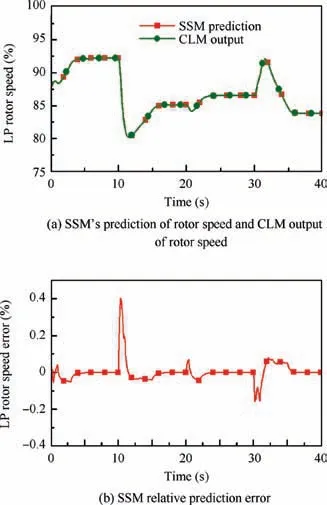
Fig. 12 LP rotor speed change and prediction error at time instant k+3.

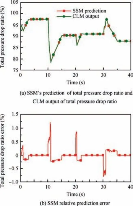
Fig.13 Total pressure drop ratio change and prediction error at time instant k+3.

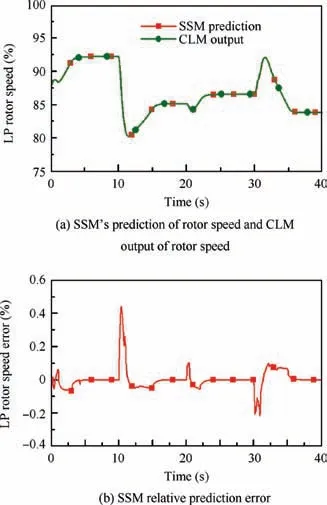
Fig. 14 LP rotor speed change and prediction error at time instant k+5.

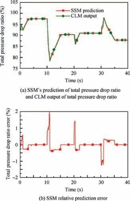
Fig.15 Total pressure drop ratio change and prediction error at time instant k+5.

(2) The convergence of proposed method is proved by mathematical deduction and convergence simulations,and the number of iteration and step size of N-R method affect the final parameters of the SSM.

(3) The validation simulations were carried out at steady state points and transient operating points in wide flight envelope. Results show that the responses of the OMMSSM can match that of the CLM precisely at the corresponding operating point when inputs step 2% or less, and high accuracy of established models can be guaranteed. Moreover, the SSM can reflect the changes of outputs properly under the condition of larger perturbations of inputs.By comparing with the LPV model and the CDMSSM, simulations show that the OMMSSM has a higher accuracy that benefits from continuous updates of the system matrices and accurate derivative calculation.Besides that,the time consumption of building an OMMSSM is only about 13 ms, which can meet the real-time requirement (20 ms every sample period).

(4) A prediction simulation was conducted online in wide flight envelope to verify the capability of modelling at any operating point and the accuracy of SSM for some prediction applications. The results show that the OMMSSM built online every sample period can be used to predict parameters over next several steps accurately.Thus, the online modelling capability and effectiveness of presented method is further demonstrated.

(5) There are many potential applications where the proposed method can be applied. For example, it would be interesting to explore how to provide MPC controller with an optimization-oriented adaptive model in realtime in our future work. With proposed modelling method, the model not only can predict parameters accurately but also lower the computation burden. For another example, a huge amount of SSM can be gotten easily for various operating conditions by proposed online modelling method,which can be helpful for other researches of engine,such as cluster analysis and feature extraction.

Acknowledgement

This study was supported by the Postgraduate Research &Practice Innovation Program of Jiangsu Province, China(No. KYCX18_0315).