A novel variable structure multi-model approach based on error-ambiguity decomposition

Hn SHEN-TU, Yingjio RONG, Dongling PENG, Mengfn XUE,Yunfei GUO

a Institution of Information and Control, Hangzhou Dianzi University, Hangzhou 310018, China

b Science and Technology on Near-Surface Detection Laboratory, Wuxi 214035, China

KEYWORDS Error-ambiguity decomposition;Maneuvering target tracking;Model sequence set adaptation;Multi-model estimation;Variable structure

Abstract Model Set Adaptation (MSA) plays a key role in the Variable Structure Multi-Model tracking approach (VSMM). In this paper, the Error-Ambiguity Decomposition (EAD) principle is adopted to derive the EAD-MSA criterion that is optimal in the sense of minimizing the square error between the estimate and the truth. Consequently, the EAD Variable Structure first-order General Pseudo Bayesian (EAD-VSGPB1) algorithm and the EAD Variable Structure Interacting Multiple Model (EAD-VSIMM) algorithm are constructed. The proposed algorithms are tested in two groups of maneuvering target tracking scenarios under different modes and observation error conditions.The simulation results demonstrate the effectiveness of the EAD-VSMM approach and show that, compared to some existing multi-model algorithms, the proposed EAD-VSMM algorithms achieve more robust and accurate tracking results.

1. Introduction

Single model Bayesian target tracking algorithms are applied well to the non-maneuvering target tracking problems. However, the single model algorithms are not suitable for the maneuvering target tracking problems for the target performs different maneuvers at different time stamps, and these random maneuvering modes are usually unknown to the tracking algorithms. Although we can use a single model Bayesian tracking algorithm to track the maneuvering target,a tracking failure may occur when there is a mismatch between the prior motion model and the real maneuvering mode.1

To solve the above mentioned problem, the multi-model approaches arose and the maneuvering motions are described by hybrid systems with discrete modes and continuous states.2,3The key idea of the multi-model approach is that if it is difficult to describe the maneuvers by one model, one can use a set of models to cover all possible maneuvering modes. As the consequence, the target real mode is approximated by the combination of multiple models with suitable weights. Therefore, for the multi-model tracking approaches,the tracking quality depends on the quality of the model set as well as the estimated model weights.4

Generally, it is difficult to fulfill the optimal multi-model algorithm. On the one hand, the optimal multi-model algorithm should be constructed based on the optimal model sequence set. However, it is not trivial to obtain the optimal model sequence set in general. On the other hand, even if the optimal model sequence set is available, we still need to consider the full hypothesis tree for the optimal multi-model algorithm. Thus, many suboptimal approaches were proposed in last decades, include the Static Multi-Model (SMM)approaches,5the General Pseudo Bayesian (GPB)approaches,1,6the Interacting Multi-Model (IMM)approaches,7-9as well as the Variable Structure Multi-Model(VSMM) approaches.10,11As the simplest multi-model algorithm,the SMM uses a fixed model set to cover the real modes and is suitable for some weak maneuver scenes. However, the results of the SMM may deteriorate when the target undergoes frequent mode changes. For the maneuvering targets with frequent mode changes, the GPB and IMM algorithms are more suitable than the SMM algorithms for they describe the mode changes by the Markov chains. Then, the modes (models) are allowed to jump between each other with the model transition probability matrix.12The Interacting Multiple-Model (IMM)algorithm is quite cost-efficient for it adopts the model information of the last two Markov steps but only consumes the calculating amount close to the first-order Markov chain algorithm.13,14In some scenes, the target will perform strong and complex maneuvers. Then, we need a larger scale model set to cover all possible maneuvering modes. The dilemma is,although one may use more models to cover the real mode,excessive model competitions (many irrelevant models compete to become the effective one) will not only degrade the results but also increase the computational burden. To solve the above mentioned dilemma,the VSMM approach was proposed, which uses the Model Sequence set Adaptation (MSA)mechanism to get a small and good quality model sequence set,and attracted lots of interests in recent years.15-17

Generally speaking,if we can find a small and refined(high quality)model sequence set,we can get better estimations than the results estimated from a big and coarse (inferior quality)model sequence set. The main idea of VSMM is to find the small and refined model sequence set by the MSA. Therefore,one key problem of the VSMM is how to design the effective MSA mechanism. However, it is not a trivial work. Usually,the effective model sequence set can be extracted from the full model sequence set by selecting the higher quality model sequences. For reducing the calculating amount, the first- or second-order Markov chains are often used to replace the full model sequence chain.Then,the model sequence set can be cut into a series of model sets with different time stamps. For the existing VSMM algorithms, the differences mainly lie in their different MSA mechanisms. For the Model-Group Switching(MGS) algorithm, the effective model set is composed by a small group of close connected models.18Likely Model Set(LMS) is another algorithm where the unlikely models are removed from the total model set and the likely ones are reserved according to the likelihood function.19Compared to the likelihood function,entropy can also be selected as a norm to value the effectiveness of the model set in some situations,and the minimum entropy as well as the minimum geometrical entropy approaches are proposed.20,21Some scholars argued that the effective model set could be composed by two parts.The first part is a coarse or skeleton model set with a small number but most representative models, and the second part is an augmented model set which can be expected online with respect to the observed maneuvering attributes. Expected-Mode Augmentation(EMA)is a kind of augmented algorithm where the skeleton model set is set to match the expected value of the unknown true mode and the activated models are generated as the probabilistic sums of mode estimates.22Equivalent-Model Augmentation (EqMA) is another kind of augmented algorithm where the augmented model is approximated by the equivalent model which provides the closest estimate in the sense of the minimum Kullback-Leibler (KL)divergence.23For the Hybrid Grid Multiple Model (HGMM)algorithm,the model set is the combination of the fixed coarse grid and an adaptive refined grid to cover the mode space with high resolution in the region surrounding the optimal model estimation.24

Although lots of VSMM algorithms have been proposed,how to design the optimal VSMM algorithm is still an open problem. To the best of our knowledge, most proposed VSMM algorithms are constructed under certain MSA criterions. However, there are few results to explain if the employed MSA criterion can guarantee an optimal tracking result.Therefore, rather than constructing a more sophisticated MSA mechanism, finding a more reasonable MSA criterion may be a promising way to design better VSMM algorithms.From the perspective of Bayesian estimation, the main idea of the MM approach is using a group of model sequences based estimates to approximate the truth by the probabilistic combining process. It is not difficult to find out that the multiple model estimates combining process is similar to the process of ensemble learning.25,26For the ensemble learning technique, the Error-Ambiguity Decomposition (EAD) is an important principle, which argued that if you want to obtain a better generalization ability, the individual learner should be good and different.27,28We think that the EAD principle is a promising candidate for the MSA criterion. The reasons are as follows. For some existing MSA criterions, the optimization logic is that we can obtain accurate results by pursuing the high quality model set. However, in real applications,the high quality model set we thought sometimes may not be the real high quality one.Therefore,the above mentioned logic does not necessarily guarantee the high quality results. To overcome the above mentioned problem, we can choose the EAD principle as the MSA criterion for it gives consideration to both precision and robustness. Specifically, we can use the EAD based MSA criterion to obtain a good and different model sequence set, where good means accurate estimate,and different means robust. Therefore, we adopt the EAD principle to the VSMM framework and derive the EADMSA criterion. Then, we formulate the EAD value for the optimal EAD-VSMM framework. However, it is difficult to achieve an optimal EAD-VSMM algorithm for we do not have the full information to calculate the true EAD value. Besides,the optimal VSMM algorithm is usually NP-hard for we need to consider the full hypothesis tree.Thus,some approximation methods are proposed to derive the sub-optimal EAD-VSMM algorithms.

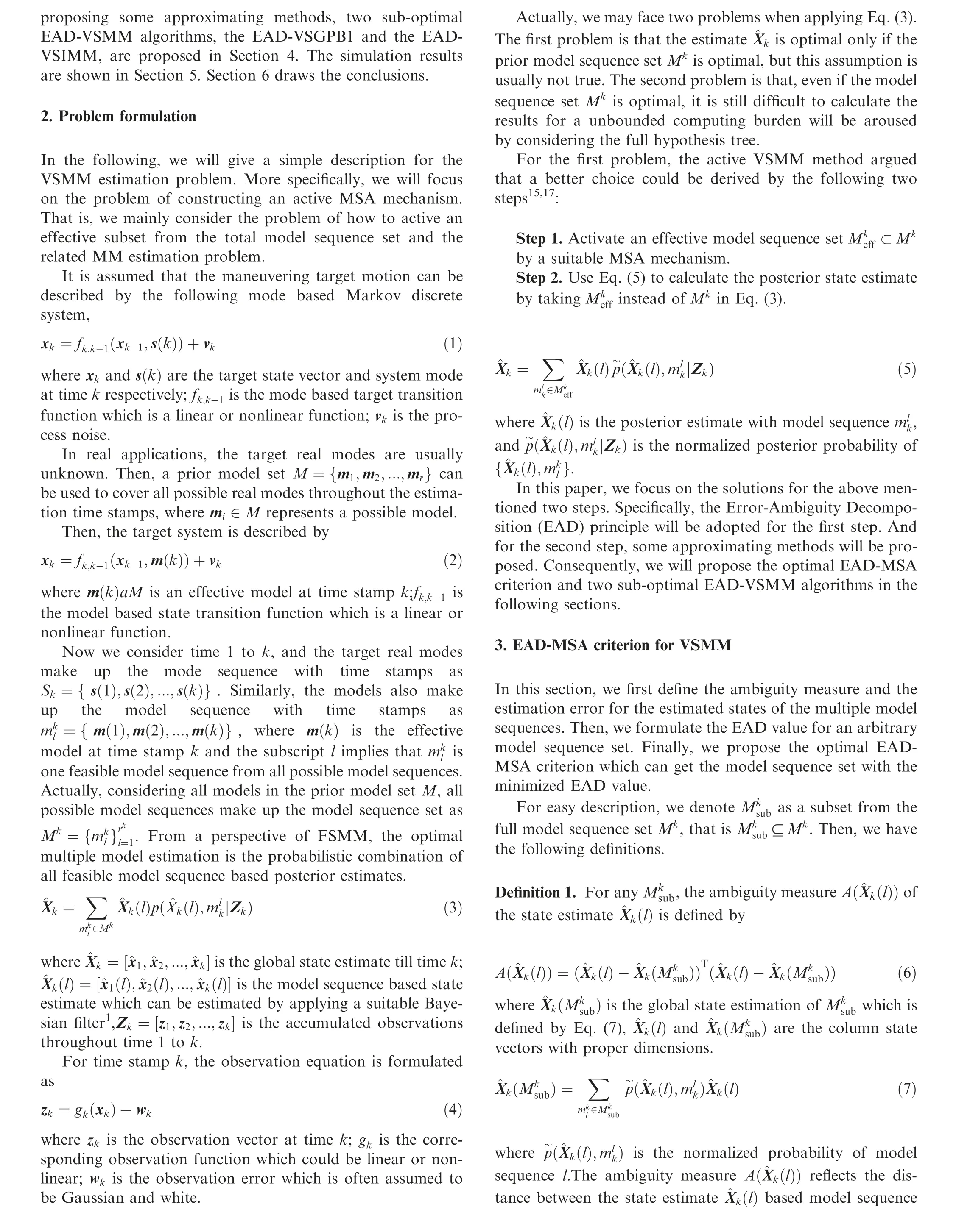
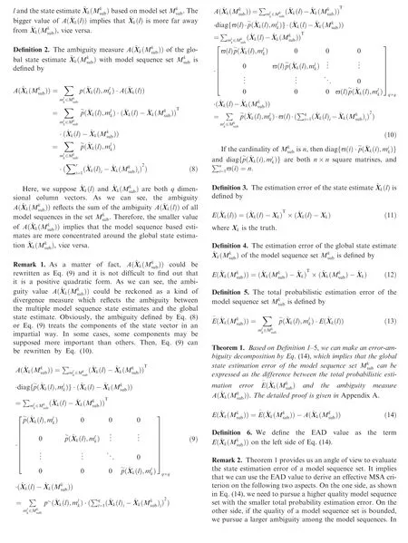
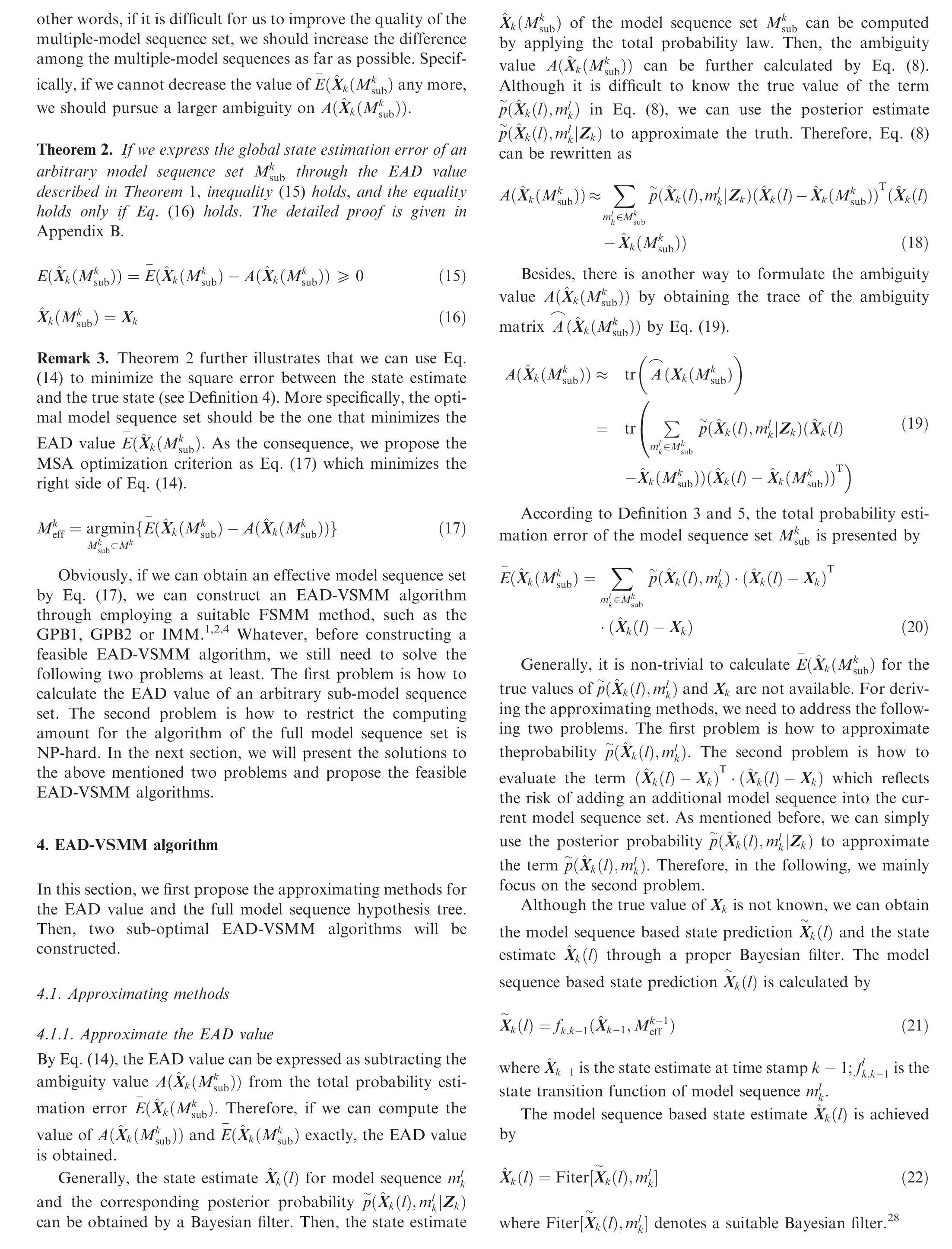
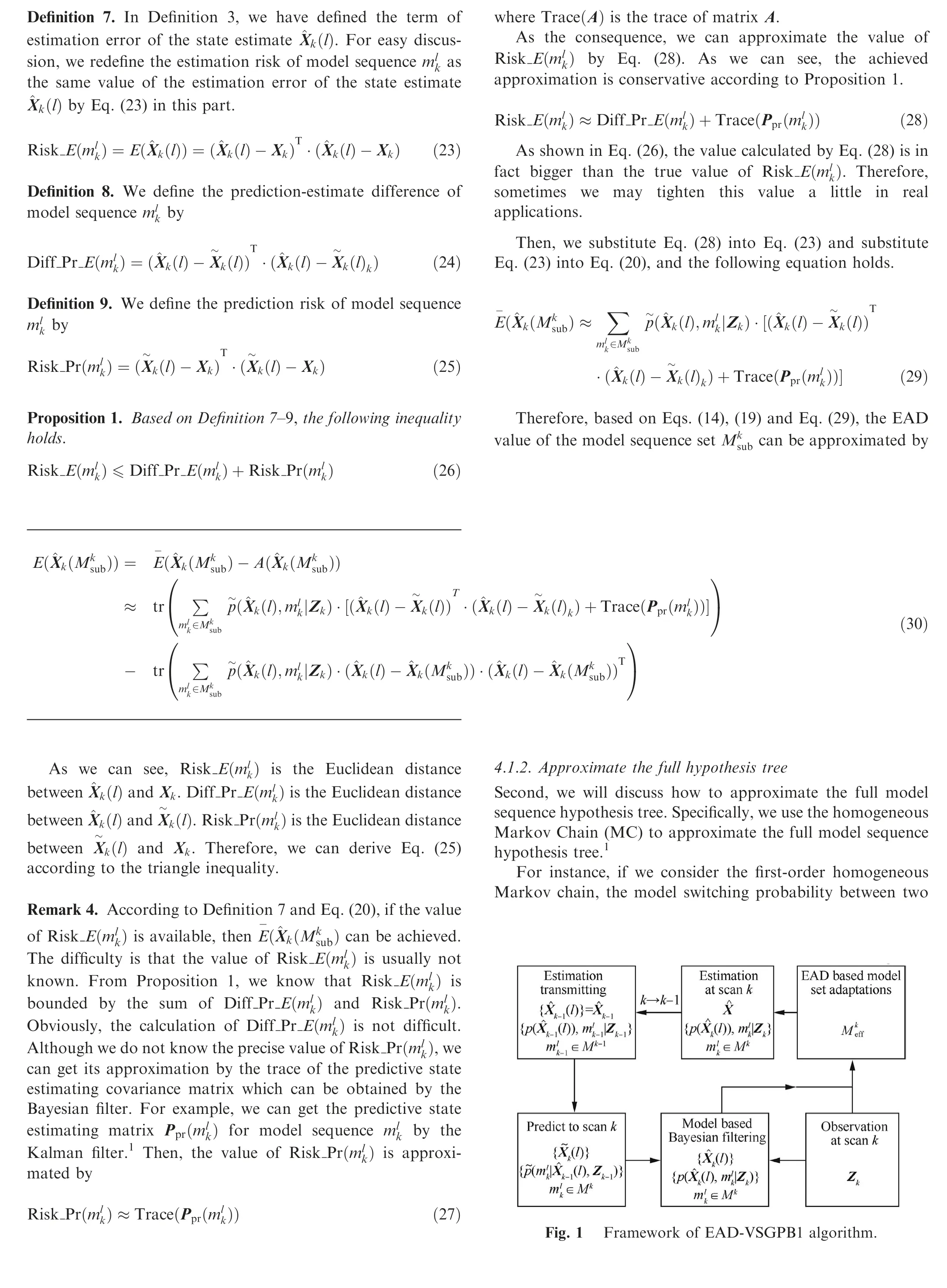
where aijdenotes the probability of p（mk（j）|mk-1（i）） where mk（j） means that the effective model at time stamp k is the jth model. For we can use Atransitionto approximate the full model sequence,many suboptimal approaches,such as the first and second Generalized Pseudo-Bayesian(GPB1,GPB2)algorithms or the IMM algorithm,1,2can be applied.Then,instead of considering the full hypothesis tree, we only need to handle a first- or second-order Markov chain.

4.2. EAD-VSGPB1 and EAD-VSIMM algorithms

In this section, we will propose two feasible EAD-VSMM algorithms. As described above, we can use Eq. (30) to calculate the EAD value and use Eq. (31) to approximate the full hypothesis tree. Then, the GPB1 and IMM methods are adopted into the EAD-VSMM framework, and the EADVSGPB1 and EAD-VSIMM algorithms are constructed.

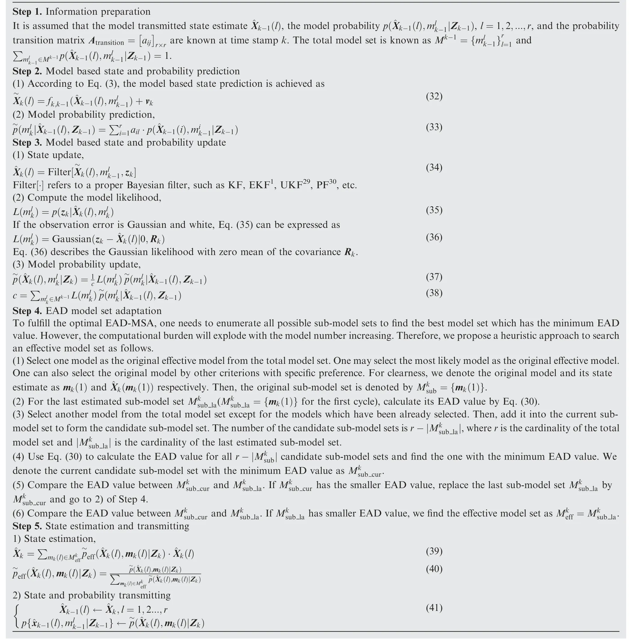
Table 1 One cycle of EAD-VSGPB1 algorithm.

The framework of the EAD-VSGPB1 algorithm is shown in Fig. 1. In the following part, we use l to denote the lth model rather than the lth model sequence. For instance, ^Xk（l） means the state estimate of model l at time stamp k.First,the predictions of the target state and the model probability at time stamp k can be achieved based on the state and model probability estimates at time stamp k-1.Second,we use the current observation zkto get the posterior state estimates of all models.Third, we use the EAD criterion to process the MSA. Finally,we obtain the target state estimate at time stamp k.A detailed description of the EAD-VSGPB1 algorithm is shown in Table 1.

IMM is a cost-efficient FSMM algorithm,so we adopted it into the EAD-VSMM framework to construct the EADVSIMM algorithm. The framework of EAD-VSIMM is similar to the framework of EAD-VSGPB1. The difference is that in the EAD-VSIMM we use the IMM algorithm to calculate the state and the model probability estimates, where in the EAD-VSGPB1 the employed algorithm is GPB1. A detailed description of the EAD-VSIMM algorithm is shown in Table 2.

5. Simulations

In this section, we apply the proposed EAD-VSGPB1 and EAD-VSIMM algorithms to the maneuvering target tracking scene. Then, we make the comparison among four existing algorithms (IMM,13LMS,17AMGEMM19and CS30,31) and the proposed algorithms (EAD-VSGPB1 and EADVSIMM). For clarity, we track a maneuvering target in the two-dimensional space. For providing fair results, we design two groups of tests. In the first group, two target mode determined scenarios will be considered. In the second group, we consider four random mode scenarios. Besides, all tests are achieved by 1000 Monte Carlo runs.

The target dynamics are described by the following linear equation:

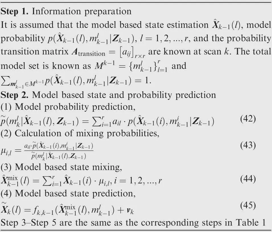
Table 2 One cycle of EAD-VSIMM algorithm.

where X（k）=［x1（k），x2（k），y1（k），y2（k）］Tis the target state at time k, and the components are the target position and the velocity along the x and y direction respectively;Acc（k）=［ax（k），ay（k）］Tis the dynamic mode, and the components are the accelerations along the x and y direction respectively;the sampling duration is 1 second and the contents of F and D are as follows:

The observation equation is

where Y（k）=［x1（k），y1（k）］Tis the observation vector of the target position along two coordinates, and W（k）=［wx（k），wy（k）］Tis the observation error which is assumed to be a zero mean Gaussian white process with prior known covariance matrix R. The prior model set includes 21 models, and each model describes a candidate target accelerating models. The details are as follows:m1=［0，0］T,m2，3=［0，±10］T,m4，5=［±10，0］T, m6，7，8，9=［±10，±10］T,m10，11=［0，±20］T, m12，13=［±20，0］T, m14，15，16，17=［±20，±20］T, m18，19=［0，±40］T, m20，21=［±40，0］T.

5.1. The first test group

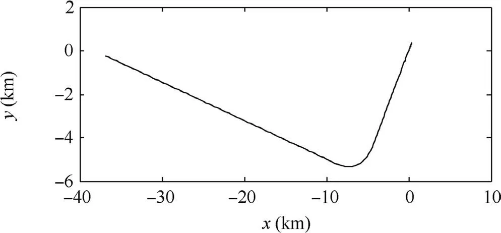
Fig. 2 Target trace.

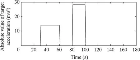
Fig. 3 Absolute value of target acceleration.

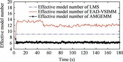
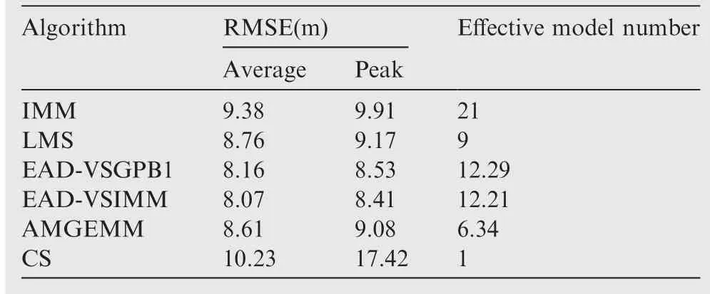
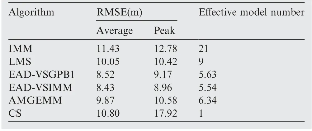
In the first test group, the mode determined maneuvering target was considered. The initial target state was X（1）=［100 m， 10 m/s， 100 m， 10 m/s］T. The entire tracking duration was 180 s and the scanning period was 1 s. In the moving duration, the target will perform two maneuvers: the first maneuver took place from time stamp 31 to 60, with a moderate maneuvering mode m9=［-10 m/s2，-10 m/s2］T,and the second one took place from time stamp 81 to 100,with a high maneuvering mode m16=［-20 m/s2，20 m/s2］T. In the remaining time, the target moved with the constant velocity mode. The target trace is shown in Fig. 2 and the absolute value of its acceleration is shown in Fig. 3. Four algorithms were tested in two scenes with different observation error magnitudes (R（1）=diag｛122m2，122m2｝ and R（2）=diag｛1202m2，1202m2｝). The detailed information of the tests is shown in Table 3. The Root-Mean-Square Error(RMSE) of Test 1 and 2 of four testing algorithms are shown in Figs.4 and 5 respectively,and the effective model number of Test 1 and 2 of the LMS algorithm,the AMGEMM algorithm and the proposed EAD algorithms are shown in Figs. 6 and 7 respectively. The detailed results of the estimation accuracy of Test 1 and 2 are listed in Tables 4 and 5 respectively. The detailed results of the effective model number of Test 1 and 2 of the LMS algorithm and the proposed EAD algorithms are listed in Tables 6 and 7 respectively.

As depicted in Fig.4 and Table 4,in Test 1(the determined maneuvering scene with small observation error), the best algorithms were the proposed EAD algorithms and the worst was the IMM algorithm. Specifically, when the target took a non-maneuvering mode(scan 3-30,scan 61-80 as well as scan 101-180), the five algorithms showed similar performance.When the target took weak maneuvering modes (scan 31-60), the VSMM algorithms showed better results than the IMM algorithm and the EAD algorithms were the best.When the target took strong maneuvering modes, the EAD algorithms performed much better than other algorithms.Comparing Fig. 4 with Fig. 6, we can see through pursuing the minimum EAD value, the EAD algorithms can adjust the effective model number adaptively. To our surprise, the EAD algorithms trended to use more models when the target

Table 3 Detailed information of test group one.

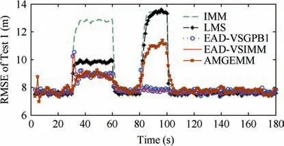
Fig. 4 RMSE of five algorithms in Test 1.

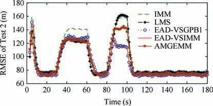
Fig. 5 RMSE of five algorithms in Test 2.

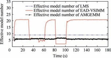
Fig. 6 Effective model number of LMS/AMGEMM/EAD algorithms in Test 1.

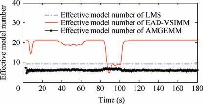
Fig. 7 Effective model number of LMS/AMGEMM/EAD algorithms in Test 2.

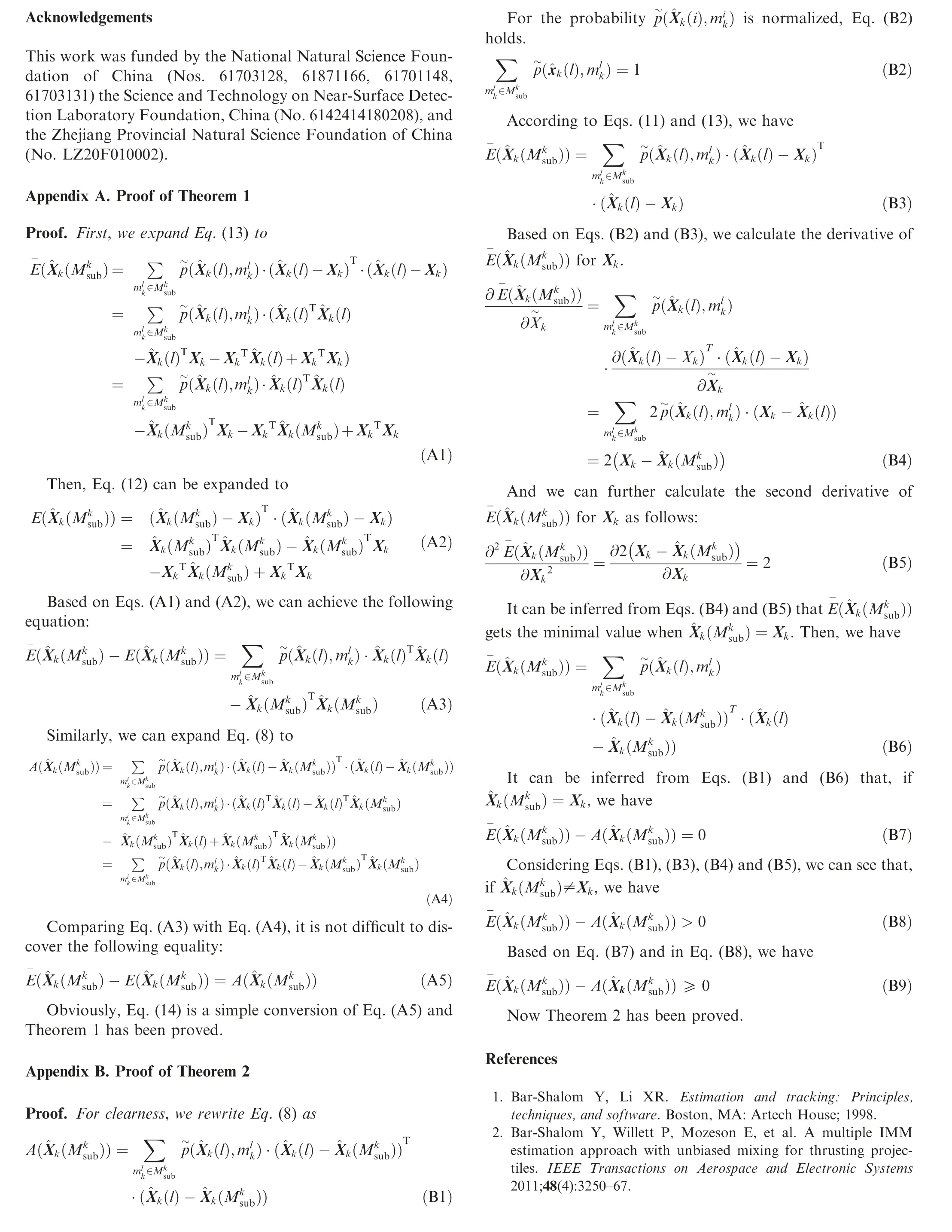
performed a non-maneuvering mode, and to use less models when the target performed strong maneuvering modes. We think that the reason is as follows. According to Theorem 1(Eq.(13)),the EAD value reflects the risk of adopting a model sequence set (the total probability estimation error) minus the corresponding ambiguity measure. When the target takes the non-maneuvering mode, the true mode is at the centrum of the prior model set. If we add more models into the effective model set in a symmetric way, the fused model will be not far away from the centrum (true mode). In such cases, adopting more models will help to get a smaller EAD value for the corresponding total probability estimation error is smaller than the ambiguity. If the target takes a strong maneuvering mode, the true mode goes to the border of the prior modelset, and adding an inaccurate model may bring a larger risk than the ambiguity measure. Therefore, adopting less models will help to get a smaller EAD value in such cases. Test 2 showed similar results (see Figs. 5, 7, Tables 5 and 7) to Test 1. For a larger observation error, the results of four testing algorithms got worse,and the EAD algorithms performed best and most robust.

Table 4 Detailed results of estimation accuracy of Test 1.

Table 5 Detailed results of estimation accuracy of Test 2.

Table 6 Detailed results of effective model number of Test 1.

Table 7 Detailed results of effective model number of Test 2.

5.2. The second test group

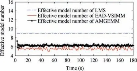
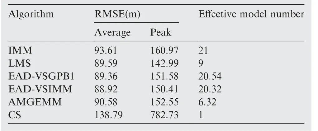
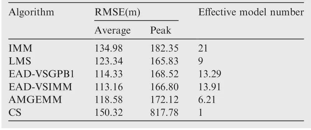
The second test group is very similar to the first test group.We still set the initial target state as X（1）=［100 m， 10 m/s，100 m， 10 m/s］T. The target also performs two maneuvers in the tracking duration:the first maneuver took place from time stamp 31 to 60, with a moderate maneuvering mode, and the second one took place from time stamp 81 to 100,with a high maneuvering mode.The small change we made here is that the target’s maneuvering modes are not the models in the prior model set.The detailed information of test group two is shown in Table 8. The Root-Mean-Square Error (RMSE) of Test 3 and 4 of four testing algorithms are shown in Figs. 8 and 9 respectively, and the effective model number of Test 3 and 4 of the LMS algorithm,the AMGEMM algorithm and the proposed EAD algorithms are shown in Figs. 10 and 11 respectively. The detailed results of the estimation accuracy of Test 3 and 4 are listed in Tables 9 and 10 respectively.The detailedresults of the effective model number of Test 3 and 4 of the LMS algorithm and the proposed EAD algorithms are listed in Tables 11 and 12 respectively.

Table 8 Detailed information of the second test group.

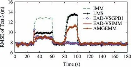
Fig. 8 RMSE of five algorithms in Test 3.

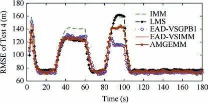
Fig. 9 RMSE of five algorithms in Test 4.

It can be concluded from the above tests’ results that the multi-model algorithms are still effective even the target’s real modes are not the models of the prior model set.We think that the reason is as follows. Although the real mode does not belong to the prior model set, several prior models with suitable weights can approximate the true mode well if the real mode is in the model space described by the prior model set.And the proposed EAD algorithm is the best and most robust one in the tested algorithms.

5.3. The third test group

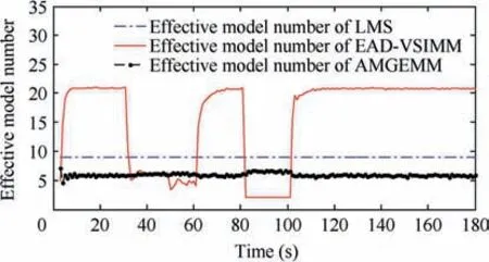
Fig. 10 Effective model number of LMS/AMGEMM/EAD algorithms in Test 3.

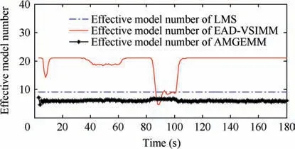
Fig. 11 Effective model number of LMS/AMGEMM/EAD algorithms in Test 4.

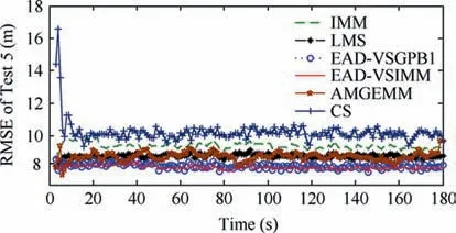
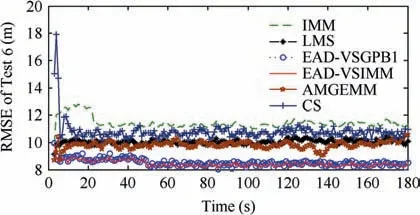
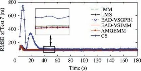
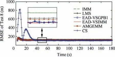
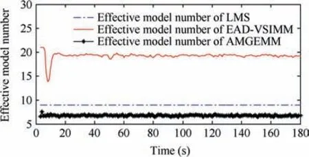
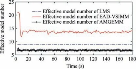
In the third test group, a mode undetermined maneuvering target was considered. The initial target state was still set to be X（1）=［100 m， 10 m/s， 100 m， 10 m/s］T.The entire tracking duration was 180 s and the scanning period was 1 s.In the tracking scene, the target started with a non-maneuvering mode, and then the target took a maneuvering mode stochastically. For instance, in a particular time stamp, we can set a probability of a for the non-maneuvering target to perform a maneuver(0

Table 9 Detailed results of estimation accuracy of Test 3.

Table 10 Detailed results of estimation accuracy of Test 4.

Table 11 Detailed results of effective model number of Test 3.

Table 12 Detailed results of effective model number of Test 4.

Table 13 Detailed information of test group three.

Fig. 12 RMSE of six algorithms of Test 5.

Fig. 13 RMSE of six algorithms of Test 6.

Fig. 14 RMSE of six algorithms of Test 7.

Fig. 15 RMSE of six algorithms of Test 8.

Fig. 16 Effective model number of LMS/AMGEMM/EAD algorithms in Test 5.

Fig. 17 Effective model number of LMS/AMGEMM/EAD algorithms in Test 6.

Fig. 18 Effective model number of LMS/AMGEMM/EAD algorithms in Test 7.

Fig. 19 Effective model number of LMS and proposed EAD algorithms in Test 8.

Table 14 Detailed results of estimation accuracy and effective model number of Test 5.

Table 15 Detailed results of estimation accuracy and effective model number of Test 6.

In the third test group,we tracked the target with different maneuvering probabilities and observation error magnitudes.The following conclusion can be inferred from Figs. 12-19 and Tables 14-17. First, the EAD algorithms are more robust and accurate than the LMS, AMGEMM, IMM and CS algorithms, especially when the target took more frequent maneuvers. Second, the EAD algorithms outperformed other tested algorithms when facing the big observation errors. Third, the EAD algorithms tend to use more models when facing weak maneuvers and big observation errors,while to use few models when facing strong maneuvers and small observation errors.Besides, the most vulnerable scene for the EAD algorithm was a weak maneuver and big observation error scene (just as the scene of Test 5). In such scenes, it is difficult to distinguish the model error deduced observation fluctuation from the observation error deduced observation fluctuation. Then,it is difficult to evaluate the risk of the model sequence set.Therefore, how to calculate the EAD value in a more proper way is a potential direction of future work.

Simple computational complexity analyses of the test algorithms are given in Table 18 where r is the total model number of the prior model set, K is the calculation scale of the employed Bayesian filter, λ is the effective model number for LMS and η is the particle number for AMGEMM.Therefore,among the test algorithms, CS is the simplest one and AMGEMM may consume more computing resources than others.The proposed algorithms consume a bit more comput-ing resources than the IMM and LMS algorithms if the total model number is not too large.

Table 16 Detailed results of estimation accuracy and effective model number of Test 7.

Table 17 Detailed results of estimation accuracy and effective model number of Test 8.

6. Conclusions

In this paper, the EAD principle has been adopted into the VSMM framework to formulate the EAD-MSA criterion.The EAD-MSA criterion is optimal in the sense of minimizing the square error between the state estimate and the true state.Specifically, the EAD value of a model sequence set can be decomposed as the total probability estimation error of the effective model sequence set minus the corresponding ambiguity measure,and the optimal model sequence set should be the one with the minimum EAD value.As the consequence,a useful principle is that, if it is difficult to achieve a more accurate model sequence set, we need to select a model sequence set with bigger ambiguity. For it is difficult to implement an optimal EAD-VSMM algorithm with limited calculation amount and partial observation, some approximating methods are designed and we propose two EAD-VSMM algorithms(EAD-VSGPB1 and EAD-VSIMM). Two groups of maneuvering target tracking scenes with different maneuvering modes and observation errors are tested. The simulation results demonstrate that the proposed EAD-VSMM algorithms outperform some benchmark MM algorithms in both accuracy and robustness.

Table 18 Simple computational complexity analyses of six algorithms.

3. Jo K, Chu K, Sunwoo M. Interacting multiple model filter-based sensor fusion of GPS with in-vehicle sensors for real-time vehicle positioning. IEEE Transactions on Intelligent Transportation Systems 2012;13(1):329-43.

4. Li XR,Jilkov VP.Survey of maneuvering target tracking—Part V:Multiple-model methods. IEEE Transactions on Aerospace and Electronic Systems 2005;41(4):1255-321.

5. Lainiotis DG. Optimal adaptive estimation: structure and parameter adaptation. IEEE Transactions on Automatic Control 1971;16:160-70.

6. Jilkov VP, Li XR. Online bayesian estimation of transition probabilities for Markovian jump systems. IEEE Transactions on Signal Processing 2004;52(6):1620-30.

7. Jaime LA, Angle JJ, Juan AB, et al. A new approach to mapassisted Bayesian tracking filtering. Information Fusion 2019;45:79-95.

8. Vasuhi S, Vaidehi V. Target tracking using interactive multiple model for wireless sensor network. Information Fusion 2016;27:41-53.

9. Garcia J, Besada JA, Molina JM, et al. Model-based trajectory reconstruction with IMM smoothing and segmentation. Information Fusion 2015;22:127-40.

10. Li XR, Bar-Shalom Y. Multiple-model estimation with variable structure. IEEE Transactions on Automatic Control 1996;41:478-93.

11. Dong P, Jing ZL, Gong D, et al. Maneuvering multi-target tracking based on variable structure multiple model GMCPHD filter. Signal Processing 2017;141:158-67.

12. Bar-Shalom Y, Willett PK, Tian X. Tracking and data fusion. CT: YBS; 2011.

13. Hayashi Y, Tsunashima H, Marumo Y. Detection of railway vehicles using multiple model approach. International Joint Conference; 2006. p. 2812-7.

14. Ho TJ. A switched IMM-extended viterbi estimator-based algorithm for maneuvering target tracking. Automatica 2011;47(1):92-8.

15. Li XR. Multiple-model estimation with variable structure—part II:model-set adaptation.IEEE Transactions on Automatic Control 2000;45:2047-60.

16. Wang L,Gao HT.A variable structure multiple model filtering for SINS/DVL integrated solution. Proceedings of the 2017 Chinese control conference. p. 26-8.

17. Dong P, Jing ZL, Gong DR, Tang BT.Maneuvering multi-target tracking based on variable structure multiple model GMCPHD filter. Signal Processing 2017;141:158-67.

18. Li XR, Zhi XR, Zhang YM. Multiple-model estimation with variable structure—Part III: Model-group switching algorithm.IEEE Transactions on Aerospace and Electronic Systems 1999;35:225-41.

19. Li XR, Zhang YM. Multiple-model estimation with variable structure part V:likely-model set algorithm.IEEE Transactions on Aerospace and Electronic Systems 2005;36(2):448-66.

20. Shen-tu H, Xue AK, Guo YF. Feedback structure based entropy approach for multiple-model estimation. Chinese Journal of Aeronautics 2013;26(6):1506-16.

21. Shen-tu H,Xue AK,Peng DL.Geometrical entropy approach for variable structure multiple-model estimation. Chinese Journal of Aeronautics 2015;28(4):1131-46.

22. Li XR,Jilkov VP,Ru JF.Multiple-model estimation with variable structure part VI: expected-mode augmentation. IEEE Transactions on Aerospace and Electronic Systems 2005;41(3):853-67.

23. Lan J, Li XR. Equivalent-model augmentation for variablestructure multiple-model estimation. IEEE Transactions on Aerospace and Electronic Systems 2013;49:2615-30.

24. Xu LF, Li XR, Duan ZS. Hybrid grid multiple-model estimation with application to maneuvering target tracking. IEEE Transactions on Aerospace and Electronic Systems 2016;52(1):122-36.

25. Krawczyk B, Minku LL, Woniak M. Ensemble learning for data stream analysis. Information Fusion 2017;37:132-56.

26. Tekin C, Yoon J, Schaar MVD. Adaptive ensemble learning with confidence bounds. IEEE Transactions on Signal Processing 2015;65:888-903.

27. Krogh A, Vedelsby J. Advances in Neural Information Processing Systems. Massachusetts: MIT Press; 1995.

28. Zhou ZH. Ensemble methods: Foundations and algorithms. Boca Raton: CRC Press; 2012.

29. Li L,Xia YQ.UKF-based nonlinear filtering over sensor networks with wireless fading channel. Information Sciences 2015;316:132-47.

30. Wu JF, Li G. Research on target tracking algorithm using improved current statistical model.IEEE 2nd advanced information technology, electronic and automation control conference; 2017. p.2515-7.

31. Sun W, Yang YJ. Adaptive maneuvering frequency method of current statistical model.IEEE/CAA Journal of Automatica Sinica 2017;4(1):154-60.