Fault diagnosis of chemical processes based on partitioning PCA and variable reasoning strategy☆

Guozhu Wang *,Jianchang Liu Yuan Li,Cheng Zhang

1 College of Information Science and Engineering,Northeastern University,Shenyang 110819,China

2 State Key Laboratory of Synthetical Automation for Process Industries,Northeastern University,Shenyang 110819,China

3 Information Engineering School,Shenyang University of Chemical Technology,Shenyang 110142,China

1.Introduction

Detection and identification of abnormal operating condition are very important for safety and efficient operations in chemical processes.With the fast development of chemical process control and computer application technology,large amount of process data can be obtained online using sensors[1],making data-driven methods available for process monitoring and fault variable recognition.As a key technique,data-based process fault detection and identification methods have attracted lots of attentions in the past years.Some fault detection and isolation methods have been developed and become popular,such as principal component analysis(PCA),partial least squares(PLS),and their extensions[2–17].Various ideas have been proposed and studied[18–25],which may be classified into three categories in general[26–29]:based on quantitative model,qualitative model,and hybrid model.Quantitative model-based methods usually need precise mathematical model,which is difficult to build for complex chemical process.Qualitative model-based methods employ cause–effect reasoning to describe system behavior such as fault trees and signed digraph analysis methods,but these methods are restricted to systems with relatively small number of variables or states because the creation of knowledge base is timeconsuming[30].Hybrid model method is a comprehensive fault monitoring and identification method,which has some achievements with data and experience of process,but it is difficult to obtain experiences and knowledge of process in a short term.

With the accuracy requirement in the process monitoring,several methods based on data driven were studied such as hierarchical and multi-block statistical[21,31,32].MacGregor et al.proposed monitoring and diagnosis charts for sub-blocks and a global monitoring chart for performance enhancement[18].Westerhuis et al.provided a comprehensive analysis for several multi-blocks and hierarchical PCA and PLS algorithms in a unified notation[19].The multi-block,hierarchical PCA and PLS algorithms were also analyzed,Qin et al.defined block and variable contributions to make monitoring process decentralized[20].Smilde et al.proposed a sequential multi-block componentmethod and reviewed several sequential multi-block methods[21].Ge et al.proposed a two-step multi-block monitoring method[33]improving the monitoring performance and fault interpretation effectively.Recently,some popular methods were studied,which are different from the traditional methods and more reliable for fault diagnosis[34–36].However,some process knowledge of block and hierarchy division is needed for almost all of these methods,which isa key step and affectsmodeling accuracy.Actually itis very difficultto obtain usefulprocess knowledge in complex chemical environment,so pure block division methods based on data are needed.

After a fault is detected,it is desirable to identify its roots from possible fault variables or locate fault sensors.Contribution plot[37]can find the fault variable with high contribution.Kourti and MacGregor applied contribution plots for quality and process variables to find fault variables of a high-pressure low-density polyethylene reactor[38].They pointed out that the contribution plots may not reveal the assignable causes of abnormal events.One reconstructionbased approach was designed for isolating fault variables from the subspaces of faults[39].This method was applied to reconstruct data of fault variables before a prediction for a soft sensor model[40].Yue and Qin developed a combined index of Q and T2to isolate fault variables[34],and obtained a more feasible solution from reconstruction-based approach[39].The reconstruction based contribution(RBC)approach was derived[41],which may not suffer the smearing effect as the contribution plots of PCA.In reality,the smearing effect of RBC could be observed when implementing the confidence intervals of RBC plots,since the control limits were derived based on normal operating data,which cannot guarantee that the magnitude of fault variables smearing over the non-faulty ones would be under the control limits[42].However,it is well known that the smearing out of contributions leads to misdiagnose fault variables.Wang et al.proposed a fault diagnosis method using kNN reconstruction on MRI variables and improved the fault recognition effect[43],but they rarely considered the correlation between variables.Qin gave a brief survey on the methods for data-driven industrial process monitoring and diagnosis[44].Recently,Xu et al.proposed a new weighted reconstruction-based contribution for improved fault diagnosis,which could reduce fault coefficient smearing and improve diagnosis accuracy adaptively[45].

In this paper,a partitioning PCA(PPCA)method is developed to partition blocks and detect fault.First,the PCA methodology is applied to initial data and transforms the high dimensional input space into lower dimensional subspaces while retaining the salient characteristics of measured variables.Uncorrelated principal components can be obtained because different principal component directions are orthogonal with each other.Second,industrial processes are divided into several local models according to these uncorrelated directions.The subset of variables is selected according to their contributions to principal component directions in each local subset.Then the PPCA models are built in different local models,in which variables may overlap.This method has an advantage compared with PCA and global modeling ideas:it intends to examine the process change in different monitoring directions,so that the fault can be detected readily.

A variable reasoning strategy is introduced under the PPCA framework to locate a few fault variables simultaneously and eliminate some normal variables.This method can also give some initiatory judgment for ambiguous variables.

2.Process Monitoring Based on PPCA Method

We propose a novel fault detection method,PPCA.It includes two parts.(1)Selection of relevant variables in each sub-partitioning:divide original data set into several subsets,each principal component direction of PCA represents one subset,and residual subspace is seen as a whole.Then find representative variables in each sub-partitioning according to theircontributionsto corresponding principalcomponentdirection.(2)Process monitoring:build PPCA models using traditional PCA method for fault detection.

2.1.Selection of relevant variables

For a data set X∈Rn×m,n is the number of training samples and m is the numberofvariables orsensors.The PCAdecomposition[3]iscarried out on X first.

whereandrepresentthe principalpart and residualpart,andare score matrix and loading matrix of principal part,respectively,andbelong to residual part.

The original space is divided into two subspaces:principal component subspace(PCS)and residual subspace(RS).Therefore,the loading matrix contains PPCSand PRS,representing differentprincipaldirections,where PPCS=[p1,p2,…,pA]and PRS=[pA+1,pA+2,…,pm].

As an essential parameter,the number of principal components A is selected by employing cumulative percent variance(CPV)method[46,47].Because all of the principal components are orthogonal with each other,when we select the most relevant variables in each principal component direction,the multiple partitioning is acquired.The selection method of relevant variables is described as follows.

For PCS,itis easy to obtain the contribution of each variable in different directions

whereis the contribution of variable i to principal component direction j.

For RS,an independent local partitioning can be established when we consider it as a whole,in which the contributions of relevant variables are:

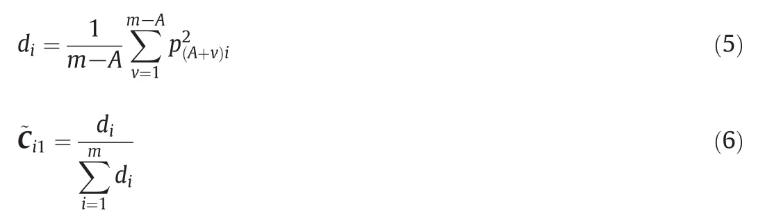
whereis a vector,and each elementrepresents the mean value ofthe contribution of each variable to RS.

After determiningand,A+1 partitionings can be obtained through dividing original data,and the contribution of all variables in each local direction is

The contribution value of each variable can be sorted in descending order for the corresponding direction,and those variables with high contribution values should be retained.In addition,to ensure that no variable is missing,variable set of different directions should include all variables in the system.A variable selection rule can be described as

where Si(V)is the selected variable set in the i th partitioning and S(V)contains all variables in industrial process.

2.2.Fault detection based on PPCA method

Variables can be retained according to Eqs.(7)and(8)for each partitioning,all variables are divided into A+1 parts,and each part contains higher contribution variables in its direction.However,some same variables can be assigned to differentparts when they have higher contribution in different directions.For example,for a system containing eightvariables and 2 principalcomponents,three localpartitionings can be constructed:(1)X1={v2,v3,v5,v7},containing variables 2,3,5 and 7;(2)X2={v3,v4,v6,v8};and(3)X3={v1,v2,v4,v5}.Xiretains those variables with high contribution values in the corresponding direction.Because variable 2 has higher contribution in two partitionings,it is retained in partitionings 1 and 3.

Individual PPCA model can be developed as follows.According to Section 2.1,it is possible to decompose original data set Xn×minto multiple local subsets X1,X2,…,XA,XA+1.Then PCA is applied in each partitioning.

where Xirepresents the i th partitioning data set.

In order to judge if the SPE and T2values are larger than normal threshold,the control limit(SPELim,iand T2Lim,iof each partitioning model are necessary,which are calculated similar to the traditional PCA method[3,17]as follows.

SPE confidence limit:

where i is the label of local partitioning,Aiis the number of principal component in the i th partitioning PCA model and is calculated by employing CPV method,(λj)iis the j th eigenvalue of covariance matrixand miis the dimension of Xi.

T2confidence limit:

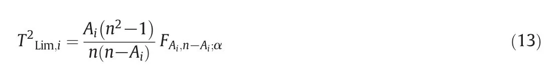
where n is the number ofsamples,FAi,n−Ai;αis an F distribution with degrees of freedom Aiand n − Ai,and α is the confidence level[3,17].

A new sample x is standardized and divided into A+1 parts:x1,x2,…,xA,xA+1;and then xiis projected into corresponding local model,

where Λi=diag[(λ1)i,(λ2)i,…,(λAi)i].

Under normal circumstances,SPEiand Ti2are smaller than SPELim,iand T2Lim,i,respectively.If the value of SPEior Ti2increases suddenly at some points,the system is out of order.Because this method intends to examine the process change in different monitoring directions,the fault can be detected more easily.

3.Fault Identification Based on Variable Reasoning Strategy

Once faults are detected,we must find the fault roots and exclude them as soon as possible.Traditional variable contribution plot[37,48]has some ability for fault identification by computing and comparing contribution indexes of process variables.Process variable with the highest contribution to the monitoring statistic index can be identified,and this variable may be the most possible reason of fault.Since the number of process variables is always very large in complex chemical processes,it is impossible that all fault variables are identified through contribution plot method.Moreover,this method may lead to misdiagnose fault variables[42,49].The variable reasoning strategy is a novel fault identification and location method based on partitioning PCA,giving initiatory judgment for all variables.

In the PPCA monitoring system,when a fault is detected in several local partitioning models,we can divide A+1 independent local sets into two groups,fault set Fs and normal set Ns.

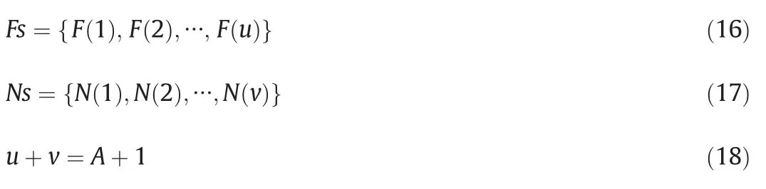
where u and v are the sizes of two sets,and Fs includes all local partitioning models that are faulty.For normal variable set NV,doubtless faultvariable set FV,and uncertain faultvariable set UFV,the following reasoning is effective.

where V(N(j))are all variables in the j th normal local partitioning model,V includes all variables in the system,and FV is the set of all faultvariables.There are two methods to determine FV.One is the traditional variable contribution plot.Contribution indexes of process variables in each fault local monitoring process are computed and compared,the variable with the highest contribution is retained,and these variables should be contained in FV.Another method is the exclusion of variables.When all normal variables are excluded,if only one variable is retained in F(i),it must belong to FV.

4.Case Studies

In this section,two cases are used to demonstrate the process monitoring and fault identification performance of the proposed method.First,a numerical example is adopted,and it aims at recognizing several faultvariables simultaneously.Then the method is applied in Tennessee Eastman chemical process and compared with PCA,KPCA,ICA and kNN methods.

4.1.Numerical example

A numerical example is redesigned for specific purpose in this work.The example contains five variables driven by two factors,s1:uniform(−10,−7)and s2:N(−15,1).The simulation data are generated from the following equations:

Fig.1.Monitoring results of traditional PCA method.

where e1–e5are zero-mean white noises with a standard deviation of 0.01.

500 samples are simulated to constitute the normaltraining data set.To illustrate the fault detection and recognition performance,several faults are added to the process variables as follows:for variable v1,a fault is added,which is 30%of its variation range between 51 and 100 samples;for variable v2,added fault is 20%of its variation range between 301 and 350 samples;for variables v3and v4,added faults are 8%and 10%of their variation range between 301 and 350 and 51 and 100 samples,respectively.In modeling phase,the number of principal components is determined by the cumulative percentage of explained variance(85%).One principal component is selected for the PCAmodel,which can explain 96.7%of the process information in this system.

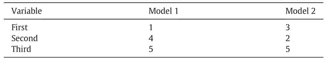
Table 1 Relevant variables of each local model

Fig.1 gives the traditional PCA monitoring results for comparison.Since the number of principal component is 1,two PPCA models can be constructed in this system.Each model contains three variables selected based on the contribution of each variable.The results of variable selection are given in Table 1.The numbers of principal components of the two models are A1=1 and A2=2.Process monitoring results based on PPCA are shown in Fig.2.The SPE fault detection results of two methods are consistent approximately,while T2of PPCA is better than that of PCA.The faults can be detected from 51 to 100 samples in model 1,while model 2 is effective for the fault from 301 to 350 samples.In short,PPCA method can detect the fault of all time effectively.

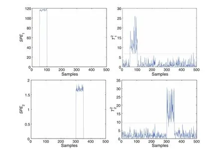
Fig.2.Monitoring results of PPCA method.

Fig.3.The contributions of variables at 51 and 301 samples.

Table 2 The results of fault diagnosis

For the fault variable identification,traditional contribution plot method confirms that the largest contribution variable is faulty,but it is difficult to give judgment for other variables.As shown in Fig.3,variables 1 and 3 can be considered as the fault variables at 51 and 301 samples,respectively.Variable 4 has higher contribution at 51 and 301 samples,but we are not sure that it is the fault variable,which is the disadvantage of traditional contribution plot method.However,the PPCA method can give some initiatory judgment for all variables.In Fig.2,model 1 is effective from 51 to 100 samples,so the most likely fault variables are 1,4,and 5.Between 301 and 350 samples,the most likely fault variables are 2,3,and 5.Oppositely,variables 1,4,and 5 are normal between 301 and 350 samples,while variables 2,3,and 5 are normal between 51 and 100 samples,where variable 5 is superimposed in two models.Furthermore,the contribution indexes of process variables can be computed and compared in order to find the fault variables accurately.The result of diagnosis is shown in Table 2.

4.2.TE chemical benchmark

The well-known Tennessee Eastman process has been widely applied to evaluate the effectiveness of process monitoring techniques,which is a simulation of the practical chemical process[50–52].There are five major unit operations in the TE process:a reactor,a condenser,a compressor,a separator and a stripper.The control structure is shown in Fig.4.For process monitoring purposes,33 variables are selected,including 11 manipulated variables and 22 continuous process variables,as shown in Table 3.As training data,960 samples are generated for training PPCA model.21 fault data sets are generated for testing purpose.Each fault data set includes 960 samples,and all faults are introduced at sample 161.The descriptions of 21 faults are given in Table 4,where,faults 16–20 are unknown faults.To build PPCA monitoring model,an initial PCA decomposition is carried out.Depending on the CPV rule,the number of principal components is 14,which can explain 88.2%ofthe process information.Hence,a totalof15 models can be constructed in this system,and 5 variables are selected in each local model to ensure that models contain all process variables.The result is expressed in Table 5.

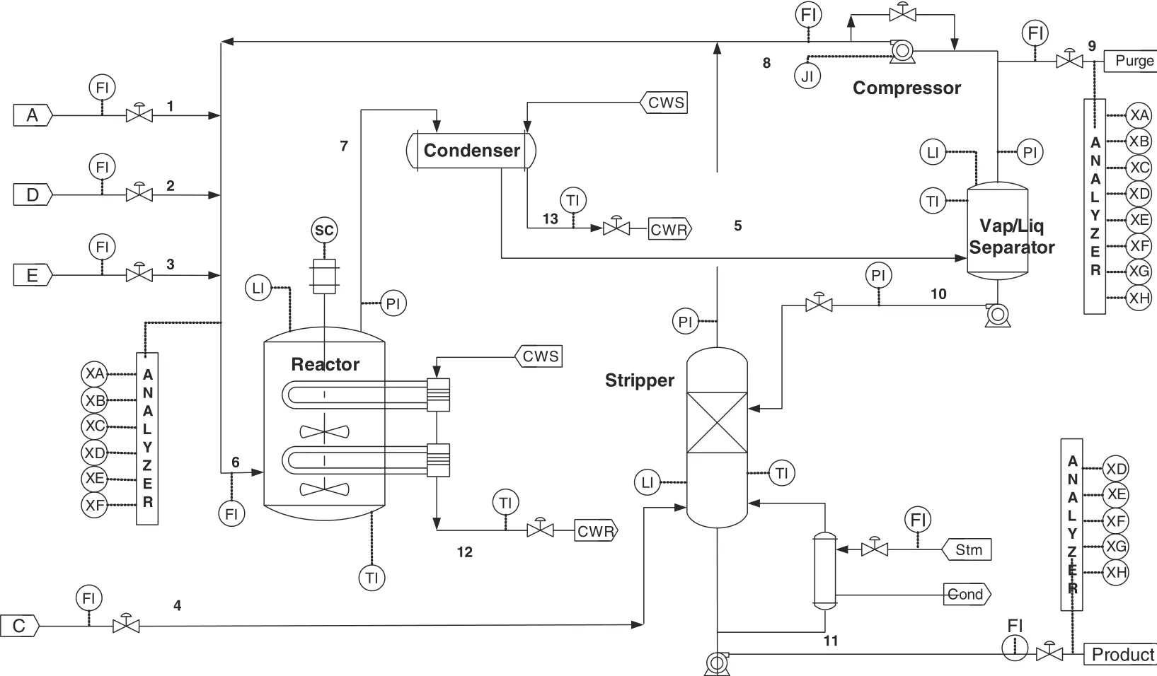
Fig.4.Process flow diagram of the Tennessee Eastman chemical process.

Table 3 Monitoring variables in the TE process

Table 4 Fault description of TE process

Table 5 Relevant variables of each local model

For comparison,the PCA,KPCA,ICA and kNN monitoring results for fault 5 are given in Fig.5.The fault cannot be discovered in time,and the fault cannot be detected accurately all the time from the correlation between variables.However,the proposed method can detect the fault once a local model finds.Several monitoring results for fault 5 based on PPCA method are shown in Fig.6.Comparing the monitoring results in Figs.5 and 6,we can see that the performance of PPCA is improved greatly especially in local models 4,7,9,10 and 13.For example,the fault detection results of the traditional methods are not satisfactory after the four hundredth sample,and they can be detected hardly in T2model.With PPCA,the detection results of local models 4,7,and 9 are superior.The fault is hardly detected in model 6,and the corresponding responsible variables in this model include variables 15,30,12,29 and 17,which are stripper level,stripper liquid product flow valve,product separator level,separator pot liquid flow valve,and stripper under flow.These five variables should be included in NV.To find the most possible fault variables,we exclude normal variables from the fault models.Through above analysis,NV,FV and UFV of fault 5 can be obtained preliminary.

To illustrate how to identify fault variables or how to find NV,FV and UFV,the T2monitoring results of fault 1 from 910 to 920 samples are used as example.Since the number ofprincipalcomponents is 14,there are 15 monitoring results in Fig.7.The fault can be detected using models 1,4,7,10,11,12 and 13 at sample 915,while the monitoring results of models 2,3,5,6,8,9,14 and 15 are fault-free.Therefore,responsible variables in fault-free models are normal and NV can be determined at sample 915.According to the previous theoretical analysis,the lighter parts of Table 5 represent fault models containing suspected fault variables at sample 915(these models can detect the faults),and the darker parts are normal models composed of normal variables NV(the process is normal in these models).We can eliminate NV from the suspected fault variables,and Table 6 gives the key fault variables.Hence,the diagnosis results of fault 1 become clearer,and further summary is shown in Table 7.The doubtless fault variables include variables 14(product separator under flow)and 26(total feed flow valve).Variables 1,13,16,25 and 29 are the suspected fault variables,and the restis normal variables.In Table 8,the SPE and T2fault detection rates(the ratio of the number of detected fault to that of actual fault)of PCA,KPCA,ICA,kNN and PPCA methods are also given for comparison.The proposed method may be recognized because of its superiority in fault detection rates,which is a little better than the other methods.

5.Conclusions and Prospects

In this paper,a novel process monitoring and fault variable identification methods are proposed.This method can extract local information effectively through dividing observation data into several local models.For the process monitoring,the proposed method intends to monitor the process change in different directions,and it is earlier and more accurate than the traditional methods.For the fault identification,the variable reasoning strategy is different from the contribution plot.It not only locates the fault variables effectively,but also finds NV,FV and UFV of complex chemical processes conveniently.

This paper mainly focuses on process modeling,fault monitoring and identification,and it is effective for online and of fline systems.Some interesting issues will be multi-way PPCA for batch process monitoring,supervised learning-based PPCA for process fault identification and online fault monitoring and identification methods.Furthermore,it will be more useful when this method combines with additional fault diagnosis methods such as expert knowledge.

Fig.5.Monitoring results of fault 5.(a)PCA;(b)KPCA;(c)ICA;(d)kNN.

Fig.6.Monitoring results of fault 5 on models 2,3,4,6,7,9,10 and 13.

Fig.6(continued).

Fig.7.T2 monitoring results of fault 1 based on partitioning PCA method.

Table 6 Fault models and suspected fault variables at 915 sample

Table 7 The variable reasoning result based on PPCA at sample 915 for fault 1

Table 8 Monitoring results of 21 faults on TE process

[1]D.C.Montgomery,Introduction to statistical quality control,Wiley,New York,1991.

[2]J.Yu,J.Yu,Nonlinear bioprocess monitoring using multiway kernel localized fisher discriminant analysis,Ind.Eng.Chem.Res.50(6)(2011)3390–3402.

[3]J.Kresta,J.F.MacGregor,T.E.Marlin,Multivariate statistical monitoring of process operating performance,Can.J.Chem.Eng.69(1)(1991)35–47.

[4]P.Nomikos,J.F.MacGregor,Monitoring batch processes using multiway principal component analysis,AICHE J.40(8)(1994)1361–1375.

[5]T.Kourti,J.F.MacGregor,Process analysis,monitoring and diagnosis,using multivariate projection methods,Chemom.Intell.Lab.Syst.28(95)(1995)3–21.

[6]Y.W.Zhang,C.Ma,Fault diagnosis of nonlinear processes using multiscale KPCA and multiscale KPLS,Chem.Eng.Sci.66(1)(2010)64–72.

[7]G.Z.Wang,J.C.Liu,Y.W.Zhang,Y.Li,A novel multi-mode data processing method and its application in industrial process monitoring,J.Chemom.29(2)(2015)126–138.

[8]Y.Yao,T.Chen,F.Gao,Multivariate statistical monitoring of two-dimensional dynamic batch processes utilizing non-Gaussian information,J.Process Control 20(10)(2011)1188–1197.

[9]J.Wang,Q.P.He,Multivariate statistical process monitoring based on statistics pattern analysis,Ind.Eng.Chem.Res.49(17)(2010)7858–7869.

[10]Z.Q.Ge,C.J.Yang,Z.H.Song,Improved kernel PCA-based monitoring approach for nonlinear processes,Chem.Eng.Sci.64(9)(2009)2245–2255.

[11]J.Y.Guo,H.B.Chen,Y.Li,MPCA fault detection method based on multiblock statistics for uneven-length batch processes,J.Comput.Inf.Syst.9(18)(2013)7181–7190.

[12]X.Wang,U.Kruger,G.W.Irwin,G.McCullough,N.McDowell,Nonlinear PCA with the local approach for diesel engine fault detection and diagnosis,IEEE Trans.Control Syst.Technol.16(1)(2008)122–129.

[13]Y.H.Lee,H.D.Jin,C.H.Han,On-line process state classification for adaptive monitoring,Ind.Eng.Chem.Res.45(9)(2006)3095–3107.

[14]X.Z.Wang,S.Medasani,F.Marhoon,H.Albazzaz,Multidimensional visualization of principal component scores for process historical data analysis,Ind.Eng.Chem.Res.43(22)(2004)7036–7048.

[15]M.Kano,K.Nagao,H.Hasebe,T.Hashimoto,H.Ohno,R.Strauss,B.R.Bakshi,Comparison of multivariate statistical process monitoring methods with applications to the Eastman challenge problem,Comput.Chem.Eng.26(1)(2002)161–174.

[16]B.R.Bakshi,Multiscale PCA with applications to multivariate statistical process monitoring,AICHE J.44(7)(1998)1596–1610.

[17]J.E.Jackson,A user's guide to principal components,Wiley,New York,1991.

[18]J.F.MacGregor,C.Jaeckle,C.Kiparissides,M.Kourtoudi,Process monitoring and diagnosis by multiblock PLS methods,AICHE J.40(5)(1994)826–838.

[19]J.A.Westerhuis,T.Kourti,J.F.MacGregor,Analysis of multiblock and hierarchical PCA and PLS models,J.Chemom.12(5)(1998)301–321.

[20]S.J.Qin,S.Valle,M.J.Piovoso,On unifying multiblock analysis with application to decentralized process monitoring,J.Chemom.15(9)(2001)715–742.

[21]A.K.Smilde,J.A.Westerhuis,S.DeJong,A framework for sequential multiblock component methods,J.Chemom.17(6)(2003)323–337.

[22]G.Z.Wang,J.C.Liu,Y.Li,L.L.Shang,Fault detection based on diffusion maps and k nearest neighbor diffusion distance of feature space,J.Chem.Eng.Jpn.48(9)(2015)756–765.

[23]M.A.Hussain,C.R.Che Hassan,K.S.Loh,K.W.Mah,Application of artificial intelligence technique in process fault diagnosis,J.Eng.Sci.Technol.2(3)(2007)260–270.

[24]H.Guo,H.G.Li,On-line batch process monitoring with improved multi-way independent component analysis,Chin.J.Chem.Eng.21(3)(2013)263–270.

[25]X.Deng,X.Tian,Multimode process fault detection using local neighborhood similarity analysis,Chin.J.Chem.Eng.22(11)(2014)1260–1267.

[26]V.Venkatasubramanian,R.Rengaswamy,K.Yin,S.N.Kavuri,A review of process fault detection and diagnosis:Part I:Quantitative model-based methods,Comput.Chem.Eng.27(3)(2003)293–311.

[27]V.Venkatasubramanian,R.Rengaswamy,S.N.Kavuri,A review of process fault detection and diagnosis:Part II:Qualitative models and search strategies,Comput.Chem.Eng.27(3)(2003)313–326.

[28]V.Venkatasubramanian,R.Rengaswamy,S.N.Kavuri,K.Yin,A review of process fault detection and diagnosis:Part III:Process history based methods,Comput.Chem.Eng.27(3)(2003)327–346.

[29]F.Yang,P.Duan,S.L.Shah,T.Chen,Capturing connectivity and causality in complex industrial processes,Springer,2014.

[30]C.K.Lau,K.Ghosh,M.A.Hussain,C.R.Hassan,Fault diagnosis of Tennessee Eastman process with multi-scale PCA and ANFIS,Chemom.Intell.Lab.Syst.120(2)(2013)1–14.

[31]S.W.Choi,I.B.Lee,Multiblock PLS-based localized process diagnosis,J.Process Control 15(2005)295–306.

[32]G.A.Cherry,S.J.Qin,Multiblock principal component analysis based on a combined index for semiconductor fault detection and diagnosis,IEEE Trans.Semicond.Manuf.19(2)(2006)159–172.

[33]Z.Q.Ge,Z.H.Song,Two-level multiblock statistical monitoring for plant-wide processes,Korean J.Chem.Eng.26(6)(2009)1467–1475.

[34]H.Yue,S.J.Qin,Reconstruction based fault identification using a combined index,Ind.Eng.Chem.Res.20(2001)4403–4414.

[35]T.Chen,Y.Sun,Probabilistic contribution analysis for statistical process monitoring:A missing variable approach,Control.Eng.Pract.17(4)(2009)469–477.

[36]V.Kariwala,P.E.Odiowei,Y.Cao,T.Chen,A branch and bound method for isolation of faulty variables through missing variable analysis,J.Process Control 20(10)(2010)1198–1206.

[37]J.A.Westerhuis,S.P.Gurden,A.K.Smilde,Generalized contribution plots in multivariate statistical process monitoring,Chemom.Intell.Lab.Syst.51(2000)95–114.

[38]T.Kourti,J.F.MacGregor,Multivariate SPC methods for process and product monitoring,J.Qual.Technol.28(1996)409–428.

[39]R.Dunia,S.J.Qin,Subspace approach to multidimensional faultidentification and reconstruction,AICHE J.44(8)(1998)1813–1831.

[40]S.J.Qin,H.H.Yue,R.Dunia,Self-validating inferential sensors with application to air emission monitoring,Ind.Eng.Chem.Res.36(5)(1997)1675–1685.

[41]C.F.Alcala,S.J.Qin,Reconstruction-based contribution for process monitoring,Automatica 45(7)(2009)1593–1600.

[42]J.L.Liu,Fault diagnosis using contribution plots without smearing effect on nonfaulty variables,J.Process Control 22(9)(2012)1609–1623.

[43]G.Z.Wang,J.C.Liu,Y.Li,Fault diagnosis using kNN reconstruction on MRI variables,J.Chemom.29(7)(2015)399–410.

[44]S.J.Qin,Survey on data-driven industrial process monitoring and diagnosis,Annu.Rev.Control.36(2)(2012)220–234.

[45]H.Xu,F.Yang,H.Ye,W.Li,P.Xu,A.K.Usadi,Weighted reconstruction-based contribution for improved fault diagnosis,Ind.Eng.Chem.Res.52(29)(2013)9858–9870.

[46]L.H.Chiang,E.Russell,R.D.Braatz,Fault detection and diagnosis in industrial systems,Springer Verlag,London,2001.

[47]R.A.Johnson,D.W.Wichem,Applied multivariate statistical analysis,Prentice Hall,New Jersey,1992.

[48]A.Alawi,S.W.Choi,E.Martin,J.Morris,Sensor fault identification using weighted combined contribution plots,Fault detection,supervision,and safety of technical processes 2007,pp.908–913.

[49]J.L.Liu,D.S.Chen,Fault isolation using modified contribution plots,Comput.Chem.Eng.61(3)(2014)9–19.

[50]J.M.Lee,C.K.Yoo,S.W.Choi,P.A.Vanrolleghem,I.B.Lee,Nonlinear process monitoring using kernel principal component analysis,Chem.Eng.Sci.59(2004)223–234.

[51]J.Yu,S.J.Qin,Multimode process monitoring with Bayesian inference-based finite Gaussian mixture models,AICHE J.54(7)(2008)1811–1829.

[52]J.Lee,B.Kang,S.Kang,Integrating independentcomponentanalysis and localoutlier factorfor plant-wide process monitoring,J.Process Control21(7)(2011)1011–1021.