A novel two-stage Lagrangian decomposition approach for refinery production scheduling with operational transitions in mode switching☆

Lei Shi,Yongheng Jiang ,*,Ling Wang ,2,Dexian Huang ,2

1 Institute of Process Control Engineering,Department of Automation,Tsinghua University,Beijing 100084,China

2 Tsinghua National Laboratory for Information Science and Technology,Tsinghua University,Beijing 100084,China

Keywords:Refinery scheduling Operational transitions Lagrangian decomposition

ABSTRACT To address large scale industrial processes,a novel Lagrangian scheme is proposed to decompose a refinery scheduling problem with operational transitions in mode switching into a production subproblem and a blending and delivery subproblem.To accelerate the convergence of Lagrange multipliers,some auxiliary constraints are added in the blending and delivery subproblem.A speed-up scheme is presented to increase the efficiency for solving the production subproblem.An initialization scheme of Lagrange multipliers and a heuristic algorithm to find feasible solutions are designed.Computational results on three cases with different lengths of time horizons and different numbers of orders show that the proposed Lagrangian scheme is effective and efficient.

1.Introduction

Production scheduling is essential to improve the management level and increase economic profit for refineries.Short-term scheduling of refinery operations is one of the most challenging problems due to the complexity of production process.The research on refinery scheduling has received considerable attention.Various scheduling models and approaches have been reported in the past two decades.Pinto et al.[1,2]presented a nonlinear planning model for refinery production and formulated scheduling problems in oil refineries as mixed integer optimization models based on both continuous and discrete time representations.Jia et al.[3,4]developed a comprehensive mathematical programming model for scheduling of oil-refinery operations and decomposed the problem into three domains including the crude-oil unloading and blending,production unitoperations,and product blending and delivery,with these subproblems modeled by continuous time representation.Luo and Rong[5]presented a hierarchical approach with two decision levels for short-term scheduling problems in refineries,presented the optimization model at upper level and the heuristics and rules in the simulation system at lower level,and introduced the iteration procedure between upper and lower levels.Mouret et al.[6]introduced an integrated problem containing refinery planning and crude oil operation scheduling,and regarded the refinery planning as a flow sheet optimization problem with multiple periods assuming the refinery system to be operated in a steady state.Shah and Ierapetritou[7]presented a comprehensive integrated optimization model based on continuous-time formulation for scheduling of production units and end-product blending,incorporating quantity,quality,and logistics decisions related to real refinery operations.These researches are valuable and meaningful for the development of refinery scheduling,but realizable operation modes of units and the transient behavior between successive operation modes are not discussed.

For refinery production scheduling,it is crucial to implement the operation modes for production units.Thus the advanced control of production units has to be taken into account in the modeling procedure.Lv et al.[8]proposed a new predictive control scheme by using the splitratio of distillate flow rate to bottoms as an essential controlled variable and developed a new strategy of integrated control and on-line optimization on high-purity distillation process,with the process achieving its steady state quickly.Shi et al.[9]proposed a refinery scheduling model,discrete-time and mixed-integer linear programming,defined the operation modes based on practical operations implemented by special unitwide predictive control,and formulated the dynamic nature of production more accurately with the transitions in mode switching.

In the scheduling model presented by Shi et al.[9],operation modes and transitions in mode switching are defined for each production unit.It needs a lot of binary variables to present the operation state of each unit at each time point.As the number of scheduling time intervals increases,it usually leads to a very large scale combinatorial problem,which is difficult to solve.Lagrangian decomposition method is a choice to solve large scale scheduling problem,which has been successfully applied to large-scale mathematical programming problems[10].Temporal and spatial decomposition can be adopted according to the problem structure[11].Lagrangian decomposition has been used successfully in steel-making process[12],production planning and scheduling integration[13],supply chain ofelectric motor[14],and shale-gas systems[15].Neiro and Pinto[16]have presented two Lagrangian decomposition strategies to multiperiod planning of petroleum refineries under uncertainty.Mouret et al.[6]have proposed a Lagrangian decomposition approach for integration of refinery planning and crude-oil scheduling problems.To apply a Lagrangian decomposition approach successfully,the convergence of Lagrange multipliers and solving subproblems are challenge tasks[17-20].

In this paper,a novel Lagrangian decomposition approach is presented for refinery production scheduling problems proposed by Shi et al.[9].The primal problem is decomposed into two subproblems:production subproblem and blending and delivery subproblem,by dualizing the mass balance constraints for component oils.Some auxiliary constraints are added in the blending and delivery subproblem to make the solution close to that of the primal problem.The discrete-time scheduling model is reformulated to reduce the number of binary variables and constraints.A Lagrangian decomposition algorithmis proposed to improve the efficiency for solving the production subproblem.Since the Lagrange multipliers can be interpreted in an economic sense,they are initialized by the average production cost.Exponentially weighted subgradients are adopted to accelerate the convergence of Lagrange multipliers.To obtain feasible solutions,a feasibility scheme is presented.Three cases are solved and discussed.

2.Reformulation of the Discrete-Time Scheduling Model

The system of a typical refinery is depicted in Fig.1.The primal model from Shi et al.[9]is named as P0.The yields and operation costs of processing units are shown in Appendix A.Each production unit has one or several operation modes.The operation mode is steady state in production.Because of the inertial characteristic of the process,the mode switching of units cannot be achieved instantly.When a processing unit changes its operation mode,an operational transition will exist between two operation modes.

In model P0,there are bilinear and trilinear terms in the objective and constraints.To linearize these terms,additional binary variables,continuous variables,and auxiliary constraints are added to the model.In this section,the binary variables describing operation modes and transitions are redefined to avoid bilinear and trilinear terms and reduce the size of primal model P0.

Let yu,m,trepresent the operation mode of unit u.yu,m,t=1 means that unit u is in the operation mode m during time interval t.xu,m,m′,tis a decision variable.xu,m,m′,t=1 means that unit u is in the transition from m to m′during time interval t.

Some constraints in model P0are modified as follows.

2.1.Transition constraints

At each time interval,each unit is in one operation mode or transition only.Constraint(1)in model P0is modified as

The total duration of transitions for each unit has an upper bound.

where Nuindicates the maximum number of time intervals for unit u in transitions in the scheduling horizon.The level of Nuis determined by the production experience.

When the operation mode of a unit changes,there must be a transition between the two operation modes.

Constraints(2)-(4)in model P0can be modified.The relationships between xu,m,m′,tand yu,m,tare as follows.

Fig.1.Simplified flow sheet of refinery system.

There is no new mode switching before a transition ends.Constraint(11)in model P0is modified as

2.2.Production constraints

Variables sQIu,m,tand tQIu,m,m′tare used to represent the input of unit u during time interval t in the operation mode m and the transition from operation mode m to m′,respectively.For mass balance constraints at the out flow exits of units,constraint(12)in model P0is modified as

The input of unit u in time interval t in an operation mode or in a transition must be between the lower and upper bounds.Constraint(20)in model P0is modified as

2.3.Objective function

The objective function is

The reformulated model P is as follows.

P:min f.

s.t.constraints(1)-(11)and constraints(5)-(7),(13)-(19),(21)-(28)of Ref.[9]in model P0.

3.Lagrangian Decomposition Algorithm

3.1.Lagrangian decomposition scheme

In the reformulated model P,the operation modes and transitions in mode switching are defined for each production unit.It is a very large scale combinatorial problem.In this study,the refinery production system in Fig.1 is separated to two stages:production process and blending and delivery of product oils.

The production process contains all operations of units,in which crude oil is processed to component oils.Then component oils are blended and delivered in the blending and delivery process.In model P0,the mass balance constraint for intermediate oils is

For production subproblem and blending and delivery subproblem,we have the mass balance constraint for material oils

and the mass balance constraint for component oils

where OM and OC indicate sets of material oils and component oils,respectively.

The reformulated model P is decomposed into two subproblems.In the production subproblem,the decision variables are the operation states and inputamounts ofunits.In the blending and delivery subproblem,the decision variables are the amount and type of component oils for blending and those being stored or delivered.

The Lagrangian function is as follows.

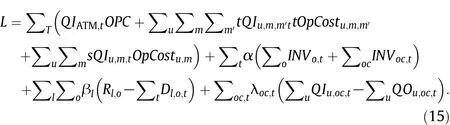
It can be separated as

and

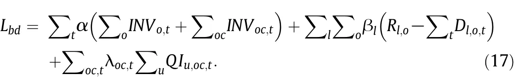
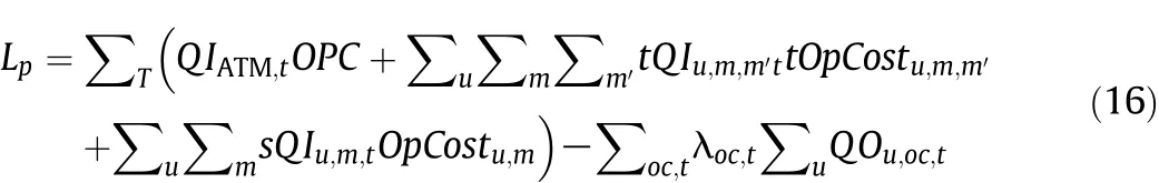
The production subproblem is denoted as P p and the blending and delivery subproblem is denoted as Pbd.

Pp:min Lp.

s.t.constraints(1)-(11),(13)and constraints(5)-(7)of Ref.[9]in model P0.

Pbd:min Lbd.

s.t.constraints(14)-(19),(21)-(28)of Ref.[9]in model P0.

The scheme of the Lagrangian decomposition algorithm is shown in Fig.2.The main challenges are initialization and update of Lagrange multipliers,solution method of subproblems and feasibility scheme of the primal problem.

3.2.Initialization and update of multipliers

In this paper,the mass balance constraints of component oils are relaxed and the scheduling problem is decomposed into two subproblems.The component oils can be considered as the products from the production stage and the raw material for the blending and delivery stage.The Lagrange multipliers can be considered as prices of the component oils.

For a given component oil oc,if the consuming amount in the blending and delivery part is larger than its production,that is,the value of Lagrangian multiplierλoc,twill increase in the updating step to increase the production of this component oil and decrease to use this component oil for blending.On the other hand,ifthe value ofλoc,twill decrease in the updating step.

Fig.2.Steps of the Lagrangian decomposition algorithm.

At proper prices,consumption∑uQIu,oc,tand production∑uQOu,oc,twill reach a balance.The Lagrange multipliers can be estimated by calculating the production costs of component oils.

where in Costuindicates the estimate cost of input material of unit u and out Costuindicates the estimate price of output product of unit u.

For a given unit u,the production cost of its output oil can be calculated as the sum of the cost of its inputoil and the operation costdivided by the yield of the output oil.Since unit u may have several operation modes,the operation cost and the yield are in the average sense.The estimated prices are taken as the initial Lagrange multipliers.

The subgradient optimization is a common method for updating a set of multipliers for the Lagrangian decomposition algorithm.In this paper,exponentially weighted subgradients[17]are used in the updating for faster convergence.The calculation formula is as follows.

where gi′t+1is the subgradient calculated from the solutions of subproblems,git+1is that used to update Lagrangian multipliers,and subscript it denotes the iteration.

3.3.Solving the subproblems

In the primal problem,there are no lower and upper bounds constraints for the component oils.The input amounts of component oils for blending are constrained by the mass balance constraint(14).The two subproblems are linear programming problems.When the blending and delivery subproblem is solved directly,the input of component oils for blending is 0 or its maximal values determined by the blending capacity,which are far away from the feasible solution of the primal problem.Thus the input amounts of component oils are constrained further by the yields of units from the production process.

Adding auxiliary constraint(20)to the blending and delivery subproblem will not influence the feasibility and optimality of the original problem.Besides,the blending and delivery subproblem can be solved more efficiently.

The new blending and delivery subproblem Pbd′is as follows:

Pbd′:min Lbd.

s.t.constraint(20)and constraints(14)-(19),(21)-(28)of Ref.[9]in model P0.

The efficiency of solving subproblems is critical in the Lagrange decomposition scheme.In this section,a speed-up algorithm is presented for solving the production subproblem.In the original problem,constraint(2)indicates an upper bound Nuof the total duration of transitions for unit u.When a smaller number nuis used to replace Nuin solving the production subproblem,it can be solved in less time with an approximate solution.When nuis updated to be close to Nuin the iterations,the solution of the production subproblem will be close to the accurate solution.

In the iterative algorithm,an increasing number nuis used to replace Nuin solving the production subproblem.And nuis updated according to the feasible solution.As the iteration goes on,nuwill reach its maximum.The updating rule of nuis as follows.

If nu＜,update nu=,whereis the duration of transitions for unit u from the feasible solution.

The production subproblem is reformulated as

Pp′:min Lp.

s.t.constraints(1),(2′),(3)-(11),(13)and constraints(5)-(7)of Ref.[9]in model P0.

3.4.Feasibility scheme

With the current value of Lagrange multipliers,the subproblems can be solved.Generally,the solutions of subproblems are not feasible for the primal problem by violating the dualized constraints.In this paper,it means that the production amount of a given component oil in the production subproblem is not equal to its consumption in the blending and delivery subproblem.Thus a feasibility scheme is needed.

With good Lagrange multipliers,the values of binary variables in the solutions of subproblems are close to the optimal values.Thus a heuristic algorithm is introduced to obtain solutions satisfying all constraints of the primal problem,including the mass balance constraints for component oils.In the heuristic algorithm,binary variables yu,m,tand xu,m,m′,tare fixed according to the solutions of subproblems,which can be described as constraints

where Uitdenotes the set of units with fixed binary variables fixed in iteration it.Each unit will be turned in some iterations.(yu,m,t)itand(xu,m,m′,t)itare obtained by the solutions of subproblems in iteration it.

Then,solve the feasible problem Pfeaas follows,the solution of which is a feasible solution of the original problem.

Pfea:min f.

s.t.constraints(1)-(13),(21)-(22)and constraints(5)-(7),

(14)-(19),(21)-(28)of Ref.[9]in model P0.

The solution of Pfeais a feasible solution of the original problem.

3.5.The stopping criteria

The stopping criteria of the Lagrangian decomposition algorithm are based on the dual gap and nuin the production subproblem.Criteria a and b should be both satisfied to stop the Lagrangian decomposition algorithm.

a:.gap≤ε.

b:nu=Nuor unchanged in k iterations.

Since the production subproblem is solved approximately,the dual objective value is not accurate.The current dual value is used to estimate the accurate one.The dual gap is calculated by the current dual value and the upper bound of the primal problem.

3.6.Complete Lagrangian decomposition algorithm

In summary,the Lagrangian decomposition algorithm is as follows.

Step 1:Decompose the reformulated model P into two subproblems Ppand Pbd.Reformulate Ppas Pp′and Pbdas Pbd′.

Step 2:De fine the feasible problem Pfea.

Step 3:Initialize the Lagrange multipliers by constraint(18).

Step 4:Solve subproblems and obtain the dual objective litby summarizing the objectives of the subproblems.

Step 5:Solve the feasible problem Pfea,calculate the objective of the original problem by the solution of Pfea,update the upper bound fupof the original problem P,and calculateu sing the solution of Pfea.If＞nu,set nu=

Step 6:If the stopping criteria are satisfied,stop the algorithm;otherwise,calculate the subgradient with constraint(19),update the Lagrange multipliers using constraint(23),and go to Step 4.

4.Case Study

In this section,three cases are used to test the proposed Lagrangian decomposition algorithm.The cases are solved by the reformulated model P and the Lagrangian decomposition algorithm separately.All the cases are executed by CPLEX 12.6.0.0 in GAMS 24.2.2 using a CPU Intel Xeon E5-2609 v2@2.5 GHz with RAM 32.0 GB.The scheduling horizons are discretized uniformly with time intervals of 8 h.The relative gap of the reformulated model P in CPLEX is set to 0.In the stopping criteria of the Lagrangian decomposition algorithm,the dual gap ε is set to 8%and k is set to 4.

The cases are based on the flow sheet in Fig.1.The sizes of the three cases are shown in Table 1.Case 1 and case 3 have the same number of orders,while case 2 and case 3 have the same number of time intervals.The key component concentration ranges of product oils are shown in Appendix B.The parameters of the scheduling model are shown in Appendix C.

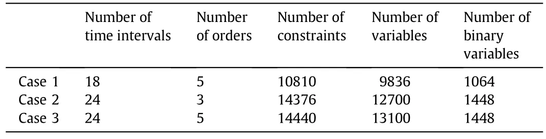
Table 1 Sizes of cases

4.1.Case 1

The orders of product oils for case 1 are given in Table 2.The statistics of solutions are shown in Table 3.Tl1and Tl2are the beginning time interval and due time interval for the delivery,respectively.

Table 2 Orders of product oils(time and quantity)for case 1

Table 3 The statistics of solutions for case 1

The iteration details of the Lagrangian decomposition algorithm are shown in Fig.3.The upper bound meets the optimal value of the primal problem at iteration 5.Compared with the upper bound,the convergence of the dual objective value is slower.The CPU time with the Lagrangian decomposition algorithm to meet the stopping criteria is about one third of that with the reformulated model P.

Fig.3.Convergence of the dual objective value and upper bound for case 1.

4.2.Case 2

The orders of product oils for case 2 are given in Table 4.The statistics of solutions are shown in Table 5.

Table 4 Orders of product oils(time and quantity)for case 2

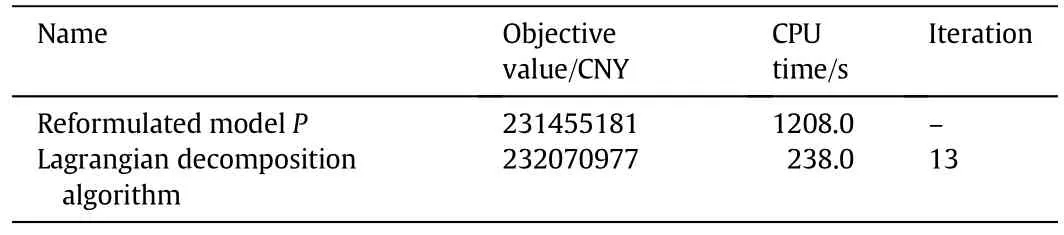
Table 5 The statistics of solutions for case 2

The iteration details of the Lagrangian decomposition algorithm are shown in Fig.4.The upper bound meets a near-optimal value of the primal problem atiteration 5.The gap between the near-optimal value and the optimal value is 0.27%.Compared with the upper bound,the convergence of the lower bound is slower.The CPU time with the Lagrangian decomposition algorithm is about one fifth of that with the reformulated model P.

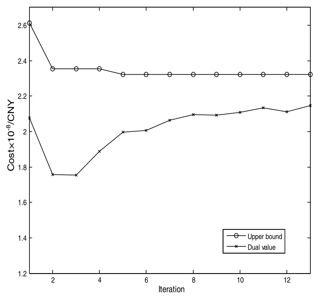
Fig.4.Convergence of the dual objective value and upper bound for case 2.

4.3.Case 3

The orders of product oils for case 3 are given in Table 6.The statistics of solutions are shown in Table 7.

The iteration details of the Lagrangian decomposition algorithm are shown in Fig.5.The upper bound meets the optimal value of the primalproblematiteration 5.Compared with the upper bound,the convergence of the lower bound is slower.The CPU time with the Lagrangian decomposition algorithm is about one tenth of that with the reformulated model P.

Table 6 Orders of product oils(time and quantity)for case 3

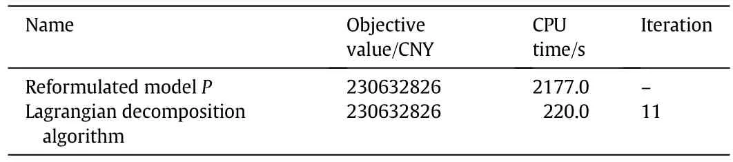
Table 7 The statistics of solutions for case 3

Fig.5.Convergence of the dual objective value and upper bound for case 3.

4.4.Summary

From the three cases,it is concluded that the Lagrangian decomposition algorithm can obtain the optimal or near-optimal solutions efficiently.The convergences of the dual objective values and upper bounds perform similarly on different scale cases.

The numbers of binary variables and constraints in case 2 are about 40%more than those in case 1.The number of binary variables in cases 2 and 3 is the same because the number of time intervals is the same,while the number of constraints in case 3 is a little more.Compared with case 1,case 3 has the same number of orders and more time intervals,so the numbers of binary variables and constraints in case 3 are about 40%more than those in case 1.It shows that as the scheduling time intervals increase,the primal problem usually leads to a very large scale combinatorial problem,which is difficult to solve.

The CPU time of the reformulated model P for case 2 is about 2.2 times that for case 1,while the CPU time with the Lagrangian decomposition algorithm for case 2 is about 29.3%more than that for case 1.The CPU time of the reformulated model P for case 3 is about 4 times of that for case 1,while the CPU time with the Lagrangian decomposition algorithm for case 3 is about 19.5%more than that for case 1.The solving time of the primal problem for case 3 is about 1.8 times that for case 2,while the CPU time with the Lagrangian decomposition algorithm decreases about 7.56%due to less iterations.

As the problem scale increases,especially the number of time intervals increases,the reformulated model P leads to a very large scale combinatorial problem and the advantage of the Lagrangian decomposition algorithm becomes more apparent.From Figs.3-5 we see that the dual objective value increases since iteration 3 and can infer that the accurate lower bound also increases.The optimalor near-optimal solutions are obtained in the early iterations,because the initial Lagrange multipliers are close to the optimal ones with the initialization step.The values of binary variables obtained by the solutions of subproblems are close to the optimalones.The stopping criterion of dual gap is set to 8%,which is sufficient for the algorithm to find the optimal or near-optimal solutions.

5.Conclusions

Short-term scheduling of refinery operations is one of the most challenging problems due to the complexity of production process.To reflect the dynamic nature of production,operation modes and transitions in mode switching are defined for each production unit.For large scale problems,the Lagrangian decomposition is a popular method,but the decomposition scheme depends on the problem structure.In this paper,the primal problem is decomposed to two subproblems by the mass balance constraints of component oils.Initial Lagrange multipliers are estimated and the solutions are close to the optimal one.Exponentially weighted subgradients are used in the updating for faster convergence.A speedup algorithm to increase the efficiency for solving the production subproblem and a heuristic algorithm to find feasible solutions are also designed.The computational results show that the Lagrangian decomposition algorithm is effective and efficient.The advantage of the proposed algorithm is especially apparent for large scale problems.

Nomenclature

Dl,o,tdelivery of product oil o for order l during time interval t

fupupper bound of original problem P

gitsubgradient for updating Lagrangian multipliers

git′subgradient calculated from the solutions of subproblems

INVo,tinventory of product oil o at the end of time interval t

INVoc,tinventory of component oil oc at the end of time interval t

inCostuestimate cost of input material of unit u

litdual objective at iteration it

Numaximum duration of transition for unit u in the primal problem

numaximum duration of transition for unit u in the production subproblem

OPC price of crude oil c

OpCostu,moperational cost of unit u in the operation mode m

outCostuestimate price of output product of unit u

QIu,oc,tinput amount of component oil oc from unit u during time interval t

QIu,oi,tinput amount of intermediate oil oi of unit u during time interval t

QIu,om,tin put amount of material oil om from unit u during time interval t

QOu,oc,toutput amount of component oil oc from unit u during time interval t

QOu,oi,toutput amount of intermediate oil oi of unit u during time interval t

QOu,om,toutput amount of material oil om from unit u during time interval t

QOu,s,toutput amount of port s of unit u during time interval t

Rl,odemand for product oil o of order l

sQIu,m,tinput amount of unit u during time interval t in the operation mode m

Tl1start time interval for delivery of order l

Tl2due time interval for delivery of order l

Tmaxmaximum number of time intervals in the scheduling horizon

tOpCostu,m,m′ operational cost of unit u in the transition from operation mode m to m′

tQIu,m,m′tinput amount of unit u during time interval t in the transition from operation mode m to m′

TTu,m,m′ time of the transition from operation mode m to m′of unit u

tYieldu,s,m,m′ yield of material leaving port s of unit u in the transition from operation mode m to m′

xu,m,m′,t1 for unit u in the transition from operation mode m to m′during time interval t

yu,m,t1 for unit u in the operation mode m during time interval t

Yieldu,s,myield of material leaving port s of unit u in the operation mode m

α inventory cost of component oils and product oils per period

βlpenalty for stock out of order l per ton

λoc,tLagrangian multiplier of component oil oc during time interval t

Subscripts

it iteration

l order of product oil

m operation mode

o product oils

oc component oils for blending

oi intermediate oils

om material oils

s unit port

t time intervals being scheduled

u production units

Appendix A

A.Yields and operation costs of processing units

Operation costs are given in kilograms of oil equivalent per ton;1 kgoe=41870 kJ.

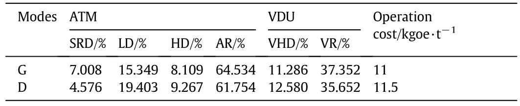
Table A1 Yields and operation costs of ATM and VDU

Table A2 Yields and Operation Costs of FCCU

Table A3 Yields and operation costs of HDS and ETH

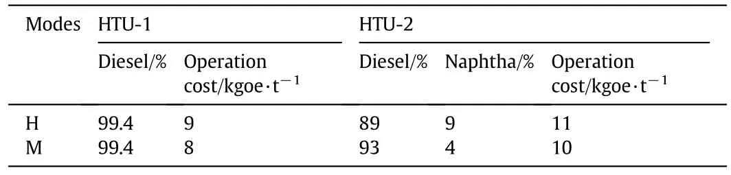
Table A4 Yields and operation costs of HTU-1 and HTU-2

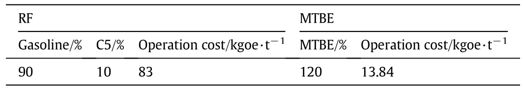
Table A5 Yields and operation costs of RF and MTBE

B.Key component concentration ranges of product oils

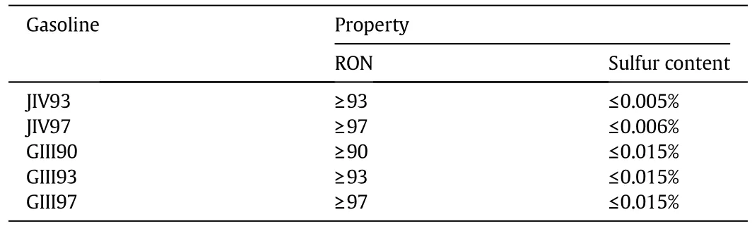
Table B1 Requirements for property value of gasoline

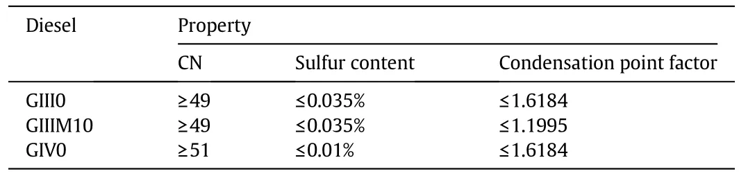
Table B2 Requirements for property value of diesel

C.Parameters of the scheduling model in case study section

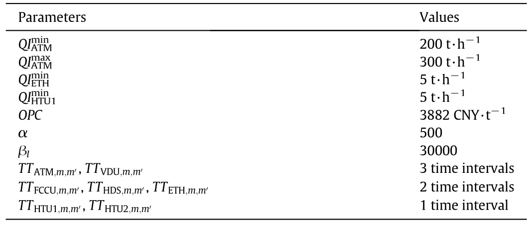
Table C1 Parameters of the scheduling model