A local and global statistics pattern analysis method and its application to process fault identification☆

Hanyuan Zhang,Xuemin Tian*,Xiaogang Deng,Lianfang Cai

College of Information and Control Engineering,China University of Petroleum(East China),Qingdao 266580,China

Keywords:Principal component analysis Local structure analysis Statistics pattern analysis Reconstruction-based contribution Fault diagnosis

ABSTRACT Traditional principal component analysis(PCA)is a second-order method and lacks the ability to provide higher order representations for data variables.Recently,a statistics pattern analysis(SPA)framework has been incorporated into PCA model to make full use of various statistics of data variables effectively.However,these methods omit the local information,which is also important for process monitoring and fault diagnosis.In this paper,a local and global statistics pattern analysis(LGSPA)method,which integrates SPA framework and locality preserving projections within the PCA,is proposed to utilize various statistics and preserve both local and global information in the observed data.For the purpose of fault detection,two monitoring indices are constructed based on the LGSPA model.In order to identify fault variables,an improved reconstruction based contribution(IRBC)plot based on LGSPA model is proposed to locate fault variables.The RBC of various statistics of original process variables to the monitoring indices is calculated with the proposed RBC method.Based on the calculated RBC of process variables' statistics,a new contribution of process variables is built to locate fault variables.The simulation results on a simple six-variable system and a continuous stirred tank reactor system demonstrate that the proposed fault diagnosis method can effectively detect fault and distinguish the fault variables from normal variables.

1.Introduction

Fault detection and identification are of ever growing importance for safe and efficient operations in complex industrial processes[1].With a large number of variables measured and stored automatically by distributed control systems,data-driven fault detection and identification based on the statistical process control theory have become one of the most fascinating topics in the process monitoring field.Notable algorithms based on principal component analysis(PCA)and partial least squares have been successfully applied to the detection of abnormal situations in industrial processes[2-4].However,the PCA-based methods lack the capability of providing higher-order representations for non-Gaussian data,which is the common case for industrial data,because PCA is a second-order method and only considers the mean and variance-covariance of the data.

To utilize different statistics information hidden in original measured variables,several multivariate monitoring methods based on higher-order statistics information have been proposed.Independent component analysis is used to extract several components that are statistically independent and non-Gaussian distributed from process data[5,6].As an emerging technique based on a new multivariate statistical process monitoring framework,statistics pattern analysis(SPA)[7,8]is proposed and it is of superiority over PCA for industrial process monitoring.It is argued that the statistics of variables follow Gaussian distribution,in spite of the non-Gaussian distribution of the original variables.Furthermore,these statistics capture different characteristics of process data,and the statistics under abnormal conditions would show important discrimination information for fault diagnosis.Although fault detection methods derived based on the SPA framework have been successfully employed to detect process faults,the faultidentification with SPA framework has rarely been studied except for[9,10].Traditional contribution plots for fault identification are constructed from SPA framework[9]and SPA similarity factor method is proposed to identify faults[10].However,the SPA-based fault diagnosis methods only capture the global structure information and ignore detailed local structure information during process monitoring.

The local structure information of process data is an important aspect of the dataset for data mining and feature extraction,since it represents detailed relationship between different data samples[11].The loss of this information may have adverse impact on dimension reduction performance.Recently,locality preserving projection(LPP)is proposed to optimally preserve the intrinsic geometry structure of the data in a low-dimensional space[12]and it has been successfully applied to the fault detection in industrial processes[13-15].To well consider both local and global data information during dimensionality reduction,Zhang et al.[16]proposed a global-local structure analysis model which combines the advantage of PCA and LPP under a unified framework.Other dimension reduction methods based on local and global structure analysis,such as LGPCA and LKPCA[17,18],have been proposed for fault detection.

After a fault is detected,the fault variables need to be isolated in order to diagnose the root causes of the fault.One popular approach is to use contribution plots to identify the variables pushing the monitoring indices out of their control limits[19,20]and does not need prior fault information and is easy to use.Contribution plots are based on the idea that variables with large contributions to a fault detection index are likely the cause of the fault.Although contribution plots have found wide applications in various processes,they fail to guarantee correct diagnosis due to the smearing effect,even for simple sensor faults[21].

As an alternative method to determine the root cause of a fault,the reconstruction can be employed.Dunia and Qin[22]proposed a reconstruction-based method to characterize faults by fault directions and used the fault direction information to perform fault identification via reconstruction.By incorporating T2and SPE indices,Yue and Qin[23]developed a combined index to identify faults based on the reconstruction-based method.These reconstruction-based methods can guarantee correct diagnosis when the fault directions are known and are in the candidate set of directions,but they cannot guarantee identification accuracy for faults with unknown directions.To make an improvement,Alcala and Qin[21]proposed a reconstruction-based contribution(RBC)with PCA model to find sensor fault directions and amplitudes that,if removed,would minimize associated fault detection index value.This method inherits the merit of traditional contribution plots and has a solid theoretical foundation for sensor faults.The RBC has been extended from linear case to nonlinear case in[24].

According to the above analysis,this paper develops a local and global statistics pattern analysis(LGSPA)method for fault diagnosis by integrating both SPA framework and LPP into a PCA model.SPA is utilized to calculate various statistics of process variables to substitute for the original variables and LPP is used to consider local data information during dimension reduction.Two monitoring indices are built based on the proposed LGSPA model for fault detection.After a fault is detected,an improved RBC is proposed to address the important issue of fault identification.The RBC of various statistics of original process variables is derived from the fault detection indices generated by LGSPA model.Then,a new RBC of a variable is defined for fault identification based on the RBC of variables' statistics.The major difference between traditional RBC method and the proposed RBC method is that the former is constructed based on process variables while the latter is based on various statistics of original process variables.In addition,we extend the relative contribution[25]to the proposed RBC method to obtain much clearer indication.Simulations on a simple six-variable system and a continuous stirred tank reactor(CSTR)process are used to demonstrate the superiority of the proposed fault diagnosis scheme.

2.Basic Theory

2.1.Principal component analysis

PCAcan easily handle high dimensional,noisy,and highly correlated data by projecting the original data to a lower-dimensional subspace that contains the most variance of original data and accounts for correlations among different variables[1,3].In addition,PCA only requires easily available normal operation data to develop the normal operating condition model[18].Due to these advantages,PCA-based monitoring methods have been widely studied.

Let X=[x1,x2,…,xn]T∈ Rn×mbe normal process data,which represents m columns of measured variables at n rows of sample points,PCA decomposes the data matrix X as

where ti∈Rn×1is the i-th score vector,pi∈Rm×1is the i-th loading vector,l is the number of principal components(PCs)in the PC model,and E is the residual matrix.The loading vector pirepresents the i-th principal direction in the PC subspace,which corresponds to the i-th eigenvector of the covariance matrix

where λi′is the eigenvalue corresponding to eigenvector pi,X is to be scaled by subtracting the mean of the normal operation dataset and dividing each column by the standard deviation of normal operation dataset.The monitoring index SPE is defined as a measure of the variations in the residual subspace

where x ϵ Rm×1is a column vector with m variables,^x=PPTx and~C′=Im-PPT,Imϵ Rm×mis the identity matrix.P=[p1,p2,…,pl]is the loading matrix.The control limit 100(1- α)%of the SPE index is σ2=with g=,h=andwhich is proposed by Nomikos and MacGregor[26].

T2is another fault detection index to measure the variations in the PC subspace:

where D′=PΛ′-1PTand Λ′is the diagonal matrix with the variances of PCs as the diagonal elements.

The 100(1- α)%upper control limit τ2for T2statistic can be obtained using the F-distribution[27]:

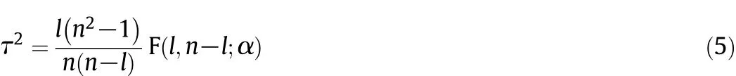
where F(l,n-l;α)is an F-distribution with l and n-l degrees of freedom,and a significance level α.

2.2.Traditional reconstruction-based contribution

When a fault is detected by any one of the above-mentioned fault detection indices,an identification tool is required to determine fault variables.Contribution plots are very popular for fault identification,which do not require specific fault information[19,20].However,contribution plots may cause misleading identification result when some faults involve many related fault variables[22].In order to overcome this shortcoming of traditional contribution plots,Alcala and Qin proposed a reconstruction-based contribution(RBC)method to identify fault variables[21].This method analyzes the variable contribution based on the reconstruction of the fault detection index along the directions of variables,which improves identification results.The traditional RBC of variable xito a fault detection index is defined as:

where Γ represents a specific matrix defined by the fault detection index,Γ =~C′for SPE and Γ =D′for T2,Γiiis the i-th diagonal element of Γ,and ξiis the i-th column of identity matrix and the direction of xi.

3.Local and Global Statistics Pattern Analysis

For the purpose of diagnosing fault effectively,the LGSPA method is proposed not only to utilize various statistics of original process variables but also to preserve both local and global structure information of observation dataset in dimension reduction.In the proposed LGSPA method,the SPA framework is first used to characterize the process behavior by statistics of process variables(i.e.,statistics pattern),instead of by process variables themselves.After the statistics patterns(SPs)[7,8]are obtained from normal and faulty datasets,the method[16]is applied to reduce the dimension through considering both global and local structure analysis of the SPs.

For the data matrix X=[x1,x2,…,xn]T∈Rn×mmeasured under the normal operating condition,we use Xkto denote a window of process measurements

where w is the window width and k is the current time index.

Statistics pattern(SP)[7,8]consists of three kinds of process statistics: first-order,second-order and higher-order statistics.The firstorder statistics are means,expressed as

The second-order statistics are variances,expressed as

The higher-order statistics include the third-order statistics,skewness(γi)and the fourth-order statistics,kurtosis(κi).They measure the extent of nonlinearity and quantify the non-Gaussianity of process variables.Specially,skewness and kurtosis measure the asymmetry and peakedness of process variables' distributions respectively.

In this paper,we use the four statistics ui,vi,γiand κi.After they are computed,a SP is obtained by stacking them into a row vector,and the SPs from different windows are used to build the training matrix.

where J(a)Globalis used to preserve the global structure of the dataset,and the local structure is preserved with J(a)Local.Parameter η is introduced to balance the two objectives,which can be changed with process datasets.a ∈ Rmsp×1is the projection vector and Q ∈Rmsp×mspis defined as

The solution of function(12)can be obtained by solving the eigenvalue decomposition

Suppose a1,a2,…,adare the obtained eigenvectors of Q corresponding to the first d maximum eigenvalues λ1,λ2,…,λd.The LGSPA loading matrix A can be written as A= ［a1,a2,…,ad］∈ Rmsp×d.Denote Λ =diag(λ1,λ2,…,λd),where diag()denotes the d × d diagonal matrix.Note that the projection vectors calculated from LGSPA are mutually orthogonal.The advantage of the orthogonal vectors is that it can effectively enhance the discriminating ability of dimension reduction methods,which is desirable for fault identification.

Matrix Xspis decomposed into feature space and residual space.

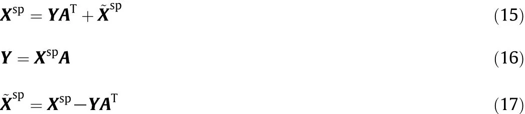
where Y ∈ Rnsp×dis the score matrix and the score vectors are also mutually orthogonal,and~Xsp∈Rnsp×mspis the residual matrix.

When a single measurement or a block of new measurements is available,the window shifts forward by one or multiple samples and a new SP∈ Rmsp×1is computed.It can be projected in the feature space and residual space.

where ynew=is a vector of the scores and∈ Rmsp×mspis the identity matrix.

Let Dpand Drdenote T2and SPE in the LGSPA,respectively.The monitoring index Dpis built to measure the dominating variation in feature space,defined as

where D=AΛ-1AT.

The monitoring index Drindicates how wellthe current SP conforms to the model

After monitoring indices Dpand Drare obtained,proper control limits for them must be defined to determine whether the process is operated under normal condition.In our work,the well-known kernel density estimation method[28]is used to determine the confidence limits.If any monitoring index exceeds its confidence limit,an abnormal behavior of the process is detected.

4.The Improved RBC Plots with LGSPA Model

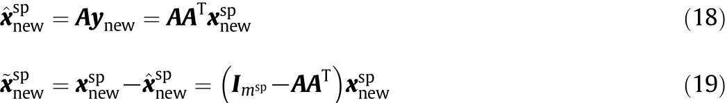
Once a fault is detected by monitoring indices,it is the task of fault identification to identify fault variables and to locate root cases,which is a challenge in fault diagnosis.Inspired by[21],we present an improved RBC method to identify fault variables using the LGSPA model.The amount of reconstruction along a statistic direction in the SP that minimizes the fault detection index is defined as the LGSPA-based RBC of that statistic.A new RBC of a variable to the fault detection index is defined as the sum of the RBC of statistics(i.e.,mean,variance,skewness and kurtosis).Forcalculated from the fault measurements,the reconstructed vector zsp,ialong the fault direction ξiof the i-th statistic is calculated as

Here,ξi= ［0,,,0,…,1,…,0］T∈ Rmsp×1is the column of the identify matrix and fiis the fault magnitude along ξi.

The objective of LGSPA-based RBC is to find a value of fito minimize the fault detection index of the reconstructed measurement.

where M=D for Dpindex and M=~C for Drindex.

This minimization is done by taking the first derivative ofIndex(zsp,i)with respect to fiand setting it to 0.

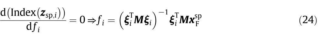
The reconstruction-based contribution of the i-th statistic in the SP to the fault detection index is the amount of reconstruction along the direction ξi.

Substituting Eq.(24)into Eq.(25),we obtain

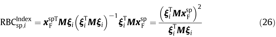
Specially,the RBC of the i-th statistic to Dris obtained using M=~C.

The RBC of the i-th statistic to Dpcan be found by setting M=D in Eq.(26).

where diiis the i-th diagonal element of D.

In order to achieve more accurate fault identification,we adopt the relative contribution value of each statistic in the SP with respect to some normaloperating condition[18,25].More specifically,letdenote the RBC value of the i-th statistic in a SP under the normal operation condition,mean(·)and std(·)denote mean and standard deviation operators,which are performed over the whole training dataset Xsp.Then,the relative RBC(RRBC)value of the i-th statistic in a SP to the fault detection index is given by

Usually,the sign of relative RBC is not important and the absolute value indicates the effect of process variable statistics to its corresponding index.Thus the absolute value of relative RBC is used in this paper.

According to the literature[7],the mean,variance,skewness and kurtosis statistics under abnormal conditions would deviate from the distribution of these statistics under normal operation,because the above four statistics capture different characteristics of the process.Therefore,when a fault occurs,the RBCs of the four statistics of the fault variable would respond to the fault and would be much larger than the RBCs of the corresponding statistics of other variables'.On the basis of the aforementioned analysis,an improved RBC(IRBC)of the i-th variable to a fault detection index is proposed.

These relative RBCs of are first scaled with their own standard deviation before Eq.(30)is used.A large value ofindicates that the i-th variable is likely the root cause of faults.In addition,the value ofcalculated using one SP is always influenced by many uncertainties,such as measurement noise.Therefore we use the average contribution over several fault SPs to provide a more stable conclusion.

A complete application procedure of the proposed fault identification method includes off-line modeling and on-line identification stages.In the off-line modeling stage,the normal operating model is developed by the LGSPA method.In the on-line identification stage,after a fault is detected,fault SP is generated from the fault data and improved RBC plots of the variables are calculated to determine which variable is responsible for the fault.The detailed fault identification procedure can be summarized as follows.

4.1.The off-line modeling stage

(1)Compute various statistics of the process variables using the moving window technology based on dataset X acquired from normal operation condition.

(2)Stack all statistics into a row vector to obtain a SP and put the SPs calculated from different windows together to build training matrix Xsp.

(3)Normalize training matrix Xspwith the mean and variance of each statistic.

(4)Construct matrix Q according to Eq.(13)and solve the eigenvalue problem in Eq.(14)to obtain the first d maximumeigen values and their corresponding d eigenvectors.

4.2.The on-line identification stage

(1)Compute the fault statistics patternfrom a window of fault dataset.

(3)Compute the RBC of the statistics into fault monitoring indices Drand Dpaccording to Eqs.(27)and(28),respectively.

(4)Calculate the relative contribution of each statistic based on Eq.(29)and compute the improved RBC of the variables according to Eq.(30).

(5)Compare the values of the improved RBC of process variables and the variable with the largest improved RBC is recognized as the fault variable.

In order to compare the fault identification performance between traditional RBC method and the proposed RBC method,the concepts of relative contribution and average contribution are also applied to the traditional RBC method.Furthermore,two performance indices are defined in this work for evaluating the fault identification performance.One index is called identified variable index(IVI),defined as

which represents the index of the variable with the largest RBC to the fault detection index.

Another performance index is to judge the contrast degree by comparing the largest and the second largest RBC,and,of the variables to the fault detection index,called as identification contrast degree(ICD)and expressed as

Low contrast degree refers to a convincing,clear and correct identification.

5.Simulation Study

This section compares the proposed fault diagnosis method with the traditional PCA-based method by two case studies:a simple six-variable system and a CSTR process.

5.1.A simple six-variable system

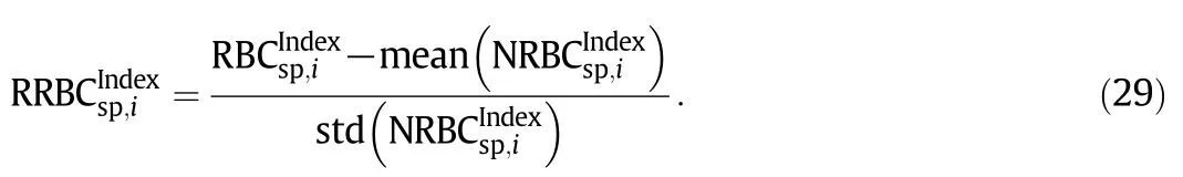
In this section,a simple system with six monitored variables is simulated to test the faultidentification performance of the proposed method.This system is a modified version of the system studied by Ge et al.[29],whose mathematical description is given as

The mixing matrix A is randomly selected:

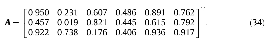
The three independent components s=[s1,s2,s3]Tare uncorrelated source signals,each of which follows a uniform distribution within[0,1],and e are Gaussian distributed with the means as 0 and variances as 0.01.Normal dataset with 1000 samples are simulated as reference dataset.Two faults in Table 1 are simulated to generate fault datasets with 1000 samples and for each fault dataset,fault is introduced at the 250-th sample.

Conventional PCA method and the proposed LGSPA methods are first used for fault detection and their performance is compared.In the PCA-based method,the number of principal components is selected as 3 so that the eigenvalue cumulative is above 95%of the sum of all the eigenvalues.The alarm threshold is set to the 99%confidence limit.Because three principal components are retained in the PCA model,the same number of vectors generated by the LGSPA model is also selected for comparison.In the LGSPA-based method,the 99%confidence limits for monitoring indices Dpand Drare calculated.As the LGSPA is a window-based approach,the window width w is a crucial parameter.However,in the present study on statistics pattern analysis[7,8],no conclusion has been given about how to determine this parameter.Parameter w is set to be 40 by experiment testing and each time the window is shifted by 10 samples.Consequently,the faults are equivalent to be introduced at the 22-nd SP.The number of the nearest neighbors is set as kN=10 and parameter η is set to be 0.5.After a fault is detected,it is important to identify the process variables that cause the fault.In our work,the PCA-based RBC method and LGSPA-based RBC method are applied to identify fault variables for performance comparison.

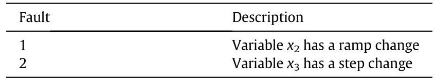
Table 1 Description of the two faults

Fault 1 is a ramp change in variable x2.The PCA-based monitoring charts in Fig.1 indicate that T2statistic detects this fault at the 346-th sample and SPE statistic detects it at the 353-rd sample.When the proposed LGSPA method is applied,Fig.2 shows that this fault is detected by Dpstatistic at the 23-rd SP and by Drstatistic at the 27-th SP.In further analysis,two methods have different fault alarming rates.Fault alarming rates of T2and SPE statistics in the PCA-based fault detection method are 87.20%and 86.27%,respectively,while LGSPA-based fault detection method performs better,Dpand Drstatistics achieve the fault alarming rates as 97.33%and 93.33%,respectively.

Next,fault identification results of the two methods are shown in Figs.3 and 4,respectively.For the PCA-based RBC,the contribution value is calculated as the average contribution of the 30 samples right after the 346-th sample and that of the LGSPA-based RBC is calculated as the average contribution of the 3 SPs right after the 32-nd SP.As shown in Fig.3,the traditional RBC to T2and SPE both indicate that variable 2 has the largest contribution to this fault,while RBCs of other variables are also very large,especially that of variables for SPE statistic,which would lead to an unconvincing conclusion.In contrast,the proposed RBC plots shown in Fig.4 not only identify the root cause of the fault correctly but also have a large difference between the RBC value of fault variable and those of normal variables,which ensures the clear identification with high contrast degree.

A summarized comparison of the two RBC methods is given by performance indices in Table 2.Although both PCA-based RBC and LGSPA-based RBC methods can determine the root cases of faults 1 and 2 correctly,their identification contrast degrees are quite different.The values of ICD to T2and SPE indices for the two faults are all above 0.5 and the largest value is 0.957,indicating that the performance of traditional RBC method is not satisfactory because it has large identification contrast degrees.On the contrary,the proposed RBC method gives ideal results because the values of ICD to Dpand Drindices are all blew 0.3 and the smallest value is 0.1147.

5.2.A continuous stirred tank reactor

The proposed fault identification strategy is tested with a nonisothermal CSTR with feedback control systems[6,30],which is shown in Fig.5.It is assumed that a classic first order irreversible reaction occurs in the CSTR.The flow of solvent and reactant A into a reactor produces a single component B as an outlet stream.Heat from the exothermic reaction is removed through the cooling flow of jacket.The temperature of reactor is controlled by manipulating the coolant flow and the level is controlled by manipulating the outlet flow.

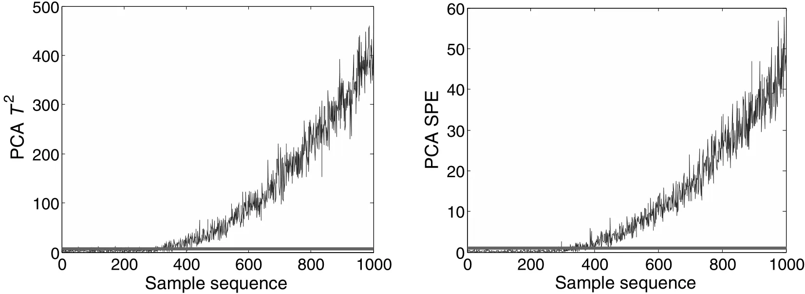
Fig.1.Monitoring charts of the PCA for Fault 1.

Fig.2.Monitoring charts of the LGSPA for Fault 1.

Fig.3.Fault identification using the PCA-based RBC plots for Fault 1.

The data of normaloperating condition and fault conditions are generated by simulating the CSTR process.Ten process variables listed in Table 3 are recorded and non-Gaussian noise is added to all process variables to obtain non-Gaussian data in simulation procedure.The fault patterns are given in Table 4.In the simulation,data are sampled every 2 s and 900 samples are stored.For each fault pattern,fault is introduced at the 201-st sample.

The PCA-based method and the LGSPA-based method are used to detect fault.In the PCA method,eight principal components are preserved,which capture about 95%of the variance of process data.The alarm threshold is set to the 99%confidence limit.For comparison,the number of the latent variables for the LGSPA model is also selected as 8 and the 99%confidence limit of each monitoring index is determined as the alarm threshold.The parameter w is set to be 40 in the simulation and each time the window is shifted by 10 samples.The faults are equivalent to be introduced at the 17-th SP.Parameter η is set to be 0.5 and kNis chosen as 10.After a fault is detected,the two methods are applied to identify fault variables.

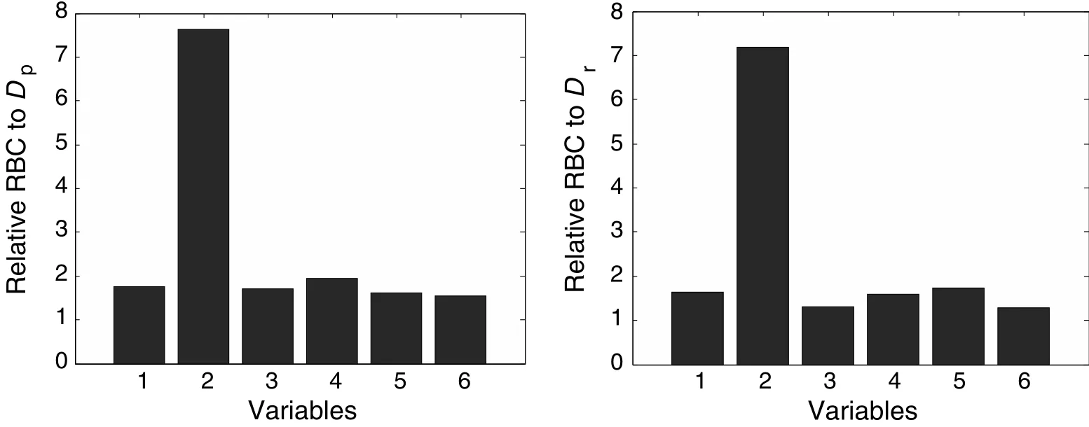
Fig.4.Fault identification using LGSPA-based RBC plots for Fault 1.

Table 2 Identification performance index for two faults

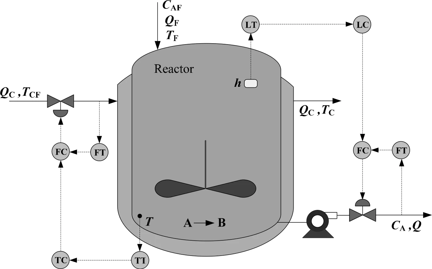
Fig.5.A diagram of the CSTR system.

Fault F1 is the step change in feed flow rate(variable 5).The monitoring results of PCA and LGSPA for Fault F1 are shown in Figs.6 and 7,respectively.Fig.6 indicates that both T2and SPE indices detect this fault at the 201-st sample.Two monitoring charts of LGSPA in Fig.7 indicate the fault quickly at the 17-th window.

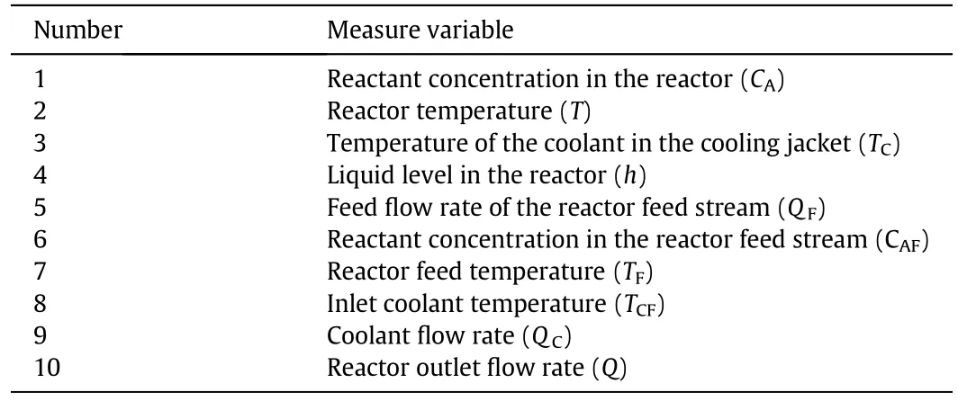
Table 3 Monitoring variables in CSTR process

For the PCA-based RBC method,the contribution value is calculated as the average value from the 201-st sample to the 231-st sample.For the LGSPA-based RBC,the contribution value is calculated as the average value from the 17-th SP to the 20-th SP.The PCA-based T2and SPE RBC plots are illustrated in Fig.8 and the LGSPA-based Dpand DrRBC plots are illustrated in Fig.9.Fig.8 indicates that RBC plot for T2is more apparent to identify the fault variable(i.e.,variable 5)while RBCplot for SPE still cannot give the accurate fault variable.For the LGSPA-based RBC method,the RBC plots for both indices Dpand Drindicate variable 5 as the maximum contributor to the fault,which is much clearer than the PCA-based RBC method.

Table 4 Fault patterns of CSTR system

Fig.6.The monitoring charts of the PCA for Fault F1.

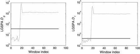
Fig.7.The monitoring charts of the LGSPA for Fault F1.

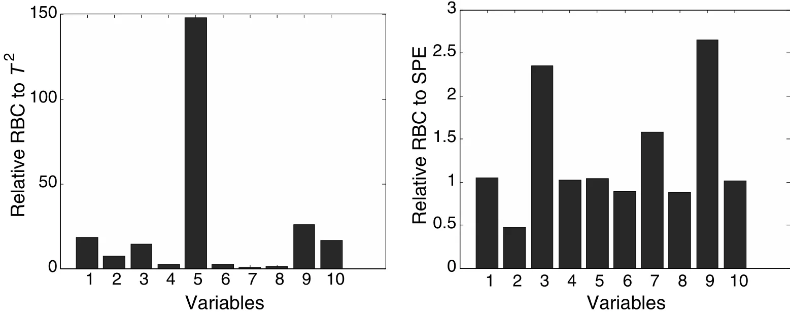
Fig.8.Fault identification using the PCA-based RBC plots for Fault F1.

The fault detection results of the PCA and the LGSPA for Fault F3 are shown in Figs.10 and 11.Fault F3 involves the ramp variation of feed temperature(variable 7),it is detected by the T2index at the 269-th sample,while the SPE index performs worse and gives alarming signal at the 432-nd sample.By contrast,LGSPA improves the monitoring performance and its statistics Dpand Drdetect the fault at the 20-th and the 18-th windows,respectively.In further analysis,the fault detection rates of statistics T2and SPE in the PCA-based fault detection method are 90.14%and 66.86%,respectively,while the fault detection rates of statistics Dpand Drin LGPCA-based fault detection method are 95.71%and 98.57%,respectively.

After the fault sample detected by T2,30 samples are used to calculate the average contribution for the PCA-based RBC plots,illustrated in Fig.12,and the LGSPA-based RBC plots using the average contribution from the 24-th SP to the 27-th SPare illustrated in Fig.13.With the PCA-based RBC method,variable 7 is identified as the root cause of the fault by the RBCplotfor T2.While the RBC plot for SPE suggests that variable 5 is affected most,which is an incorrect analysis.With the LGSPA-based RBC method,we can find that the largest contribution to indices Dpand Dris from variable 7.The results in Fig.13 indicate the proposed RBC method can find abnormal variables more clearly and more accurately than the traditional RBC method.

Fig.9.Fault identification using the LGSPA-based RBC plots for Fault F1.

Fig.10.The monitoring charts of the PCA for Fault F3.

Fig.11.The monitoring charts of the LGSPA for Fault 3.

After the five faults(F1-F5)are detected,the next step is to identify fault variables.Two kinds of RBC for the five faults are calculated and the quantitative performance comparison is executed by indices IVI and ICD,listed in Table 5.When traditional RBC or improved RBC to a fault detection index cannot identify the fault variable correctly,there is no need to further calculate its ICD.The results show that the traditional RBC for indices T2and SPE is unable to identify the faulty variables clearly for the five faults,since the values of ICD for faults F2,F4 and F5 are all above 0.8.In contrast,the proposed RBC for both indices Dpand Drcan find the true fault variables for all of the five faults with the values of ICD are all blew 0.5,which means clear identification.According to the above results and analysis,the proposed RBC method is superior to the traditional RBC method in terms of recognizing fault variables.

6.Conclusions

In the present paper,a new process monitoring method,referred to as the LGSPA,is proposed.The SPA frame work is extended to PCA model to mine the information of the statistics of process variables.In addition,the local structure analysis is integrated into the global optimization of the PCA technique naturally.After a fault is detected,an improved RBC method based on LGSPA model is developed to identify fault variables.The improved RBC is constructed based on various statistics of original process variables while the traditional RBC is calculated based on original process variables.Simulations on a simple six-variable system and a CSTR process demonstrate that the proposed fault diagnosis strategy can effectively detect process fault and distinguish the fault variables from the normal variables.

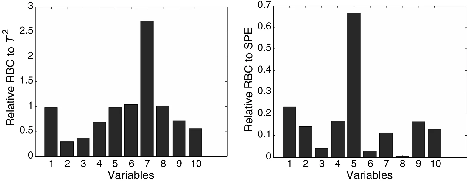
Fig.12.Fault identification using the PCA-based RBC plots for Fault F3.

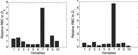
Fig.13.Fault identification using LGSPA-based RBC plots for Fault F3.

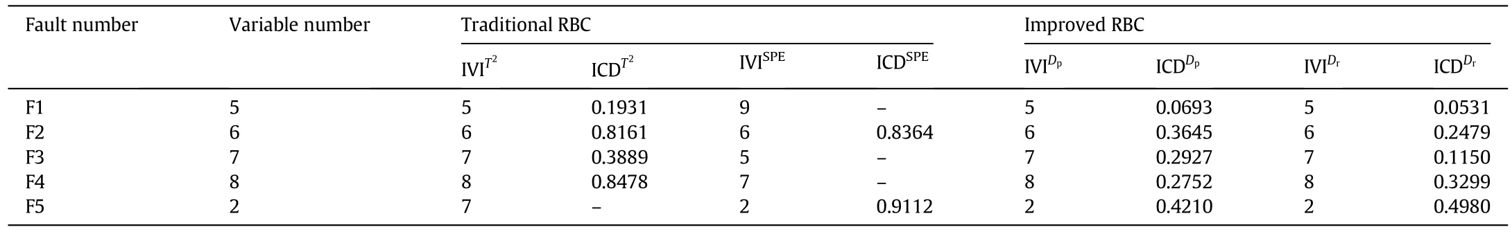
Table 5 Identification performance index for five faults

However,several open issues deserve to be further studied.One is the mechanism how the window width and window overlapping affect the fault diagnosis performance.Another is to enhance the fault identification performance by applying the weighting strategy to different statistics.Our future research will focus on these two points.

Nomenclature

A loading matrix of LGSPA

a loading vector of LGSPA

D covariance matrix of loading matrix of LGSPA

D′ covariance matrix of loading matrix of PCA

Dpmonitoring index of LGSPA in principal component space

Drmonitoring index of PCA in residual space

d number of loading vector retained in LGSPA

diii-th diagonal element of D

E residual matrix of PCA

fifault magnitude along direction of the i-th statistic

H diagonal matrix whose entries are column sums of proximity matrix

Imthe m×m identity matrix

Imspthe msp×mspidentity matrix

ICDIndexcontrast degree of the largest and the second largest RBC of variables to a fault detection index

Index(zsp,i)fault detection index of reconstructed measurement

IRBCIindeximproved RBC of the i-th variable to a fault detection index

IVIIndexindex of the variable with the largest RBC to a fault detection index

J(a)LGSPAobjective function of LGSPA

k current time index

kNnumber of the nearest neighbors in the LGSPA

l number of principal components retained in the PCA model

m number of measured variables

mspnumber of statistics in one SPs

NRBCIsnpd,iexRBC of the i-th statistic under normal operation condition to a fault detection index

n number of sample points

nspnumber of statistics patterns

P loading matrix of PCA

pii-th loading vector of PCA

RBCIindextraditional RBC of variable xito a fault detection index

RBCDspp,iRBC of the i-th statistic to Dp

RBCDspr,iRBC of the i-th statistic to Dr

RRBCIsnpd,iexrelative RBC value to a fault detection index

S proximity matrix

SPE monitoring index of PCA in residual space

T2monitoring index of PCA in principal component space

tii-th score vector of PCA

uimean of the i-th variable

vivariance of the i-th variable

w window width

X normal operating dataset

Xkwindow of process measurements

Xspstatistics pattern matrix under normal operating condition

x measurement vector

^x projection of measurement vector to the principal component subspace

xsipi-th statistics pattern

xsnpewstatistics pattern of testing sample

xii-th original variable

Y score matrix of LGSPA

ynewvector of the scores of LGSPA

zsp,ireconstructed vector along direction of the i-th statistic

Γ specific matrix defined by fault detection index

Γiii-th diagonal element of Γ

α confidence coefficient

γiskewness of the i-th variable

η trade-off parameter in LGSPA

κikurtosis of the i-th variable

Λ diagonal matrix whose diagonal elements are the d maximum eigenvalue of LGSPA

Λ′ diagonal matrix whose diagonal elements are the variances of PCs in PCA

λii-th eigenvalue of LGSPA

λi′ i-th eigenvalue of PCA

ξii-th column of identity matrix

σ2control limit of the SPE index

τ2upper control limit of T2