
Nuclear charge radius predictions by kernel ridge regression with odd-even effects
2024-04-25 07:14LuTangZhenHuaZhang
Nuclear Science and Techniques 2024年2期
Lu Tang · Zhen-Hua Zhang,2
Abstract The extended kernel ridge regression (EKRR) method with odd—even effects was adopted to improve the description of the nuclear charge radius using five commonly used nuclear models.These are: (i) the isospin-dependent A1∕3 formula, (ii)relativistic continuum Hartree—Bogoliubov (RCHB) theory, (iii) Hartree—Fock—Bogoliubov (HFB) model HFB25, (iv) the Weizsäcker—Skyrme (WS) model WS* , and (v) HFB25* model.In the last two models, the charge radii were calculated using a five-parameter formula with the nuclear shell corrections and deformations obtained from the WS and HFB25 models,respectively.For each model, the resultant root-mean-square deviation for the 1014 nuclei with proton number Z ≥8 can be significantly reduced to 0.009-0.013 fm after considering the modification with the EKRR method.The best among them was the RCHB model, with a root-mean-square deviation of 0.0092 fm.The extrapolation abilities of the KRR and EKRR methods for the neutron-rich region were examined, and it was found that after considering the odd—even effects,the extrapolation power was improved compared with that of the original KRR method.The strong odd—even staggering of nuclear charge radii of Ca and Cu isotopes and the abrupt kinks across the neutron N =126 and 82 shell closures were also calculated and could be reproduced quite well by calculations using the EKRR method.
Keywords Nuclear charge radius · Machine learning · Kernel ridge regression method
1 Introduction
The nuclear charge radius, similar to other quantities such as the binding energy and half-life, is one of the most basic properties reflecting the important characteristics of atomic nuclei.Assuming a constant saturation density inside the nucleus, the nuclear charge radius is usually described by theA1∕3law, whereAis the mass number.By studying the charge radius, information on the nuclear shells and subshell structures [1, 2], shape transitions [3, 4], the neutron skin and halos [5—7], etc., can be obtained.
With improvements in the experimental techniques and measurement methods, various approaches have been adopted for measuring the nuclear charge radii [8, 9].To date, more than 1000 nuclear charge radii have been measured [10, 11].Recently, the charge radii of several very exotic nuclei have attracted interest, especially the strong odd—even staggering (OES) in some isotope chains and the abrupt kinks across neutron shell closures [2, 12—21], which provide a benchmark for nuclear models.
Theoretically, except for phenomenological formulae[22—29], various methods, including local-relationship-based models [30—35], macroscopic—microscopic models [36—39],nonrelativistic [40—43] and relativistic mean-field model[44—52], were used to systematically investigate nuclear charge radii.In addition, theabinitio no-core shell model was adopted for investigating this topic [53, 54].Each model provides fairly good descriptions of the nuclear charge radii across the nuclear chart.However, with the exception of models based on local relationships, all of these methods have rootmean-square (RMS) deviations larger than 0.02 fm.It should be noted that few of these models can reproduce strong OES and abrupt kinks across the neutron shell closure.To understand these nuclear phenomena, a more accurate description of nuclear charge radii is required.
Recently, due to the development of high-performance computing, machine learning methods have been widely adopted for investigating various aspects of nuclear physics[55—59].Several machine learning methods have been used to improve the description of nuclear charge radii, such as artificial neural networks [60—63], Bayesian neural networks[64—68], the radial basis function approach [69], the kernel ridge regression (KRR) [70], etc.By training a machine learning network using radius residuals, that is, the deviations between the experimental and calculated nuclear charge radii, machine learning methods can reduce the corresponding RMS deviations to 0.01-0.02 fm.
The KRR method is one of the most popular machinelearning approaches, with the extension of ridge regression for nonlinearity [71, 72].It was improved by including odd—even effects and gradient kernel functions and provided successful descriptions of various aspects of nuclear physics, such as the nuclear mass [73—77], nuclear energy density functionals [78],and neutron-capture reaction cross sections [79].In the present study, the extended KRR (EKRR) method with odd—even effects included through remodulation of the KRR kernel function [74] was used to improve the description of the nuclear charge radius.Compared with the KRR method, the number of weight parameters did not increase in the EKRR method.
The remainder of this paper is organized as follows.A brief introduction to the EKRR method is presented in Sect.2.The numerical details of the study are presented in Sect.3.The results obtained using the KRR and EKRR methods are presented in Sect.4.The extrapolation power of the EKRR method was discussed.The strong OES of the nuclear charge radii in Ca and Cu isotopes and abrupt kinks across the neutronsN=126 and 82 shell closures were investigated.Finally,a summary is presented in Sect.5.
2 Theoretical framework

wherexiare the locations of the nuclei in the nuclear chart,withxi=(Zi,Ni).mis the number of training data,αiandβiare the weights,K(xj,xi) andKoe(xj,xi) are kernel functions that characterize the similarity between the data.In this study, the Gaussian kernel was adopted, which is expressed as

The first term is the variance between the training datay(xi)and the EKRR predictionS(xi).The second and third terms are regularizers, where the hyperparametersλandλoedetermine the regularization strength and are adopted to reduce the risk of overfitting.
By minimizing the loss function [Eq.(4)], we obtain

According to Eq.(5), the number of weight parameters in the EKRR method is identical to that in the original KRR method.
3 Numerical details
In this study, 1014 experimental data withZ≥8 were considered, which were taken from Refs.[10, 11].The EKRR function (7) was trained to reconstruct the radius residuals, i.e., the deviations ΔR(N,Z)=Rexp(N,Z)-Rth(N,Z)between the experimental dataRexp(N,Z) and the predictionsRth(N,Z) for the following five nuclear models.

Note that by considering the nuclear shell corrections and deformations obtained from the WS and HFB25 models, a five-parameter nuclear charge radii formula was proposed in Ref.[11].In this study, these two models are denoted as WS*and HFB25*, respectively.The parameters in the formulae of these two models were obtained from Refs.[11].The RMS deviations between the experimental data and the five models ( Δrms) are listed in Table 1.Once the weightsαiwere obtained, the EKRR functionS(N,Z) was obtained for each nucleus.Therefore, the predicted charge radius for a nucleus with neutron numberNand the proton numberZis given byREKRR=Rth(N,Z)+S(N,Z).In this study, the KRR method was also adopted for predicting charge radii for comparison with the EKRR method.
Leave-one-out cross-validation was adopted to determine the two hyperparameters (σandλ) in the KRR method and the four hyperparameters (σ,λ,σoeandλoe)in the EKRR method.The predicted radius for each of the 1014 nuclei can be given by the KRR/EKRR method trained on all other 1013 nuclei with a given set of hyperparameters.The optimized hyperparameters (see Table 1)are obtained when the RMS deviation between the experimental and calculated radii reaches a minimum value.
4 Results and discussion
Table 1 lists the hyperparameters (σ,λ) in the KRR method and (σ,λ,σoeandλoe) using the EKRR method as well as the RMS deviations between the experimental data and the predictions of the five models.The RMS deviations with(without) KRR and EKRR are denoted by( Δrms).With the exception of the phenomenologicalA1∕3-formula all other models provided a good global description of the nuclear charge radii, especially for the WS*.It should be noted that the spherical shape is considered in the RCHB theory when investigating the entire nuclear landscape [47].Therefore, its RMS deviation is slightly larger than that for the nonrelativistic model HFB25.To date, only even—even nuclei have been calculated in the deformed relativistic Hartree—Bogoliubov theory in continuum (DRHBc)[48, 51].The description of the nuclear charge radii can be further improved when all nuclei in the nuclear chart are calculated using this model.It can also be observed that HFB25 and HFB25*yield similar RMS deviations when describing the nuclear charge radii.After the KRR method had been considered, all RMS deviations for these five models could be significantly reduced to approximately 0.015-0.018 fm, particularly for theA1∕3formula.Interestingly,the RMS deviations of the HFB25 and HFB25*models were smaller than those of theA1∕3formula and the RCHB model without the KRR method.However, after the KRRmethod was considered, the situation was reversed.After considering the odd—even effects, the predictive powers of the five models were further improved by the EKRR method compared with the KRR method.The RMS deviation was further reduced by approximately 0.006 fm for the five models, with the exception of the HFB25 model, for which it was reduced to less than 0.005 fm.The RMS deviations of the three models (A1∕3formula, RCHB and WS*) were less than 0.01 fm, whereby the smallest was for the RCHB model with an RMS deviation equals to 0.0092 fm.This is the best result for nuclear charge radii predictions using the machine learning approach, as far as we are aware.Here, we show the typical RMS deviations of some popular machine learning approaches.

Table 1 The hyperparameters( σ , λ , σoe and λoe ) in the KRR and EKRR method, and the RMS deviations between the experimental data and the predictions by five different models
(i) Artificial neural network: 0.028 fm [61];
(ii) Bayesian neural network: 0.014 fm [68];
(iii) radial basis function approach: 0.017 fm [69].
Note that if the full nuclear landscape is calculated using the DRHBc theory, the description of the nuclear charge radii can still be improved using the EKRR method.To show Table 1 in a more visual manner, a comparison of these five models is also shown in Fig.1.
Figure 2 shows the radius differences between the experimental data and the calculations of the RCHB model (grey solid circles), KRR method (red triangles) and the EKRR methods (blue crosses).Because the improvements achieved by the KRR and EKRR methods for the five models mentioned above were similar, we consider only the RCHB model as an example.In order to study the odd—even effects included in the EKRR method, the data were divided into four groups characterized by even or odd proton numbersZand neutron numbersN, that is, even—even, even—odd,odd—even, and odd—odd.Clearly, the predictive power of the RCHB model could be further improved by using the EKRR method compared with the original KRR method.The significant improvement of the EKRR method is mainly due to the consideration of the odd—even effects, which eliminates the staggering behavior of radius deviations owing to the odd and even numbers of nucleons using the KRR method.It can be seen that when the mass number isA~150 , the predictions of the KRR method exhibit significant deviations from the data, which can be significantly improved using the EKRR method.This is clear evidence of the importance of considering the odd—even effects in predictions of the nuclear charge radius.
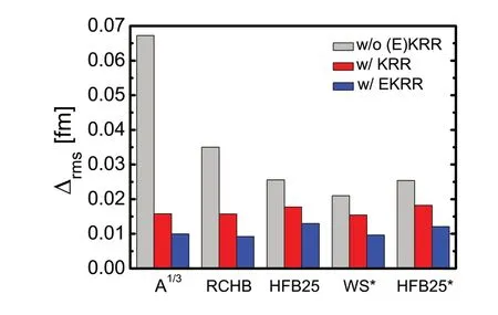
Fig.1 (Color online) The RMS deviations between the experimental data and the predictions of five different models with and without the KRR/EKRR method
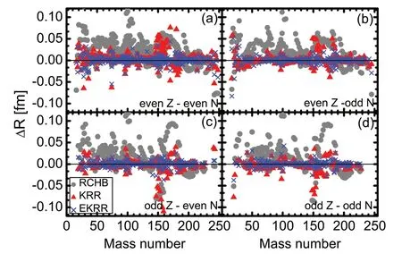
Fig.2 (Color online) Radius differences ΔR between the experimental data and the calculations of the RCHB model (grey solid circles), the KRR method (red triangles), and the EKRR method (blue crosses) for a even—even, b even—odd, c odd—even, and d odd—odd nuclei
To investigate the extrapolation abilities of the KRR and EKRR methods for neutron-rich regions, the 1014 nuclei with known charge radii were redivided into one training set and six test sets as follows: For each isotopic chain with more than nine nuclei, the six most neutron-rich nuclei were selected and classified into six test sets based on the distance from the previous nucleus.Test set 1 (6) had the shortest(longest) extrapolation distance.This type of classification is the same as that used in our previous study [70].The hyperparameters obtained by leave-one-out cross-validation in the KRR/RKRR method remained the same in the following calculations.
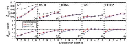
Fig.3 (Color online) Comparison of the extrapolation ability of the KRR and EKRR methods for the neutron-rich region by considering six test sets with different extrapolation distances.The upper panels a—e show the RMS deviations of the KRR and EKRR methods.The lower panels f—j show the RMS deviations scaled to the corresponding RMS deviations for these five models without KRR/EKRR corrections
RMS deviations of the KRR and EKRR methods for different extrapolation steps for the five models are shown in Fig.3a—e.A clearer comparison of the RMS deviations scaled to the corresponding RMS deviations of the five models without KRR/EKRR corrections is shown in Fig.3f—j.Regardless of whether the KRR or EKRR method is considered, the RMS deviation increased with the extrapolation distance.For theA1∕3formula and the RCHB model, the KRR/EKRR method could improve the radius description for all extrapolation distances.For the other three models,the KRR method only improved the radius description for an extrapolation distance of one or two, which could be further improved after considering the odd—even effects with the EKRR method.This indicates that the KRR/EKRR method loses its extrapolation power at extrapolation distances larger than 3 for these three models.It is because the calculated charge radii in these models were quite good and their RMS deviations were already sufficiently small.The KRR/EKRR method automatically identifies the extrapolation distance limit owing to the hyperparametersσandσoebeing optimized using the training data.References [73, 74]demonstrated that the KRR and EKRR methods lose their predictive power at larger extrapolation distances (approximately six), when predicting the nuclear mass using the mass model WS4 [81].This may be due to much more mass data existed than the charge radii, and the KRR/EKRR networks can be trained better with more data.In general, the EKRR method has a better predictive power than the KRR method for an extrapolation distance of less than 3.For an extrapolation distance greater than 3, the results of the KRR and EKRR methods were similar in most cases.Almost none of these extrapolations exhibited overfitting, except for WS*at an extrapolation distance of 3, and this overfitting was quite small.This indicates that both the KRR and EKRR methods have good extrapolation powers and can avoid the risk of overfitting to a large extent.
The observation of the strong OES of the charge radii throughout the nuclear landscape provides a particularly stringent test for nuclear theory.To examine the predictive power of the EKRR method, which is improved by considering the odd—even effects compared with the original KRR method, in the following we will investigate the recently observed OES of the radii in calcium and copper isotopes[14—16].Similar to the gap parameter, the OES parameter for the charge radii is defined as:
wherer(Z,N) is the RMS charge radius of a nucleus with proton numberZand neutron numberN.
Figure 4 compares the experimental and calculated OES for radiiof the calcium (left panels) and copper (right panels) isotopes.The experimental data show that for the calcium isotopes (Fig.4a—e) strong OES exists betweenN=20 and 28 and that a reduction in the OES appears forN≥28.Only RCHB theory could reproduce the trend of the experimental OES without KRR/EKRR corrections.However, the amplitude of the calculated OES was significantly less pronounced than that of the experimental data.Interestingly, after considering the KRR corrections, the calculated OES worsened forN <28 , particularly the phase of the OES became opposite to that of the data.TheA1∕3-formula had no OES over the entire isotopic chain and the WS*model has a weak OES except at theN=20 and 28 shell closures.The OES in the HFB25 and HFB25*models were slightly higher.However, they were still weak compared with the data.Note that although OES can be obtained in the WS*, HFB25 and HFB25*models, the phases of the calculated OES are opposite to those of the experimental data.Considering the KRR method, the OES in these four models increased, particularly for the WS*and HFB25*models for which the calculated OES were stronger than those of the data.However, the OES in these models were still opposite to those in the data.Therefore, although the KRR method improves the description of the charge radius to a large extent, it was difficult to reproduce the observed OES.After considering the EKRR method, the experimental OES values could be reproduced quite well, especially for theA1∕3formula and RCHB theory.For copper isotopes (Fig.4f—j), this situation is similar to that of the calcium isotopes.However, the description of Cu isotopes is not as accurate as that of Ca isotopes when considering the EKRR corrections.The OES is overestimated in all these calculations forN <33 andN>46.In addition, the phases of the OES betweenN=38—40 were not well reproduced.However, the EKRR approach can improve the description of OES to a large extent compared with the original theory.This indicates that after considering the odd—even effects, shell structures and many-body correlations, which are important for OES, can be learned well using an EKRR network.

Fig.4 (Color online) Comparison of experimental and calculated OES of the charge radii ( Δ(3)r ) of the calcium (left panels) and copper (right panels) isotopes.The experimental data are shown as black squares.The calculation results of these five models are shown as grey solid circles, and the calculation results of the KRR and EKRR models are shown as red triangles and blue crosses, respectively
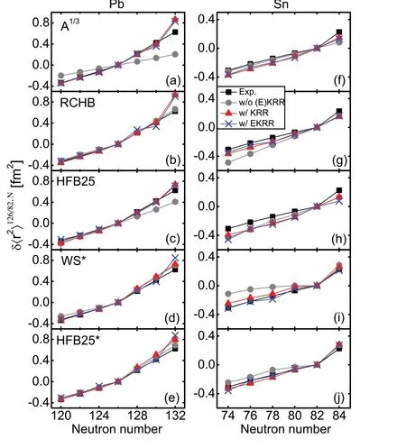
Fig.5 (Color online) Comparison of experimental and calculated differential mean-square charge radius δ〈r2〉N′,N =〈r2〉N -〈r2〉N′for some even—even a—e Pb (relative to 208Pb, =126 ) and f—j Sn(relative to 132Sn, =82 ) isotopes.The experimental data are shown as black squares.The results of these five models are shown as grey solid circles, and the calculation results of the KRR and EKRR models are shown as red triangles and blue crosses, respectively
Similar to OES, abrupt kinks across the neutron shell closures provide a particularly stringent test for nuclear theory.In the present study, Pb and Sn isotopes were considered as examples for investigating the kinks across neutronN=126 and 82 shell closures.Figure 5 compares the experimental and calculated differential mean-square charge radiiδ〈r2〉N′,N=〈r2〉N-〈r2〉N′for some eveneven Pb (Fig.5a—e) (relative to208Pb,N�=126 ) and Sn(Fig.5f—j) (relative to132Sn,=82) isotopes.It can be observed that for Pb isotopes the RCHB theory can reproduce the kink atN=126 perfectly (Fig.5b).In theA1∕3formula and HFB25 model, there is no kink (Fig.5a, c).The kink could be reproduced using the WS*and HFB25*models, but with a slight overestimation (Fig.5d, e).The results obtained by considering the KRR and EKRR methods were similar.There are several interpretations of kinks[50, 82—85].Our results indicate that kinks may not be connected to odd—even effects, such as pairing correlations.The well-reproduced kinks also provide a test of the proposed KRR/EKRR method.The kinks atN=126 in all five models could be reproduced quite well, but the calculated differential mean-square charge radius atN=132 was too large compared with the data.For the Sn isotopes,only the WS*and HFB25*models reproduced the kink atN=82.However, the absolute values of the calculatedδ〈r2〉 fromN=74-78 are small compared with the data,especially for the WS*model.After applying the KRR/EKRR method, the results reproduced the data quite well.It also can be seen that the KRR/EKRR corrections to theA1∕3formula and HFB25 model are inconspicuous.Therefore, the kink atN=82 cannot be reproduced using the KRR/EKRR method.For the RCHB model, the differential mean-square charge radii calculated fromN=74 to 80 were improved, and a kink appeared, but was still slightly weaker compared with the data.
5 Summary
In summary, the extended kernel ridge regression method with odd—even effects was adopted to improve the description of the nuclear charge radius by using five commonly used nuclear models.The hyperparameters of the KRR and EKRR methods for each model were determined using leave-one-out cross-validation.For each model, the resultant root-mean-square deviations of the 1014 nuclei with proton numberZ≥8 could be significantly reduced to 0.009-0.013 fm after considering a modification with the EKRR method.The best among them was the RCHB model, with a root-mean-square deviation of 0.0092 fm,which is the best result for nuclear charge radii predictions using the machine learning approach as far as we know.The extrapolation abilities of the KRR and EKRR methods for the neutron-rich region were examined and it was found that after considering odd—even effects, the extrapolation power could be improved compared with that of the original KRR method.Strong odd—even staggering of nuclear charge radii in Ca and Cu isotopes was investigated and reproduced quite well using the EKRR method.This indicates that after considering the odd—even effects, shell structures and many-body correlations can be learned quite well using the EKRR network.Abrupt kinks across the neutronN=126 and 82 shell closures were also investigated.
Author ContributionsAll authors contributed to the study conception and design.Material preparation, data collection and analysis were performed by Lu Tang and Zhen-Hua Zhang.The first draft of the manuscript was written by Lu Tang and all authors commented on previous versions of the manuscript.All authors read and approved the final manuscript.
Data availability statementThe data that support the findings of this study are openly available in Science Data Bank at https:// cstr.cn/ 10.57760/ scien cedb.j00186.00357 and https:// www.doi.org/ 31253.11.scien cedb.j00186.00357.
Declarations
Conflict of interestThe authors declare that they have no competing interests.
 Nuclear Science and Techniques2024年2期
- Nuclear Science and Techniques的其它文章
- Measurement of the neutron-induced total cross sections of natPb from 0.3 eV to 20 MeV on the Back-n at CSNS
- Unbound 28 O, the heaviest oxygen isotope observed: a cutting-edge probe for testing nuclear models
- Development of CONTHAC-3D and hydrogen distribution analysis of HPR1000
- Total ionizing dose effect modeling method for CMOS digital-integrated circuit
- A fast forward computational method for nuclear measurement using volumetric detection constraints
- Artificial neural network-based method for discriminating Compton scattering events in high-purity germanium γ-ray spectrometer