Artificial neural network-based method for discriminating Compton scattering events in high-purity germanium γ-ray spectrometer

Chun-Di Fan · Guo-Qiang Zeng · Hao-Wen Deng · Lei Yan · Jian Yang · Chuan-Hao Hu · Song Qing ·Yang Hou

Abstract To detect radioactive substances with low activity levels, an anticoincidence detector and a high-purity germanium (HPGe)detector are typically used simultaneously to suppress Compton scattering background, thereby resulting in an extremely low detection limit and improving the measurement accuracy.However, the complex and expensive hardware required does not facilitate the application or promotion of this method.Thus, a method is proposed in this study to discriminate the digital waveform of pulse signals output using an HPGe detector, whereby Compton scattering background is suppressed and a low minimum detectable activity (MDA) is achieved without using an expensive and complex anticoincidence detector and device.The electric-field-strength and energy-deposition distributions of the detector are simulated to determine the relationship between pulse shape and energy-deposition location, as well as the characteristics of energy-deposition distributions for fulland partial-energy deposition events.This relationship is used to develop a pulse-shape-discrimination algorithm based on an artificial neural network for pulse-feature identification.To accurately determine the relationship between the deposited energy of gamma (γ) rays in the detector and the deposition location, we extract four shape parameters from the pulse signals output by the detector.Machine learning is used to input the four shape parameters into the detector.Subsequently, the pulse signals are identified and classified to discriminate between partial- and full-energy deposition events.Some partial-energy deposition events are removed to suppress Compton scattering.The proposed method effectively decreases the MDA of an HPGe γ-energy dispersive spectrometer.Test results show that the Compton suppression factors for energy spectra obtained from measurements on 152Eu, 137Cs, and 60Co radioactive sources are 1.13 (344 keV), 1.11 (662 keV), and 1.08 (1332 keV),respectively, and that the corresponding MDAs are 1.4%, 5.3%, and 21.6% lower, respectively.

Keywords High-purity germanium γ-ray spectrometer · Pulse-shape discrimination · Compton scattering · Artificial neural network · Minimum detectable activity

1 Introduction

The incomplete deposition of gamma (γ)-ray energy in a detector increases the Compton background count in γ-ray spectra [1, 2] and reduces the peak-to-Compton ratio, which adversely affects qualitative and quantitative spectral analyses.The anticoincidence technique is typically used for Compton suppression [3—8].However, one or more anticoincidence detectors with electronic circuits are required,which increases the system volume, equipment complexity,and maintenance costs.Pulse-shape discrimination (PSD)has been used for Compton suppression [9—14] and can decrease Compton scattering background without requiring an anticoincidence detector or electronic circuits.The instrument used for PSD can be designed and manufactured via a simple process, is low maintenance, and features a low failure rate and low cost.PSD is widely applicable to portable and laboratory radiation-detection instruments.Therefore, an increasing number of researchers are using PSD to suppress background Compton scattering.

Classical PSD methods, such as those based on the ratio A/E of the maximal current signal amplitude A to the event energy E, the trailing edge of a current waveform, and the rising-time ratio of a charge waveform [13—15], can achieve background suppression by screening single- and multi-point events to enhance the peak-to-Compton ratio of the energy spectrum [16—19].However, background suppression is typically accompanied by decreased full-energy peak counts.To reduce the minimum detectable activity (MDA), deducting the background without or with less loss of full-energy peak counts is difficult as it requires the accurate screening of event types.Simulation and experimental studies show that the pulse shape output by a preamplifier is not only affected by single- and multi-point events [20—22] but also depends significantly on the energy-deposition location in the detector [23—28].Thus, the difference in the energy-deposition location affects the accuracy of eventtype identification.In the low-energy zone of a detector,the photoelectric effect will likely occur; in this regard,the removal of single-point events increases the likelihood of removing full-energy deposition events when the conventional PSD is used [29].In fact, applying the PSD method to high-purity germanium (HPGe) detection systems has not yielded good results in terms of background suppression in low-energy regions.In addition, the pulse waveform reflects various physical factors, such as the interaction type and energy deposition location, and presents a certain degree of complexity [30—33].Multiple physical features of a waveform can describe the waveform shape more finely and provide more effective information for event-type identification, thus improving the accuracy of event-type identification.

In this study, the relationship between pulse shape and energy-deposition location is determined, and the energy deposition location is used to discriminate the event type.The multiparameter concept is introduced to provide more effective information for event-type identification, and an artificial neural network is used simultaneously to screen the event types, thus effectively improving the accuracy of event-type identification, enhancing the peak-to-Compton ratio of the energy spectrum, and reducing the MDA via a significant subtraction in Compton scattering background counts while preserving most full-energy peak counts.

2 Method and simulation

2.1 Detector modeling

SolidStateDetectors.jl [34] was used to model and simulate the HPGe detector to investigate the relationship between pulse shape and energy-deposition location.The coaxial type HPGe detector featured a diameter of 63.6 mm, a height of 59.8 mm, an electrode diameter of 7.5 mm, and an electrode height of 43.5 mm.The three-dimensional structure is shown in Fig.1.The anode potential, cathode potential, and bias voltage were 0, - 2200, and 2200 V, respectively.The operating environment temperature was set to 78 K.A cylindrical impurity concentration distribution model that varied radially and vertically with a central impurity concentration of 5.8 × 109atoms·cm-3and an impurity concentration near the cylindrical edge of ～ 6.2 × 109atoms·cm-3was configured as a parameter in the simulation environment.

2.2 Field-strength simulation

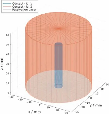
Fig.1 Three-dimensional structure of high-purity germanium detector

whereρ(→r) represents the spatial charge density,ε0represents the dielectric constant, andεrrepresents the relative dielectric distribution.

The open-source software package SolidStateDetectors.jl solves for the electric potential and electric-field strength in each grid within the detector using the equation above via the successive over-relaxation (SOR) algorithm.It obtains the values of the electric potential and electric-field strength and visualizes their distributions, and then generates contour plots for the equipotential and electric-field lines.The results are shown in Fig.2.

To calculate the weighting potential distribution of the germanium crystal and determine the induced signals on the electrodes during charge-carrier drift, we solved the weighted potentialϕ(→r) using the Poisson equation with boundary conditions by assuming that the weight potentials of the anode and cathode are 1 and 0 V, respectively.

Ccolrepresents the collecting electrode andCuncolrepresents the non-collecting electrode.By setting the space charge to zero, the weighting-potential distribution inside the detector was obtained via multiple iterations of the SOR-solving calculations, as shown in Fig.3.

Fig.2 Distributions of a potential, b potential with equipotential lines, c electric-field strength, and d electric-field strength with electric-field lines of high-purity germanium detector

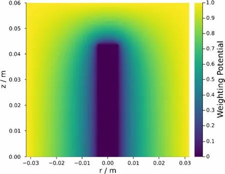
Fig.3 Weighting-potential distribution of high-purity germanium detector

2.3 Drift-velocity model

The relationship between the drift velocity vectorand electric field vectorexpressed as follows:

Owing to the band structure of Ge crystals, the conductivity is anisotropic at high electric fields and low temperatures.This anisotropy results in different drift velocities of charge carriers in different directions relative to the crystal axes.Moreover, if the electric-field direction is not aligned with the crystal’s rotational symmetry axis, then the drift velocity will have a nonzero angle relative to the applied electric field.The drift velocitiesalong the ＜ 100 > , ＜ 110 > ,and ＜ 111 > crystal axes can be described as follows [35—37]:

where the scalaru0represents the mobility in low electric fields;represents the electric field strength; andE0,βandunare used to adjust the drift velocity.

Under a low electric-field strength (0.1 kV/cm ≤E≤ 3 kV/cm), the Gunn effect is negligible and the mobility becomes isotropic.The fitting parameteru0for mobility is independent of the crystal’s orientation, and the formula for velocity can be simplified as shown in Eq.(4).However,whenE≥ 3 kV/cm, the Gunn effect becomes significant,which necessitates the incorporation of the termunEto theformula for correction.The Advanced GAmma Tracking Array (AGATA) collaboration determined the values of the parameters in the empirical formula for drift velocity under experimental conditions, as listed in Table 1 [36, 37].These parameters can be configured in the configuration file of ADLChargeDriftModel, and SolidStateDetectors.jl utilizes these parameters to accurately simulate the migration velocity of charge carriers, thereby facilitating precise simulations.

Table 1 Drift-velocity model parameters developed by AGATA collaboration

2.4 Waveform simulations

In the waveform simulation, the drift velocity of charge carriers at various positions within the detector was calculated based on the distribution of the electric-field strength and drift-velocity models.The initial positions and time steps of the charge carriers were specified, and the drift trajectories of the charge carriers were computed.Finally, by combining the drift trajectories with the weighting potential in accordance with the Shockley—Ramo theorem, the charges induced on the electrode were calculated and then converted into voltage pulse waveforms.During the waveform simulation,the charge carriers were regarded as ideal point charges.

Based on the weighting potential distribution and drift velocities of charge carriers at various positions within the Ge crystal, the Shockley—Ramo theorem can be used to calculate the signal waveform induced on the readout electrode in the detector, owing to the drift of charge carriers along their trajectories [38].For an electron—hole pair created by energy deposition at pointrwith an equal and opposite static chargeq, the electron- and hole- drift trajectories are denoted asreandrh, respectively.The induced chargeQ(t)at the electrode at time t is calculated as follows:

where ϕ represents the weighting potential at the positions ofreandrhon the electrode at timet.

The simulated waveform amplitudes are expressed in units of charge,e0.In a charge-sensitive preamplifier, the charges induced on the detector electrode are integrated into the feedback capacitor and converted into voltage signals.Meanwhile, a continuous discharge occurs on the feedback resistor.The output voltage of the preamplifierUout(t) can be represented as shown in Eq.(7).

The waveforms at multiple positions along the axial and radial directions of the detector were simulated and analyzed.Along the positive direction of the cylindrical axis,the initial height of the charge carriers was set from 44.5 to 59.5 mm, with a step size of 1 mm for each waveform simulation.This resulted in waveforms at 16 positions, as shown in Fig.4a.At a height of 25 mm along the cylindrical axis, the initial position of the charge carriers was set from 4.5 to 30.5 mm along the radial direction of the cylinder,with a step size of 2 mm for each waveform simulation.This resulted in waveforms at 14 positions, as shown in Fig.4b.

Three representative waveforms were selected from the axial and radial directions to compare their shapes, as shown in Fig.4c and d.In both directions, the energy-deposition location significantly affected the pulse-waveform shape.The pulse waveform generated near the cathode exhibited a fast-to-slow rise time.By contrast, the pulse waveform generated near the anode exhibited a slow-to-fast rise time.The pulse waveform generated at an intermediate depth exhibited a fast-to-slow-to-fast rise time, thus presenting a reverse “S”shape.

2.5 Analysis of charge-cloud effect

The motion of electrons and holes is not solely determined by external electric-field forces.In fact, the diffusion and self-repulsion of charge carriers contribute significantly to carrier drift.To simulate this phenomenon, electrons and holes are no longer described as single point charges but as charge clouds composed of multiple point charges.This model incorporates both diffusion and self-repulsion.Diffusion is used to model the random thermal motion of charge carriers, whereas self-repulsion describes the repulsive interaction between charge carriers of the same type.This model does not consider the attraction between electrons and holes.

In SolidStateDetectors.jl, two options are available for charge distribution.For a charge cloud composed of a few charges (less than 50), the shell comprises a Plato polyhedron, and point charges are distributed on the vertices of the polyhedron.For a charge cloud with more charges (more than 50), the point charges are distributed uniformly on a regular spherical surface.

The number of charge carriers generated by energy deposition in a high-purity Ge detector is calculated as follows:

wherenis the number of charge carriers generated by energy deposition,Ethe deposited energy, andωthe ionization energy.

At the liquid nitrogen temperature (77 K), the average ionization energy of high-purity Ge is approximately 3 eV.In the simulation, the energies deposited in the detector were set to 344, 662, and 1332 keV.Using these number and Eq.(9), the number of generated charge carriers were calculated to be approximately 114,667, 220,667, and 444,000,respectively.Therefore, in the simulation, the charge-distribution model was set as point charges distributed uniformly on a regular spherical surface.Meanwhile, the parameter used to pass the total charge quantity in the NBodyCharge-Cloud function was set to the respective values mentioned above to transmit the total charge quantity.

At positionZ= 58.5 mm on the axis (approximately 1.3 mm from the top anode of the detector), the differences in the induced charge waveforms on the electrode are as shown in Fig.5a for the cases with and without the chargecloud model.When electrons drifted toward the anode under the effect of an electric field, the electrons that were initially in close proximity to the anode reached the latter first.Meanwhile, holes drifted toward the cathode under an electric field, and because they were initially farther from the cathode, they arrived later.

For the point-charge model, the numerous electrons generated was regarded as a point arriving at the electrode at a certain moment, thus resulting in a rapid increase in the signal at the anode.By contrast, in the charge-cloud model,the numerous electrons were distributed in a spherical shape.The electrons near the boundary of the spherical cloud on the side closer to the anode reached the electrode first, followed by the electrons near the center of the sphere, and finally,the electrons near the boundary on the side farther from the anode.Consequently, the number of electrons reaching the electrode increased gradually, thus resulting in a relatively slow change in the amplitude of the induced charge on the anode compared with the case of the point-chargemodel.The subtraction of the charge waveforms between the two models generated the first pulse, as shown in Fig.5b.This process is similar to that of the drift of holes toward the cathode, which resulted in a second pulse, as shown in Fig.5b.Owing to the slower drift velocity of the holes, the rate of change in the amplitude of the induced charge during the acquisition process by the electrode was lower for the charge-cloud model compared with that when electrons were acquired.Therefore, the pulse amplitude, after subtracting the charge waveforms between the two models, was larger for the acquired holes.

Fig.4 Simulated pulse waveforms corresponding to multiple energydeposition locations in a axial and b radial directions, and three typical pulse waveforms generated at different positions in c axial and d radial directions

In summary, the different models resulted in certain differences in the spatial distribution of the charge carriers,thereby causing slight differences in the induced charge waveforms during the drift of charge carriers toward the electrode.

In the simulation, when the charge-distribution model was set as the charge-cloud model, certain changes were observed in the waveform of the induced charge, unlike the case for the point-charge model.We calculated the charge waveforms generated on the electrodes under both models, subtracted them to extract the maximum difference in charge quantity, and then analyzed the results.Simulations were conducted under deposition energies of 344, 662,and 1332 keV at points along the axis fromz= 44.5 mm toz= 58.5 mm at 1 mm intervals.The charge waveforms for both models were calculated, and the maximum difference in the charge quantity was plotted as a scatter plot, as shown in Fig.6a.

As shown, the change in position did not affect the maximum difference in the charge quantity in either model.However, as the deposition energy increased, the maximum difference in the charge quantity increased under both models.This is because, in the charge-cloud model, as the number of carriers increased, the radius and distribution density of the charge cloud increased as well.As the radius increased,a longer time was required for the charge cloud to be completely acquired by the electrode.As the distribution density increased, the cardinality of the charge cloud increased, thus resulting in a greater difference in the charge quantity under both models during the same acquisition process.

Figure 6b shows the maximum relative error as a measure of the effect of the charge-cloud model on the pulse waveform.As shown, the maximum relative error was less than 5% in the range fromz= 45.5 mm toz= 57.5 mm.In the region near the electrodes where energy deposition occurred,the relative error increased.This is because an electron or hole cloud was rapidly acquired by the electrode when the energy-deposition position was close to the electrode.The waveform values were lower when the charge quantity reached its maximum difference.As these lower waveform values were used as the denominator for calculating the maximum relative error, a relatively higher calculated value was obtained.However, the values of these relative errors remained less than 10%.Based on the analysis above,the effect of the charge-cloud model on the waveform shape can be considered negligible.

2.6 Simulation of energy-deposition location

We considered two types of events, i.e., full- and partialenergy deposition.In this section, we determine the relationship between the energy-deposition location and event type.This relationship is used to discriminate between the two event types based on the difference in the distribution of the energy-deposition location.We used the GEometry ANd Tracking (GEANT4) simulation software package [39—41]developed by the European Organization for Nuclear Research to simulate the interaction process of 344-, 662-and 1332-keV rays from152Eu,137Cs, and60Co radioactive sources entering a coaxial HPGe detector, respectively [42].In the GEANT4 environment, QBBC is registered as a physics list, including the GEANT4 electromagnetic (G4EM)standard physics package and GEANT4 decay physics(G4DecayPhysics) physics package.A detector model was established using an N-type coaxial HPGe detector used in the laboratory as a prototype.The diameter and height of the Ge crystal were 63.3 and 59.8 mm, respectively.A 0.6-mm-thick aluminum sheet placed 6.3 mm from the top of the Ge crystal was used to simulate the aluminum shell of the detector.A 300-nm-thick borided layer was used as a thin window on top of the Ge crystal.The dimensions and positions of the HPGe crystal and aluminum shell are shown in Fig.7a.The radiation source was a circular planar source centered on the detector axis, with a diameter of 63.3 mm.It was located 40 mm above the surface of the detector.During the simulation, 200,000 gamma rays with energies of 344, 662, and 1332 keV were emitted along the negative z-axis as incident rays.The initial positions and directions of the gamma-rays are shown in Fig.7b.In the GEANT4 simulation, the gamma rays first passed through the aluminum casing and thin window and then interacted with the Ge crystal.The transport processes, reaction types,and interaction points at the step level inside the Ge crystal were statistically analyzed in the simulation.For each event,conditional statements were used to select events with partial-energy and full-energy depositions, as well as to extract the coordinates of the final energy deposition.Event-type selection and coordinate extraction were performed using the GEANT4 program file SteppingAction.cc.The selection criteria for the event types are described below.

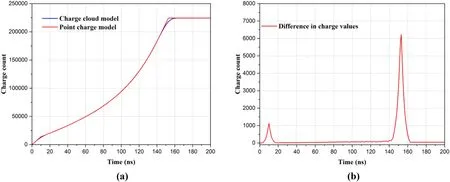
Fig.5 a Charge-pulse waveforms output from electrode using cloud-charge and point-charge models under 662 keV of deposition energy.b New waveform obtained by subtracting the two pulse waveforms

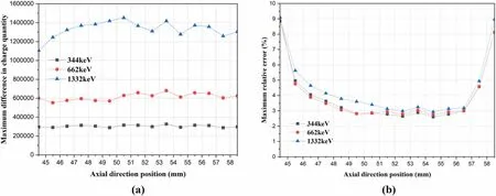
Fig.6 a Trend of maximum charge difference in pulse waveforms generated by two models with energy depositions at different positions, for energy depositions of 344, 662, and 1332 keV.b Trend of maximum relative error with respect to energy-deposition position

Partial-energy deposition event criteria: The previous energy-deposition position was within the Ge crystal, the subsequent ray passed through the boundary between the germanium crystal and medium material, and the kinetic energy of the ray passing through it exceeded 0.

Full-energy deposition event criteria: The previous energy-deposition position was within the Ge crystal, and the kinetic energy of the subsequent ray was 0.

After the simulation, the number of incident rays, total number of energy-deposition events, number of full-energy deposition events, and number of partial-energy deposition events were recorded.The results are summarized in Table 2.The coordinate values of the two types of events were processed into radii and heights, thus resulting in the position distribution of the interactions in the HPGe detector for both types of events, as shown in Fig.8.

The simulation results showed that the full-energy deposition events occurred primarily deep in the detector,whereas the partial-energy deposition events occurred primarily at the detector surface.Thus, we can identify the event type based on the deposition location of γ-ray energy in the detector.

In this section, we analyze the relationship among the pulse shape, energy deposition location, and event type, as well as the mechanism that causes the interconnection of these three factors.

Fig.7 a Model of coaxial HPGe detector simulated using GEANT4.b Energy-deposition process of gamma rays in HPGe detector

3 Data-processing algorithm

More accurate event identifications can be achieved by combining the PSD method with machine learning.A PSD algorithm based on the pulse-feature recognition of artificial neural networks (ANNs) was proposed.This algorithm utilizes four features of the pulse signal’s leading-edge waveform as decision parameters.The four features of the pulse waveform provide useful information for event-type identification, thus resulting in more accurate event-type identifications.These four features contribute differently to event-type identification,i.e., the features have different weights.Manually allocating weights to the decision parameters reasonably is challenging.Therefore, machine learning was employed to train the ANN.The training algorithm enables continuous improvement to the weights in the network.The model with optimal weights exhibits the highest accuracy for discriminating the event type and thus the best performance for discriminating Compton scattering events.The model training process comprises three stages.In the first stage, the effective range of the leading edge is determined from the pulse signals.In the second stage, the PSD algorithm is used to extract the four decision parameters from the effective range of the leading edge.In the third stage,an ANN model and a dataset are constructed.

3.1 Data stripping

Gamma rays deposit energy in the detector, thus generating electron—hole pairs that undergo drift under the effect of an electric field, which is manifested in the rising phase of the charge-sensitive preamplifier output.Therefore, we extracted the leading-edge waveform from the original waveform for analysis.The total number of sampling points for each leadingedge waveform is denoted asNTotal.Before applying the PSD algorithm, we preprocessed the leading-edge waveform.

The amplitude of the leading edge of the pulse signal,PAMP, is calculated as the peak amplitudePPEAKminus the baseline amplitudePBASE.

A prescribed percentage of the leading-edge amplitude was extracted to obtain an effective signal range to reduce noise interference and prevent the time walking of the amplitude[43].The dynamic upper limitTHUPand dynamic lower limitTHLWwere used to obtain the effective signal range as follows:

whererUPandrLWare the upper and lower percentages of the leading-edge amplitude, respectively.In this study,rUPandrLWwere set to 90% and 10%, respectively, to calculate the dynamic threshold, and the resulting effective signalrange is shown in Fig.9.The gain of the digital signal was approximately 12.6 LSB/keV, where LSB denotes the least significant bit of the ADC.

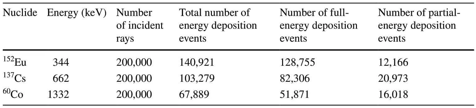
Table 2 Data statistics obtained from GEANT4 simulation

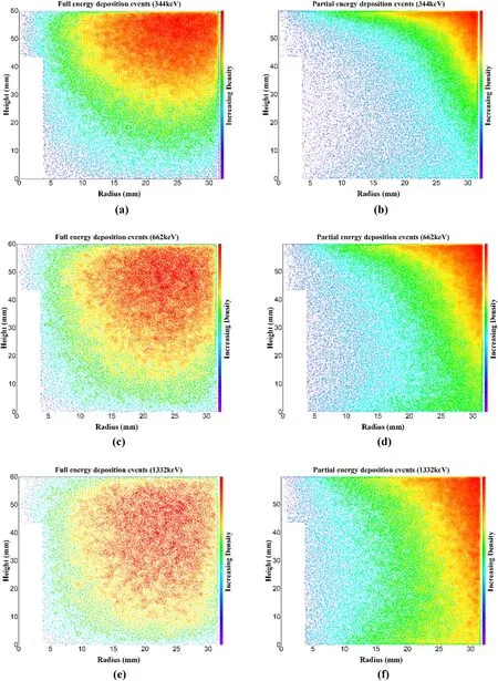
Fig.8 Distribution of locations of full-energy deposition events ((a), (c) and (e)) and partial-energy deposition events ((b), (d) and (f)) corresponding to interaction of 344-, 662- and 1332-keV γ-rays with detector

However, for small-amplitude signals, the baseline noise may trigger a lower threshold before the leading edge of the signal, as shown in Fig.9b.To prevent such false triggers,we used a reverse signal-sampling sequence to capture the trigger sequence number for the lower threshold and a normal pulse-sampling sequence to capture the trigger sequence number for the upper threshold.The trigger sequence numbers of the upper and lower thresholds must satisfy the following inequality:

whereP[n] denotes the waveform of the leading edge,M′the sequence number in the reverse sampling sequence when the sampling point is slightly less than the lower threshold, andNthe sequence number in the forward-sampling sequence when the sampling point is slightly less than the upper threshold.M′was converted to the corresponding sequence numberMin the forward-sampling sequence using Eq.(15).

After obtaining the sequence numbersMandN, the waveformw[n] within the effective signal range of the leading edge was determined as follows:

3.2 Feature extraction

Processing was performed using the PSD algorithm as follows: First, the slope of the effective signal (which has been extracted, as described in the previous section) was calculated.Subsequently, the corresponding slope amplitude was subtracted from each discrete signal amplitude within the effective signal interval to determine a new set of discrete signals.The decision parameters were set to be the maximum value of the new discrete signal and the corresponding relative position on the curve, as well as the minimum value of the new discrete signal and the corresponding relative position on the curve.The four decision parameters accurately reflected the shape features of the pulse signals.

Many methods, such as curve fitting, can be used to calculate the slope of the leading edge.To simplify signal processing, the slope of the leading edge was calculated as follows:

whereTTOTAL_TIMEis the total time of the effective signal range; andTdenotes the sampling period, i.e., 8 ns.

The discrete signal of the new curvef[n] was obtained by subtracting the discrete value of the slope from the discrete value of the effective range of the leading edge.

The maximum valueCMAXand minimum valueCMINof the curve that reflect the protruding degree (upward and downward) of the effective range of the leading edge were calculated as follows:

Fig.9 a and b show the sampling waveforms at the leading edge and the corresponding upper and lower thresholds, respectively.The equivalent energies of the pulse signals were a ～ 662 keV and b ～ 74 keV, respectively

wherePandQdenote the maximum and minimum points of the curve, respectively.The relative positions ofPandQat the leading edge are expressed as follows:

The maximum upper and lower convex values (CMAXandCMIN, respectively) within the effective range of the leading edge and the corresponding relative positions (RMAXandRMIN, respectively) at the leading edge were used as the four decision parameters for the pulse signals (Fig.10).

3.3 Analysis of the effect of noise on decision parameters

We performed a data analysis on the simulated waveforms to assess the effects of different signal-to-noise ratio (SNR) levels, i.e., 30, 40, and 50 dB, on the decision parameters.We obtained waveforms at 16 positions at 1 mm intervals along the axial direction from 44.5 to 59.5 mm.Different levels of noise were added to the original waveforms to achieve SNRs of 30, 40, and 50 dB for each signal.Subsequently, the PSD algorithm was used to extract the decision parameter values for each signal.The mean square deviation of each decision parameter for each signal group was calculated and plotted as a scatter plot, as shown in Fig.11.The decreasing trend of the mean square deviation with increasing SNR indicates that noise affects the values of the decision parameters.Therefore, system noise must be minimized during the experiment.

3.4 ANN

ANNs are sophisticated and effective classification tools[44] that can be used as classifiers to distinguish pulse shapes.In the experiment, a two-layer feedforward neural network was employed as an ANN model.The model comprised an input layer with four inputs, a hidden layer with 10 neurons, and an output layer with two neurons.The activation function for the hidden layer was a sigmoid function.The Levenberg—Marquardt backpropagation algorithm was used as the training algorithm.The data output from the output layer can be interpreted as the probability of the model predicting the event type as a full-energy deposition event.The structure of the ANN is shown in Fig.12.Based on the four decision parameters extracted from the pulse waveform, the ANN computed the predicted probability of the pulse waveform belonging to a particular event type.A result closer to 1 implies a higher probability that an event belongs to a full-energy deposition event.However, a result closer to 0 implies a higher probability that an event belongs to a partial-energy deposition event.By setting a threshold,events with a prediction above the threshold were retained,whereas events with a prediction below the threshold were excluded to maximize the retention of full-energy deposition events and exclude partial-energy deposition events.

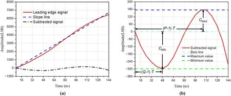
Fig.10 a and b Processing procedure of pulse-shape-discrimination algorithm

Fig.11 Mean square error of effects of different levels of noise on decision parameters

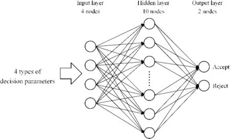
Fig.12 Block diagram of ANN structure

4 Results and discussion

4.1 Detector system

The full-waveform acquisition and analysis system for the HPGe signal used in this study comprised a compartment with a lead shield, a coaxial HPGe detector,a high-voltage module, a signal-conditioning circuit, a full-waveform digital acquisition board, a computer, and upper computer software.A GCDX-40190 N-type coaxial HPGe detector (BSI, Sweden) was used.The detector featured a relative efficiency of 40% and an energy resolution of 1.9 keV@1332 keV.The diameter and height of the HPGe crystal were 63.3 and 59.8 mm, respectively, and the diameter of the cathode was 7.5 mm.The detector was placed in a 10-cm-thick lead compartment, which reduced interference from the environmental background.The lead

compartment contained a copper baffle to obstruct X-rays emitted by lead decay.The radioactive sources used were152Eu,137Cs, and60Co.Three radioactive sources were placed on the surface immediately above the detector for measurement.The cathode and anode biases of the HPGe detector were —2200 and 0 V, respectively.The signalconditioning circuit scaled and adjusted the bias of the pulse signals output from the preamplifier.The full-waveform digital acquisition board with a 16-bit resolution and 125-Msps sampling rate transmitted the acquired waveform data to the computer through the PCIe interface and recorded the data on the storage media.Waveform data from the leading edge of the pulse signal were extracted as original data for subsequent studies.The figures and framework diagram of the system are shown in Fig.13.

4.2 Data preprocessing

A total of 200,000 pulse signals from mixed sources comprising152Eu,137Cs, and60Co were analyzed.Four eigenvalues, i.e.,CMAX,CMIN,RMAXandRMIN, were extracted as decision parameters.Figure 14 shows a dot density map of the distribution of the decision parameters for each track address.The distributions of the decision parameters for the two event types were different and can be used to distinguish the event types.

4.3 ANN training

Different weights were assigned to the four decision parameters to determine the event type.The ANN was extensively trained iteratively on a training dataset to determine the optimum weight factors.A dataset containing correctly classified waveforms obtained from laboratory measurements was prepared to train the ANN via supervised learning.This dataset comprised 207,724 sets of decision parameters extracted from pulse signals generated by the interaction of the detector with γ-rays of152Eu (344 keV),137Cs(662 keV), and60Co (1332 keV) as well as flag values.A total of 29,154 sets of full-energy deposition events within the range of the full-energy peak were assigned a value of 1,and 178,570 sets of partial-energy deposition events within the range of the Compton plateau were assigned a value of 0.The dataset composition is listed in Table 3.The dataset was randomly segmented into three subsets containing 90%,5%, and 5% of the data for training, validation, and testing,respectively.The network was constructed using the neuralnetwork toolbox in MATLAB.The Levenberg—Marquardt backpropagation algorithm was used as the training algorithm, and the initial learning rate was encapsulated in the ANN toolbox.During model training, the learning rate was adaptively adjusted based on the training performance.The network model was trained for 126 epochs on an eight-core workstation.The trained network was employed to classify the events into 89,023 newly sampled and extracted datasets.

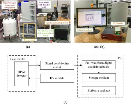
Fig.13 Full-waveform acquisition and analysis system for high-purity Ge signal.a and b Figures and c framework diagram

4.4 Validation of pulse-shape simulation

Simulations were performed to obtain the pulse waveforms generated by the energy deposition of 662 keV gamma rays at multiple positions along the radial and axial directions within the detector.Four decision parameters were extracted from the simulated waveforms and fed into the neural network model for prediction.The depth of the energy-deposition position from the detector surface and the predicted probability values of the event types were plotted as a scatter plot, as shown in Fig.15.In the figure, “probability”represents the probability of an event being predicted as a full-energy deposition event.A higher value indicates a higher probability of a full-energy deposition event, whereas a lower value indicates a higher probability of a partialenergy deposition event.Regardless of the direction (radial or axial), when the depth was small, i.e., at a position close to the detector surface, the predicted probability of a fullenergy deposition event was low.As the depth increased,the predicted probability gradually increased and reached a maximum value at a certain depth, after which the probability value decreased.

The observed trend aligned with the distribution characteristics of full/partial-energy deposition events simulated in GEANT4, as shown in Fig.8.The partial-energy deposition events exhibited a higher probability of being distributed on the outer surface of the detector, whereas the full-energy deposition events showed a higher probability of being distributed in deeper regions of the detector.As the depth increased, the distribution probability reached its maximum value at a certain depth.As the depth with respect to the cathode decreased (i.e., as one approached the cathode),the probability of gamma rays scattering and escaping from the Ge crystal into the cathode increased.Consequently,the probability of full-energy deposition events decreased,which is consistent with the trend presented by the curves shown in Fig.15.

The probability values on the vertical axis in the figure were generally lower than those obtained by inference using the measured waveform value in the experimental environment.This may be attributed to the experimentalenvironment being more complex than the simulation environment, with more factors affecting the pulse waveform,such as the dead layer, hole trapping, and electronic noise.These factors contributed to certain differences between the waveforms observed in the experimental measurements and simulated waveform.However, by training the neural network model based on the decision parameters extracted from the measured waveforms obtained in the experimental environment, and by redefining the thresholds, the same model can be analyzed and inferred from the decision parameters extracted from the simulated waveforms.This indicates that the waveform shapes obtained from boththe simulated and experimental environments exhibited a certain degree of similarity, i.e., the change trend of the waveform-shape characteristics remained consistent with the variation in the energy-deposition positions.

Fig.14 Distribution of decision parameters of pulse signals from mixed radioactive sources comprising 152Eu, 137Cs, and 60Co in corresponding track address

Fig.14 (continued)

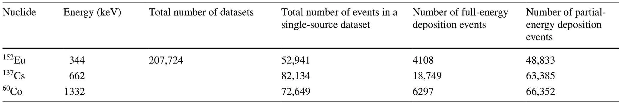
Table 3 Composition of events in training set of neural network model

Fig.15 Scatter plots of probability values against energy-deposition depth for a axial and b radial directions

4.5 Energy-spectrum test

After removing the pulse-signal amplitudes of the Compton scattering events identified by the ANN, those of the remaining events were processed to yield an energy spectrum in which Compton scattering background was suppressed.The suppression of the Compton scattering background was quantified in terms of the Compton suppression factor (FCS) and efficiency (Eff) as follows:

whereP∕CoriginalandP∕CCSare the peak-to-Compton ratios of the energy spectrum before and after Compton suppression using the ANN, respectively; andRP-Pis the ratio of the areas of the full-energy peak in the energy spectrum before and after Compton suppression using the ANN.

The following ratios were calculated: The ratio of the 344-keV full-energy peak height for signals from the152Eu radioactive source to the average height of the Compton continuum at 298—339 keV, the ratio of the 662-keV full-energy peak height for signals from the137Cs radioactive source to the average height of the Compton continuum at 680—730 keV, and the ratio of the 1332-keV fullenergy peak height for signals from the60Co radioactive source to the average height of the Compton continuum at 1040—1096 keV.Figure 16 shows the effects of the threshold value on the Compton suppression factor, peak area ratio,and efficiency.

As the threshold value increased, the Compton suppression factor for the three radioactive sources increased and the peak area ratio decreased.Suppression of the Compton scattering background decreased the count over the full-energy peak range, which decelerated the reduction in the MDA.At a threshold value of 0.03, the Compton suppression factor can be improved while a high full-energy peak count is retained.Table 4 lists the corresponding Compton suppression factors, peak area ratios, and efficiencies.Figure 17 shows the logarithmic energy spectra before and after the suppression of Compton scattering background.

4.6 MDA

The MDA is calculated as follows [45—47]:

whereBis the background count over the full-energy peak range,mthe sample mass,tthe measuring time,εthe absolute detection efficiency of the respective γ-ray, andIthe emission intensity of the γ-ray.

The MDA ratio (a) is defined as the ratio of MDAs before and after the suppression of Compton scattering background for the same measurement.It is used to eliminate the constant in the MDA formula, thereby simplifying the calculation.MDA levels can be effectively decreased foraless than 1.The MDA ratio is computed as follows:

In the equation above, subscripts 1 and 2 denote the parameter values obtained before and after the suppression of Compton scattering background, respectively; andNdenotes the count for the net peak area.

Table 5 shows the MDA ratios for the full-energy peaks of γ-rays from152Eu,137Cs, and60Co, which were calculated based on a threshold value of 0.03.

As shown in Fig.18, this method resulted in a decrease in the MDA for the three energy levels of gamma rays within a certain threshold range.As the gamma-ray energy increased,the maximum reduction in the MDA increased.Considering the optimization effect of the MDA across the entire energy range, a threshold of 0.03 was set.As shown in Table 5, at this threshold, the MDA for the full-energy peaks of gamma rays at 344, 662, and 1332 keV from the 152Eu, 137Cs,and 60Co radioactive sources decreased by 1.4%, 5.3%, and 21.6%, respectively.

5 Conclusions and future work

The proposed method effectively suppressed Compton scattering background over the entire energy range considered.The Compton suppression factors of radioactive sources152Eu,137Cs, and60Co reached 1.13 (344 keV), 1.11(662 keV), and 1.08 (1332 keV), respectively, and the corresponding MDAs decreased by 1.4%, 5.3%, and 21.6%,respectively.The higher the energy of the incident rays,the greater was the reduction in the MDA.This occurred because the distribution of events for the full-energy deposition of high-energy γ-rays was concentrated deep in the detector, which differed considerably from the distribution of partial-energy deposition events.Therefore, although using an ANN removed partial-energy deposition events,more full-energy deposition events were retained as compared with partial-energy deposition events, which reduced the count loss over the range of the full-energy peak and further decreased the MDA.

In addition to coaxial HPGe detectors, systems equipped with broad-energy Ge and small-anode GE detectors can be investigated experimentally to extend the application range of this method.

Fig.16 Effects of threshold value on Compton suppression factor, peak area ratio, and efficiency for energy deposition from a 152Eu, b 137Cs,and c 60Co

Table 4 Compton suppression factor, peak area ratio, and efficiency for 152Eu, 137Cs, and 60Co at threshold value of 0.03

In future studies, we plan to extract additional decision parameters from the leading edge of pulse signals to characterize the edge shape more accurately.The accuracy of the identification and classification of full- and partialenergy deposition events can be improved by increasing the number of hidden layers in the ANN model and the number of neurons in each layer, as well as by improving the activation function and training algorithm, thereby enhancing Compton suppression and decreasing the MDA.

Fig.17 Logarithmic energy spectrum before and after suppression of Compton scattering background

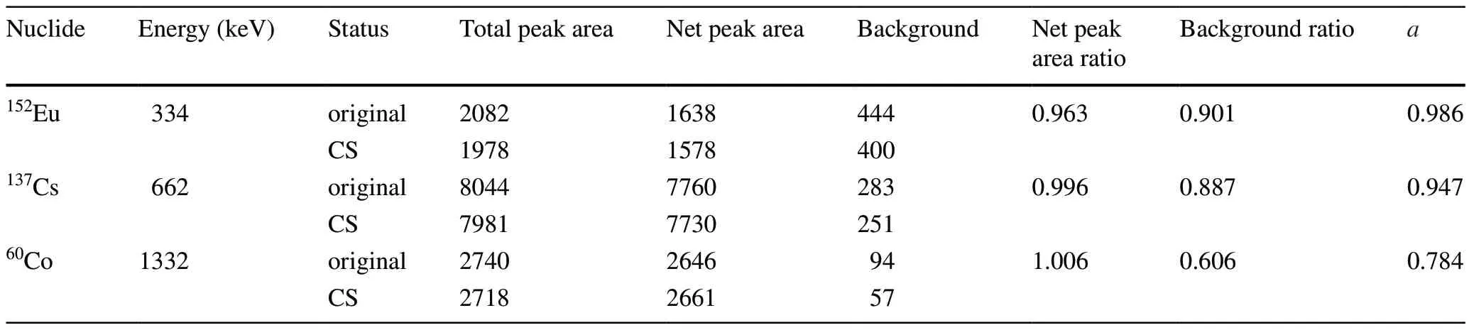
Table 5 MDA ratio for full-energy peak of γ-rays from 152Eu, 137Cs, and 60Co

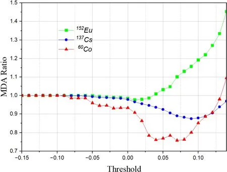
Fig.18 Relationship between MDA ratio and threshold values for three nuclides

Author contributionsAll authors contributed to the study conception and design.Material preparation, data collection and analysis were performed by CDF, GQZ, JY and CHH.The first draft of the manuscript was written by CDF and all authors commented on previous versions of the manuscript.All authors read and approved the final manuscript.Data availabilityThe data that support the findings of this study are openly available in Science Data Bank at https:// cstr.cn/ 31253.11.scien cedb.j00186.00400 and https:// doi.org/10.57760/ scien cedb.j00186.00400.

DeclarationsConflict of interestThe authors declare that they have no competing interests.