Development of mathematically motivated hybrid soft computing models for improved predictions of ultimate bearing capacity of shallow foundations
Abiodun Ismail Lawal, Sangki Kwon
a Department of Energy Resources Engineering, Inha University, Incheon, South Korea
b Department of Mining Engineering, Federal University of Technology, Akure, Nigeria
Keywords:Ultimate bearing capacity (UBC)Geotechnics Grasshopper optimization algorithm (GOA)Salp swarm algorithm (SSA)Soft computing (SC) method
ABSTRACT Ultimate bearing capacity(UBC)is a key subject in geotechnical/foundation engineering as it determines the limit of loads imposed on the foundation.The most reliable means of determining UBC is through experiment, but it is costly and time-consuming which has led to the development of various models based on the simplified assumptions.The outcomes of the models are usually validated with the experimental results, but a large gap usually exists between them.Therefore, a model that can give a close prediction of the experimental results is imperative.This study proposes a grasshopper optimization algorithm (GOA) and salp swarm algorithm (SSA) to optimize artificial neural networks (ANNs)using the existing UBC experimental database.The performances of the proposed models are evaluated using various statistical indices.The obtained results are compared with the existing models.The proposed models outperformed the existing models.The proposed hybrid GOA-ANN and SSA-ANN models are then transformed into mathematical forms that can be incorporated into geotechnical/foundation engineering design codes for accurate UBC measurements.
1.Introduction
Shallow foundation design is significant in the foundation and geotechnical engineering.The safety of the foundation is very paramount as its failure can lead to the loss of lives and property.The two major criteria upon which the design of a shallow foundation is based are ultimate bearing capacity (UBC) and limiting settlements of the foundation(De Beer,1965;Padmini et al.,2008).The UBC relies on the shear strength of soil, and it is usually theoretically determined using the theories of Terzaghi (1943),Meyerhof (1963), Vesic (1973), etc.The theoretical methods of determining UBC are commonly based on the limit equilibrium approach, which is usually statically indeterminate and hence based on simplified assumptions(Lawal,2018,2021;Xu et al.,2019;Xu and Lawal, 2021).
Besides the limit equilibrium approach, the method of characteristics (MoC) known as the slip-line method proposed by Sokolovskii (1965) has also been used to calculate the bearing capacity of the soil(Kumar,2003;Martin,2005;Sun et al.,2013;Han et al.,2016).According to Hjiaj et al.(2005),this method can give a good estimate of the correct solution,but its accuracy is difficult to confirm when one of the bounding properties is unknown.Other methods that have been used to estimate the bearing capacity of soil include conventional numerical method (Frydman and Burd,1997; Loukidis and Salgado, 2009) and limit analysis method(Soubra,1999; Hjiaj et al., 2005; Krabbenhoft et al., 2012).Fenton and Griffiths (2003), Przewłócki (2005), and Chwala (2019)considered the concept of variability in soil properties in their respective conventional numerical, MoC, and limit analyses.He et al.(2021) and Wang et al.(2021) combined the conventional numerical method and soft computing(SC)method to perform the bearing capacity related reliability analyses.The bearing capacity of the footing in multilayer soil has also been studied.For example,Michalowski and Shi (1995) used the kinematic approach of limit analysis to study the bearing capacity of dual-layer granular soil,and Kuo et al.(2009) used numerical formulation of upper and lower bound limit analysis methods to develop multiple regressionand artificial neural network (ANN) models for the analysis of bearing capacity of multilayer soil.The experimental method is the most reliable means of measuring UBC, but it is costly and timeconsuming.Hence, geotechnical engineers still rely largely on theoretical methods for estimating UBC.The results of theoretical methods are usually validated with the existing experimental data.
However, the outcome of the validations revealed a disparity between the theoretical and experimentally measured UBCs.The quest for an accurate model that can mimic the experimentally measured UBC has made the researchers form a database of the existing experimental results and develop artificial intelligence(AI)/SC-based models for predicting UBC(Padmini et al.,2008).This decision may be due to various encouraging performances of the SC models in their various applications in different fields of human endeavour(Wang et al.,2020a;Adesanya et al.,2021;Akinwekomi and Lawal,2021;Lawal et al.,2021a,b,c;Tang and Na,2021;Zhang et al.,2022).Padmini et al.(2008)developed adaptive neuro-fuzzy inference system (ANFIS), ANN, and fuzzy inference system (FIS)models to predict the UBC of cohesionless soil based on the database of the experimental studies by Weiβ (1970), Muhs and Weiβ(1971, 1973), Briaud and Gibbens (1999) and Gandhi (2003).Kalinli et al.(2011) developed ANN and ant colony optimization models based on the database compiled by Padmini et al.(2008).Most recently, Ahmad et al.(2021) used the same experimental database adopted by Padmini et al.(2008)and Kalinli et al.(2011)to develop a Gaussian process regression (GPR)-based model.ANN and ANFIS models have been proven to be more accurate for the UBC prediction based on the studies of Padmini et al.(2008) and Kalinli et al.(2011), but the major issue of concern in the existing models is their practical applicability because of the unavailability of mathematical forms of the models.Hence, the geotechnical engineers still rely on the classical models (e.g.Meyerhof, 1963;Hansen,1970;Vesic,1973).In addition,the computed errors in their validations are still high.Therefore, it is timely and important to propose a mathematical-based SC model for the prediction of UBC with a minimal validation error.
In this study, novel grasshopper optimization algorithm (GOA)and salp swarm algorithm (SSA) optimized ANNs (GOA-ANN and SSA-ANN) are proposed for accurate predictions of UBC.The proposed hybrid ANN models have not been used for the UBC prediction to the authors’ best knowledge.The proposed models are transformed into simple mathematical forms that can easily be used by the geotechnical engineers or included in the geotechnical design codes for the foundation design.The MATLAB code for the implementation of the proposed models is also provided.The performances of the proposed models are evaluated using various statistical indices such as coefficient of correlation(R),coefficient of efficiency (E), root mean squared error (RMSE), mean biased error(MBE), and Akaike information criterion (AIC) and compared with the existing models to establish their suitability for the UBC prediction.
1.1.Brief bibliometric review of the SC methods for prediction of shallow foundation bearing capacity
The data used for this review were mined from the Web of Science Collection which has been identified to be a reliable data source (Aguillo, 2012; Abdeljaoued et al., 2020).Using the keywords‘ultimate bearing capacity’and‘shallow foundations’,about 397 items were identified which contain about 339 articles, 48 proceedings,11 early access,7 review articles,and 5 book chapters.The years of the articles start from 1975 till date.However, the datasets were filtered and limited to the articles that applied AI/machine learning to predict the UBC of shallow foundations on cohesionless soil based on the same database formulated by Padmini et al.(2008).Only about 13 articles met this threshold and were exported and used for the analyses in the VOSviewer.Going by the source of the articles in relation to the country, Iran and China took the lead, each with four articles, while Malaysia, Vietnam,and India have two items each.Poland,Pakistan,Turkey,and the USA have one each.The articles’ co-occurrences based on all keywords were used in the VOSviewer to visualize different key terms or methods that have been used.The obtained result is shown in Fig.1.From Fig.1, ANN,deep neural network, ant colony optimization, ANFIS, FIS, genetic programming, particle swarm optimization, M5, hybrid M5, random forest, chaotic particle swarm optimization, and support vector machine have been used to predict the UBC of shallow foundation based on the existing experimental or laboratory results.The authors that have contributed are Padmini et al.(2008), Zhao and Yin (2010), Kalinli et al.(2011), Samui (2012), Shahnazari and Tutunchian (2012), Tsai et al.(2013), Marto et al.(2016), Kohestani et al.(2017), Khorrami and Derakhshani (2019), Xue and Chen (2019), Khorrami et al.(2020), Ahmad et al.(2021), and Pham et al.(2021).The paper of Padmini et al.(2008)has been cited more than 90 times and is the most cited.From the literature survey, various SC techniques have been used to predict the UBC of shallow foundations using the existing database,however,based on the no-free-lunch theorem of Wolpert and Macready(1997),it is appropriate to try new methods to assess their suitability for the UBC prediction.Hence, novel methods,i.e.GOA and SSA,have been used in this study to optimize the ANN model.The proposed models are transformed into useful mathematical forms to unlock the black-box nature of the ANN.This cannot be found in any of the existing models that adopted ANN for UBC prediction.
1.2.Brief overview of the adopted methods
This section comprises a brief overview of the adopted methods.
(1) ANN
ANN is arguably the most used AI/SC method in engineering and many other fields of human endeavour.The reason could be attributed to its ability to solve many complex problems that the traditional statistical approach cannot solve (Lawal and Kwon,2020).For instance, it can work well in a situation where the relationships between the input and targeted output do not exist or where the parameters follow different distributions.It is a functional approximation and consists of a series of internally connected nodes within its internal domain.Its principle of operations mimics that of the human brain and as a result, it can learn from examples and use the gained experience for future recognition or prediction when similar information to the learned one is transmitted to it (Gurney,1997; Lawal et al.,2021a, b).
Jain et al.(1996)presented different forms of ANN architectures.The feedforward multilayer neural network with backpropagation algorithm is the most used in solving engineering problems,which has at least one hidden layer in conjunction with the input and output layers.According to Lawal and Kwon(2020)and Lawal et al.(2021a), the number of nodes in the input and output layers is a function of the model parameters while that of the hidden layer has no agreed means of determining them in the literature and hence the number of suitable hidden layer nodes for a particular problem is usually determined using trial and error methods.Paneiro et al.(2020) used the AIC (Akaike, 1974) and coefficient of determination(R2)to evaluate the suitable number of hidden neurons in their study, but the number of optimum hidden neurons in their study may not be suitable in another problem.Therefore, different numbers of hidden layer neurons should be tried to obtain theoptimum ANN structure for each problem (Rafiq et al., 2001).However,too many neurons in the hidden layer should be avoided to forestall over-fitting.The training process is very paramount in the ANN model and different algorithms are available for this task.The Levenberg-Marquardt (LM) algorithm is the most used training algorithm.The weights, transfer function, and biases are key terms in ANN simulation/modeling.The mathematical expression showing the relation between the terms is presented in Section 2.2.
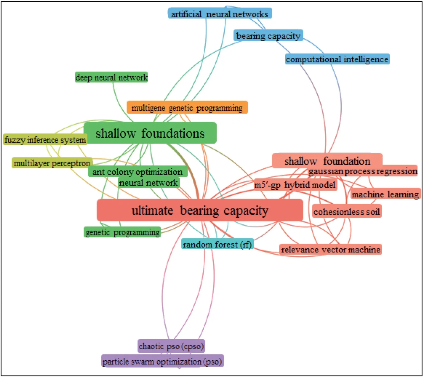
Fig.1.VOSviewer for the keywords.
(2) GOA
Grasshopper is one of the dangerous insects in nature which destroys the vegetation and hurts the agricultural produce.The grasshoppers are said to be one of the largest swarms in creation although they are usually seen individually (Simpson et al.,1999).The life cycle of the grasshopper is in three stages:egg,nymph,and adult.The food source swarming is fascinating characteristic of grasshopper which inspired this optimization algorithm (Rogers et al., 2003; Saremi et al., 2017).Generally, in nature-inspired algorithms,the food source is hunted in stages which are exploration and exploitation stages.In the case of GOA,the exploration process is very fast or rapid while the exploitation is slow.The exploration and exploitation are performed naturally by the grasshopper.They are then modeled by Saremi et al.(2017)to develop the GOA model.The mathematical model explored to simulate the swarming behavior of the grasshopper is presented in the later section.
(3) SSA
SSA, proposed by Mirjalili et al.(2017), is one of the evolutionary-based algorithms that mimic the swarming mechanism of salps in nature.It simulates the mechanism of swarming of salps when gathering wild foods in oceans.In heavy oceans,salps usually form a swarm called salp chain.In SSA,there is only one leader at the head of the chain and the others are followers.Like other evolutionary-based algorithms, the salps are defined in the s-dimensional search space where s stands for the number of variables in each problem.Therefore,the position of all the salps is kept in a 2-dimensional matrix called x.A food source denoted as F is also assumed to exist within the search space which serves as the target of the swarm.The mathematical interpretation of SSA is also presented in the later section.
2.Materials and method
2.1.Data collection
The study was conducted based on the dataset adopted from Padmini et al.(2008).The width of footing(B),depth of footing(D),footing geometry(L/B,where L is the length of footing),unit weight(γ), and internal friction angle (φ) were selected as the input parameters, while the UBC was the only output parameter.The dataset is comprised of 97 data in total which are based on the results of load test results of square,rectangular,and strip footings of different sizes in cohesionless soil of various densities.As previously stated, it was costly and time-consuming to perform experiments.This has made the researchers rely on the existing database for developing AI/SC-based models for predicting the UBC.The statistics of the dataset used are presented in Table 1.The distribution of the dataset was tested, and based on the AIC proposed by Akaike (1974) and Bayes information criterion (BIC) proposed by Schwarz (1978), the width of footing (B) and depth of footing (D) follow lognormal distributions while the remainingparameters (footing geometry L/B, unit weight γ, and internal friction angle φ) are largely uniformly distributed.This is an indication of the high nonlinearity or complexity of model variables,which implies that a model that can handle a highly nonlinear problem will be needed,and such a model is proposed in this study.

Table 1Statistics of the adopted dataset.
2.2.Descriptions of the adopted methods
The ANN, GOA and SSA methods adopted in this study briefly explained in Section 1.2 are further described mathematically below.
(1) ANN
The general mathematical equation for the mechanism of ANN describing the terms stated in Section 1.2 for a typical ANN structure with a single hidden layer is presented as follows (McCulloch and Pitts 1943; Jain et al.,1996):
where y stands for the targeted output(s);x is the input variable(s);w1is the weight connecting the input and output neurons;w2is the weight connecting the hidden and output neurons;b1is the bias in the hidden neurons; b2is the bias in the output neuron(s); and f1and f2are the transfer or activation functions in the hidden and output layers, respectively.The f1is usually a log-sigmoid or hyperbolic tangent while f2can vary between purelin or log-sigmoid or hyperbolic tangent.ANN models are investigated in this study to obtain the most suitable network combinations, and thereafter they are subjected to GOA and SSA.
(2) GOA
The mathematical model explored to simulate the swarming behavior of the grasshopper as obtained by Saremi et al.(2017) is presented below.The position of the grasshopper is defined as
where Xidefines the position of the ith grasshopper,Sidenotes the social interaction, Giis the gravitational force, and Aiis the wind advection.To randomize Eq.(2), the variables on the right-hand side can be multiplied with random numbers between 0 and 1,and thus Eq.(2) becomes
The social interaction Siin Eqs.(2) and (3) can be computed as
where dijrepresents the distance between the ith and jth grasshoppers, which can be computed using dij= |xj- xi|; ^dijis a unit vector from the ith to the jth grasshopper,and^dij=(xj-xi)/dij;and s defines the strength of the social forces and is presented as
where f stands for the attraction intensity, and lais the attractive length scale.
The Giand Aiin Eqs.(2)and(3)can be respectively computed as follows:
where g is the gravitational constant,is a unit vector towards the center of the earth,u is a constant drift,andstands for the unit vector in the wind direction.Replacing Si,Gi,and Aiin Eq.(3)with Eqs.(4), (6) and (7), respectively, Eq.(3) becomes
However, Eq.(8) cannot be used directly for the intending optimization and has therefore been modified as (Saremi et al.,2017):
where ubdand lbdare the upper and lower bounds in the dth dimension, respectively; ^Tdstands for the value of the dth dimension in the target;N is the number of grasshoppers;and c denotes the decreasing coefficient and is given as follows:
where cminand cmaxare the minimum and maximum values,respectively; l is the current iteration; and Litis the maximum number of iterations.More details about the GOA can be found in Saremi et al.(2017).The pseudo-code for implementing the GOA given by Saremi et al.(2017) is presented in Fig.2.
(3) SSA
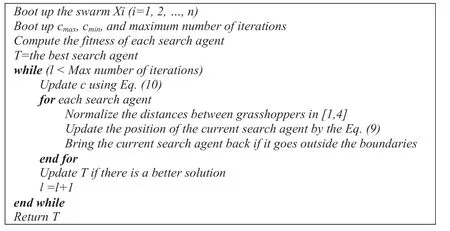
Fig.2.Pseudo-code for the GOA proposed by Saremi et al.(2017).
The mathematical interpretation for SSA obtained from Mirjalili et al.(2017) is given as follows.For the position update, the following equation is utilized:
where xj1depicts the position of the leader in the jth dimension;Fjrepresents the location/position of the food source in the jth dimension;ubjand lbjrepresent the upper and lower bounds in the jth dimension, respectively; and c1, c2, and c3are the random numbers.The implication of Eq.(11) is that the leader changes its position with respect to the food source,and c1is very imperative in SSA as it helps in balancing the exploration and exploitation of the salp.The c1can be computed using the following equation:
The c2and c3are random numbers between 0 and 1, and they dictate the direction of the next position in the jth dimension together with the step size(Mirjalili et al.,2017).The position of the followers can be updated using the following equation based on Newton’s law of motion:
where xijrepresents the position of the follower in the jth dimension; t is the time; v0is the initial speed; and a is the ratio of the final speed to the initial speed,and a = vfinal/v0,in which vfinal=(x - x0)/t.
Since the iteration in optimization is time-dependent and the difference between the iterations is equal to 1, taking v0= 0, Eq.(13) can be modified to
Based on Eqs.(11) and (14), the salp chains can be simulated.The pseudo-code for implementing the SSA is presented in Fig.3(Mirjalili et al., 2017).
2.3.Optimized models proposed
The obtained datasets from the literature were gathered to develop models that can accurately predict the UBC of shallow foundations using the GOA-ANN and SSA-ANN models.The key requirements in the optimization algorithms are the objective function which was obtained by first generating the ANN network in MATLAB.Before this, the datasets were first pre-processed by normalizing them within the range from -1 to 1 using the following equation (Lawal et al., 2021b) and then loaded into the MATLAB software:
where Δnormis the required normalized value;Δ is the actual data to be normalized; and Δminand Δmaxare the minimum and maximum values of the actual data, respectively.The datasets were then divided into three subsets: 70% for training, 15% for testing, and 15% for validation.The multilayer feedforward and backpropagation algorithm coupled with the LM training algorithm was used in this study, and the hyperbolic tangent transfer function was also adopted.Several combinations of ANN networks were first generated by varying the number of neurons in the hidden layer between 3 and 10.Each of the cases tried for the ordinary ANN was subjected to the optimization algorithms for further possible improvements.The weights and biases of the ANN form the objective function in each case of the simulated optimizations.The pseudo-codes presented in the previous section for the GOA and SSA optimization algorithms were used for implementing the algorithms in the MATLAB software.To implement the pseudo-codes, the number of search agents and the number of iterations among others are required.The number of search agents was set to 30 in both algorithms, but the iterations were varied between 1000 and 2000 to obtain the best solution.The schematic diagram showing the model implementation procedures is presented in Fig.4.
2.4.Mathematical transformation of the simulation results
The outcome of each of the varied hidden neurons and their corresponding optimization outputs were evaluated for each hidden layer using the coefficient of correlation (R), as presented in Table 2.The values presented in Table 2 revealed that the ANN architecture with 5 input neurons, 8 hidden neurons, and 1 output neuron, as presented in Fig.5, performed best in all the cases.An increase in the R values was also observed in the optimized ANNs,indicating that the optimization algorithms adopted performed very well.
After the selection of the optimum models(GOA-ANN and SSAANN), the weights and biases extracted from the models (Table 3)were transformed into the mathematical models to unlock the black-box nature of the ANN.This is one of the unique novelties of the proposed models as none of the existing ANN models for UBC prediction was transformed into mathematical forms and hence their practical applications were limited.The developed UBCGOA-ANNmathematical form is presented as follows:
where yi(i = 1, 2,…,8)can be expressed below using the weights and b1in Table 3:

Table 2Coefficients of correlation(R) for different ANN architectures simulated.
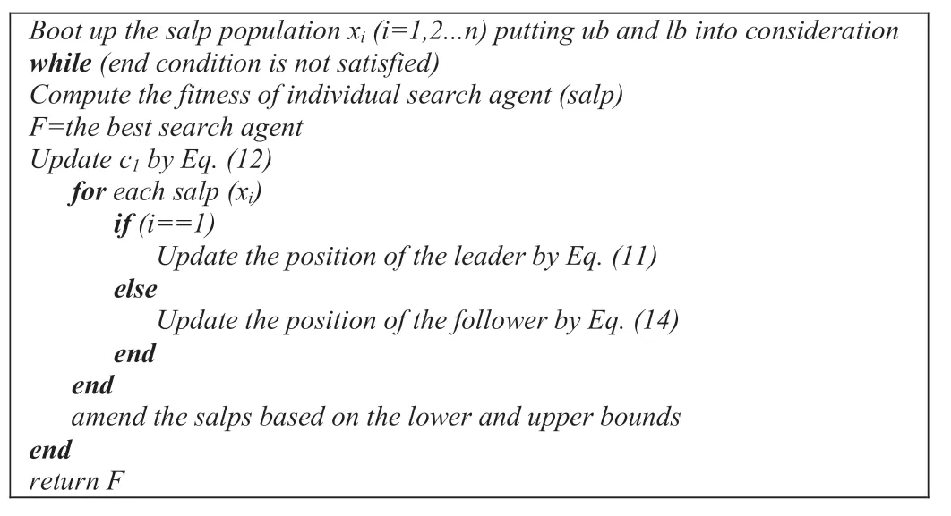
Fig.3.Pseudo-code for the SSA proposed by Mirjalili et al.(2017).
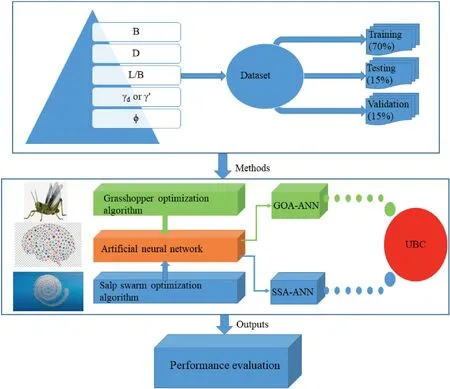
Fig.4.Schematic diagram of model procedures.

Fig.5.Optimum 5-8-1 ANN structure adopted.
where γ*is either γdor γ'as denoted in the adopted database.
Similarly, the obtained UBCSSA-ANNmathematical form is presented as
where xi(i = 1, 2,…,8)is given below using the weights and b1in Table 3:
It should however be noted that the coefficients of the independent variables B, D, L/B, γ*and φ and the constants in y1to y8and x1to x8are supposed to be the same as the weights and biases in Table 3, but some mathematical manipulations have been performed to simplify them to avoid the need for the pre-processed(or normalized) datasets.This is necessary because the independent variables are in the normalized form as required by the ANN.Then,to obtain the presented y1to y8and x1to x8, each of the modelindependent variables is respectively replaced with (2B-3.0745)/2.9575, (2D-0.889)/0.889, (2L/B-7)/5, (2γ*-26.95)/7.25, and(2φ-76.8)/12, as obtained using Eq.(15).

Table 3Weights and biases used for developing the mathematical models.
3.Results and discussion
3.1.Performance evaluation
The performance of the proposed models was evaluated using four statistical indices as adopted by Patmini et al.(2008)together with the same number of datasets used for the calibration and validation in their model.The coefficient of correlation (R), coefficient of efficiency (E), RMSE, and MBE between the proposed models and the measured values are respectively determined as follows:
where ymistands for the measured UBC;yciis the predicted UBC;μmyand μcyare the means of the measured and predicted UBCs,respectively; and n is the number of data points.Fig.6 shows the correlation between the predicted and measured UBCs for the calibration and validation datasets.The ideal fit lines together with±5% error lines are also included in Fig.6.It can be seen that the predictions of GOA-ANN and SSA-ANN models largely fall within the defined error lines, indicating that the prediction of the proposed models is very close to the ideal lines.Only two points in the calibration results fall closer to the -5% and 5% error lines in the GOA-ANN and SSA-ANN models.The obtained results for the calibration and validation phases indicated that the proposed models are suitable for accurate predictions of the UBC of the shallow foundation.The results obtained using Eqs.(20)-(23) are also presented in Table 4 including that of the ordinary ANN model.The R and E values obtained for the two phases for the ordinary ANN,GOA-ANN, and SSA-ANN are close to 1, which indicates that the proposed models can give reliable predictions of the UBC.The obtained errors for the two phases are low, but that of the ordinary ANN is the highest, most importantly, in the validation phase.The MBE indicates that the ordinary ANN, GOA-ANN, and SSA-ANN models are slightly overestimating the UBC except for the SSAANN model in the calibration phase where the UBC is slightly underestimated.The results of the performance indicators obtained, as presented in Table 4, are better than the existing SC models, most specifically in the validation phase, which is a very important phase as it enables the identification of over- or underfitting of the network.For example, in Padmini et al.(2008), the least RMSE obtained in the validation phase is greater than 50 kPa in all their models, while Kalinli et al.(2011) gave the RMSE of 29 kPa.The RMSE obtained for the ordinary ANN developed in this study is comparable with that of the existing SC models.Thereafter,the proposed hybrid ANN models will be further compared with the existing models in Sections 3.2 and 3.3.

Table 4Performance evaluations of the models.
In addition, the computational effort is important in geotechnical engineering except the statistical accuracy of the model according to Wang et al.(2020b).The proposed models require less computational effort to implement as they have been transformed into simple mathematical forms and the MATLABcode which can effortlessly be used on any computer within a few seconds has been written, as presented in the Appendix A.Therefore, the proposed models are easy to implement practically.
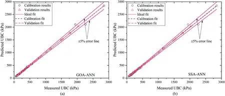
Fig.6.Prediction performance of the GOA-ANN and SSA-ANN models.
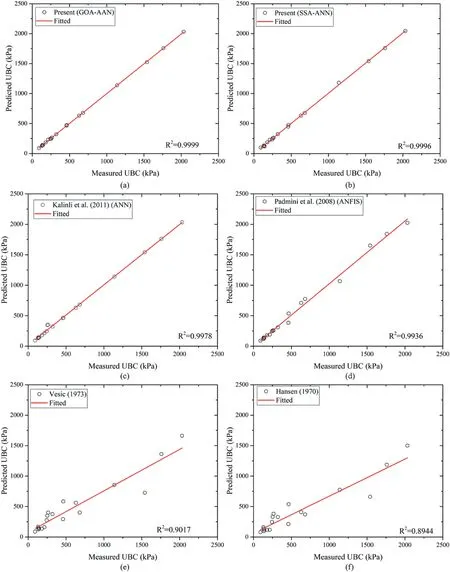
Fig.7.Comparison of the models: (a) GOA-ANN; (b) SSA-ANN; (c) Kalinli et al.(2011); (d) Padmini et al.(2008); (e) Vesic (1973); and (f) Hansen (1970).
3.2.Model comparison
The proposed models for the predictions of UBC of the shallow foundation are compared with the ANN model proposed by Kalinliet al.(2011), the outperforming model among the SC models proposed by Padmini et al.(2008) (i.e.ANFIS model), and theoretical equations presented by Vesic (1973) and Hansen (1970) using the same validation datasets as adopted by Padmini et al.(2008) and Kalinli et al.(2011).Two strategies are used for this comparison.The first strategy is to present the comparisons graphically,as shown in Fig.7,based on the data listed in Table 5,and the second strategy is based on the percentage relative error (RE) criteria adopted by Padmini et al.(2008), which is presented in Table 6.

Table 5The validation datasets adopted by Padmini et al.(2008) and Kalinli et al.(2011).

Table 6Comparison of the proposed models with the existing models using RE and MARE.
The outcome of the first strategy revealed that the proposed GOA-ANN and SSA-ANN models have R2of 0.9999 and 0.9996 while the R2values for the models of Kalinli et al.(2011), Padmini et al.(2008), Vesic (1973) and Hansen (1970) are 0.9978, 0.9936,0.9017, and 0.8944, respectively.The proposed models have the highest R2values than the other existing models, and they arestatistically stable in that their adjusted R2and R2are consistent.Before this study, the ANN model of Kalinli et al.(2011) and the ANFIS model of Padmini et al.(2008) appear to be the most accurate as the performance of the recently published GPR model of Ahmad et al.(2021) based on the same parameters as those adopted by Padmini et al.(2008) and Kalinli et al.(2011) is very poor.In addition, mathematical models are made available in this study for practical implementations of the proposed models,which are lacking in the previous studies.Hence,the proposed study can be said to be the most accurate among the existing models for UBC predictions based on the adopted datasets and it is practically implementable.
For the second strategy, the percentage RE and the mean percentage absolute error (MARE) can be computed:
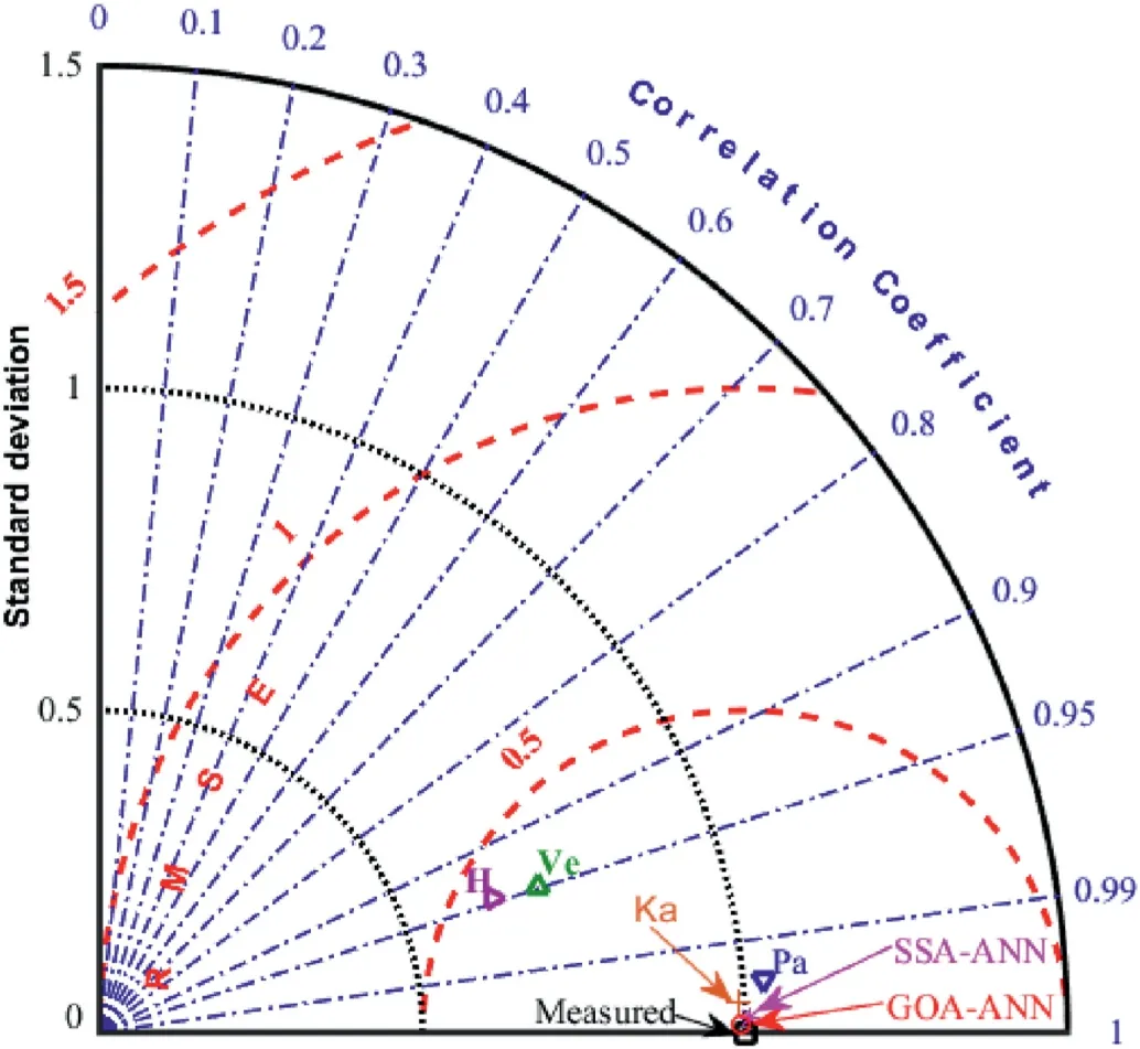
Fig.8.Taylor’s diagram showing the closeness of the proposed models and previous models to the measured values.Ka-Kalinli et al.(2011);Pa-Padmini et al.(2008);Ve-Vesic (1973); H - Hansen (1970).
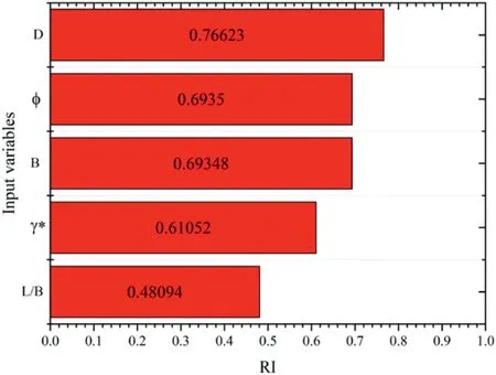
Fig.9.The relative importance of the model variables.
where ymand ycare measured and predicted UBCs, respectively;and n is the number of data points in Table 5.The outcomes of the error comparison with different SC models and commonly used empirical models are presented in Table 6.From Table 6, the RE values of the proposed models are smaller as compared with the other models.As a result,the MARE of the GOA-ANN and SSA-ANN models are 1.54 and 3.22, respectively, which are significantly lower compared with those of the models proposed by Kalinli et al.(2011), Padmini et al.(2008), Vesic (1973), and Hansen (1970),which are 4.09, 6.38, 23.82, and 28.51, respectively.Again, the proposed models have the least RE and MARE values, indicating their abilities to give the closest predictions to the actual values of the UBC.
In addition, AIC is also used to select the best model out of the compared models using the data in Table 5:
where SSE is the sum of squares error,and p is the model predictor variable.The SSE used in Eq.(26)was determined in the OriginPro software.The obtained AIC values for the GOA-ANN,SSA-ANN,and models of Kalinli et al.(2011), Padmini et al.(2008), Vesic (1973),and Hansen (1970) are 73.59, 99.34, 129.18, 151.24, 189.31, and 186.6, respectively.Based on the AIC, the proposed GOA-ANN and SSA-ANN are the best as they have the least AIC values.Therefore,the UBCs of the shallow foundation can be accurately predicted,relying on the proposed SC models in this study.
3.3.Taylor’s diagram
Taylor’s diagram combines three different statistical indicators and employs them to depict the closeness of the models to the measured values.The Taylor’s diagram published by Taylor (2001)is originally used for climate models and earth environmentrelated problems, and recently, it has been used by various researchers in different fields (Lawal et al., 2021a).It has also been used in this study to enable easy understanding or selection of the best models out of the compared models.It can be seen from Fig.8 that GOA-ANN and SSA-ANN are the closest to the measured value,followed by the models of Kalinli et al.(2011),Padmini et al.(2008),Vesic (1973), and Hansen (1970).This implies that the proposed GOA-ANN and SSA-ANN have the highest coefficient of correlation(R) and lowest STD and RMSE values.Hence, they are suitable for predicting the UBC of shallow foundations.
3.4.Relative importance analysis
The relative importance of the various input variables used in developing the models is computed in this study using the cosine amplitude method (CAM) (Yang and Zhang, 1997).Jong and Lee(2004) illustrated that the CAM is suitable for assessing the relative importance of the model variables,and it has been widely used in previous studies on machine learning according to Ahmad et al.(2021).The mathematical expression for CAM is presented as
where RI is the relative importance of each input variable, Iiis the input variable, Miis the model output, and n is the number of trained data points.The outcome of the relative importance analysis conducted based on the GOA-ANN model, which is the most accurate among the proposed models, is presented in Fig.9.From Fig.9,D appears to be the most important input variable,followed by φ, B, γ, and L/B.The RI values of φ and B are almost the same though that of φ is slightly higher.The studies conducted by Kohestani et al.(2017)and Ahmad et al.(2021)also identified D to be the most influencing parameter in UBC prediction.
4.Conclusions
The UBC of soil is imperative in geotechnical/foundation engineering because the load acting on the soil and its competency rely on the bearing capacity.The experimental measurements remain the most reliable means of measuring the UBC.However, this method is very costly and highly time-consuming.The quest for cheap and quick means of measuring or determining the UBC led to the development of models which are largely limit equilibrium based.Nevertheless, there is a huge disparity between the experimental and model results.The suitability of SC for the prediction of UBC has been assessed using the database of the experimental results.The performance of SC models is better and closer to the experimental results than any of the theoretical models.However,the practical implementation of the available SC models is difficult because they are not expressed in the form of mathematical equations.In addition, the error associated with the validations of the existing SC models is also very high.Hence, it is necessary to further explore advanced SC models for possible minimization of the error values.Therefore, GOA-ANN and SSA-ANN are proposed in this study for predicting UBC.The datasets obtained from the existing experimental data of UBC were used for this study.Ordinary ANN was first performed to generate the objective function of the optimization algorithms.Different ANN simulations were performed by varying the number of neurons in the hidden layers.The most accurate ANN architecture was selected and subjected to the adopted optimization algorithms.The models were developed and implemented in the MATLAB environment.The performance of the proposed models was evaluated using the coefficient of correlation(R), RMSE, percentage RE, and MARE.The conclusions delineated below can be drawn from the output of the study:
(1) The proposed GOA-ANN and SSA-ANN have a coefficient of correlation and coefficient of determination that are close to 1.
(2) The obtained MARE is 1.54 for the GOA-ANN and 3.22 for the SSA-ANN.These are the lowest values of MARE among the existing models.
(3) The proposed models have a very low standard deviation from the measured UBC as revealed by Taylor’s diagram.
(4) The mathematical models proposed serve as useful tools for cheap, quick, and accurate estimation of the UBC.
(5) The proposed models will perform very well for the range of the datasets used in developing the models just like any other models including AI/SC-based models.In addition,the models are limited to cohesionless soil scenarios.
Finally, the proposed models are the most accurate SC models compared with the existing SC and theoretical models based on the adopted database and therefore recommended for reliable estimations of the UBC.
Declaration of competing interest
The authors declare that they have no known competing financial interests or personal relationships that could have appeared to influence the work reported in this paper.
Acknowledgments
This work was supported by Korea Research Fellowship Program through the National Research Foundation of Korea(NRF)funded by the Ministry of Science and ICT(Grant No.2019H1D3A1A01102993)and the Inha University Research Grant(2022).
Appendix A.Supplementary data
Supplementary data to this article can be found online at https://doi.org/10.1016/j.jrmge.2022.04.005.
 Journal of Rock Mechanics and Geotechnical Engineering2023年3期
- Journal of Rock Mechanics and Geotechnical Engineering的其它文章
- Long-term decay of the water pressure in the osmotic tensiometer
- Effects of intermediate stress on deep rock strainbursts under true triaxial stresses
- A post-peak dilatancy model for soft rock and its application in deep tunnel excavation
- Numerical simulation of fatigue crack propagation in heterogeneous geomaterials under varied loads using displacement discontinuity method
- Combined load bearing capacity of rigid piles embedded in a crossanisotropic clay deposit using 3D finite element lower bound
- Predicting and validating the load-settlement behavior of large-scale geosynthetic-reinforced soil abutments using hybrid intelligent modeling
