Allometry-based estimation of forest aboveground biomass combining LiDAR canopy height attributes and optical spectral indexes

Qiuli Yang,Yanjun Su,Tianyu Hu,Shihao Jin,Xiaoqiang Liu,Chunyue Niu,Zhonghua Liu,Maggi Kelly,Jianxin Wei,Qinghua Guo

Keywords:Forest aboveground biomass Drone LiDAR Allometric relationship Power law Tree height Vegetation index

A B S T R A C T

1.Introduction

Forest ecosystems represent the largest terrestrial carbon stock and an important carbon sink(Pan et al.,2011;Piao et al.,2009).Accurately quantifying forest aboveground biomass(AGB),an important component of forest carbon storage,has long been an essential task of forest management and protection(Houghton,2005;Pan et al.,2013;Zhao et al.,2012).Traditionally,forest AGB has been measured through field harvest or in situ allometric equation-based methods(Chave et al.,2005;Ningthoujam et al.,2018).Although the field harvest method is highly accurate,it is destructive and is not suitable for spatially continuous AGB estimations(Viana et al.,2012).The allometric equation-based method uses empirical exponential regression equations derived between harvested AGB measurements and forest inventory attributes(Chen,2015)that are then applied to feasible-to-measure tree attributes such as tree species,diameter at breast height(DBH),and tree height.The allometric equation-based method is highly accurate(R2>0.9)(Luo et al.,2019;Paul et al.,2016)but relies on very time-consuming and labor-intensive field inventory information collections.How to improve the efficiency and accuracy of spatially continuous forest AGB estimation is still an active field of research.

Over the last three decades,the rapid development of various remote sensing technologies provides a more efficient technical means for collecting spatially continuous and consistent vegetation observations at multiple scales(Galidaki et al.,2017).Satellite images have been widely used in estimating forest AGB through the aid of field AGB estimations across multiple spatial scales(Tan et al.,2007).Since remote sensing images cannot directly provide forest AGB estimates,these studies usually built a regression model between field AGB estimates and remote sensing indices(e.g.,normalized difference vegetation index/NDVI)to provide spatially continuous forest AGB(Pandey et al.,2019;Xiao et al.,2019).However,the accuracy of forest AGB estimates using this approach can be limited to 10%–50%depending on the forest type(Lu,2007)and may suffer from saturation effects(Huang et al.,2015).Although optical images can capture the spectral heterogeneity of forest stands with different species compositions,they cannot penetrate tree canopies and thus do not provide forest vertical structure information,which may lead to high estimation uncertainty in areas with dense and multi-layered canopies(Mitchard,2018).Recent advances in near-surface remote sensing platforms(e.g.,unmanned aerial vehicle/UAV)have greatly improved the spatial resolution of optical images.However,because they still do not provide forest structure information,their forest AGB estimates remain fraught with uncertainty(Domingo et al.,2019;Zhu et al.,2020).

The emerging light detection and ranging(LiDAR)has been shown to be useful for quantifying forest structural attributes.As an active remote sensing technology,LiDAR emits laser beams that can penetrate forest canopies,the acquired point clouds can be used to accurately estimate tree height,crown size,and other structural attributes(Guo et al.,2020;Jin et al.,2021;Liang et al.,2016).These LiDAR-derived structural attributes(e.g.,tree height)can be used along with field measurements to estimate forest AGB through regression models with much higher accuracy(from 30% to 80% for different forest types)(Li et al.,2015;Zald et al.,2014).However,LiDAR data do not provide the rich spectral information of optical images and thus are of limited use for differentiating tree species compositions(Hill and Thomson,2005;Su et al.,2016).Complex forest stands are usually composed of various tree species differing in wood density,and species-induced uncertainty can account for 25% of the total uncertainty of LiDAR-derived forest AGB(Rodig et al.,2019).

To further improve the accuracy of forest AGB estimation,data fusion strategies of optical imagery and LiDAR data have been proposed.The rapid development of UAV LiDAR systems has significantly reduced the cost of simultaneously obtaining LiDAR data and optical images,improving their accessibility(Hu et al.,2021).The combination of optical imagery and LiDAR data can provide both spectral and structural information,and therefore can improve the estimation accuracy of forest AGB(Almeida et al.,2019;Laurin et al.,2014;Li et al.,2021).For example,Li et al.(2016)and Zhang et al.(2019)reported that the fusion of optical imagery and LiDAR data can improve the forest AGB estimation accuracy by 5%–20%.Nevertheless,these studies are still mainly limited to plantations or pure forests(Pe~na et al.,2018)and optical images and LiDAR data are fused by simply feeding them into regression models(e.g.,linear regression,random forest regression model)(Almeida et al.,2019;Ma et al.,2019a),which usually requires a substantial number of field measurements as inputs to disentangle the correlations between forest AGB and various remote-sensing variables(Zeide,1993).It has been well documented that feeding more variables into regression-based models may not necessarily lead to a higher estimation accuracy(Poorazimy et al.,2020)and,therefore,finding a way to build physically meaningful regression-based models to balance the need for field measurements and the number of remote-sensing predictors has long been a research focus of large-scale forest AGB estimation.

Theoretically,the metabolic rate and many other scale-related attributes of a tree follow a power-law formulation known as the West,Brown&Enquist theory(Brown et al.,2004;West et al.,1999;Deng et al.,2020;Enquist et al.,1999).Furthermore,the allometric model with biological laws which uses field biomass and scale-related attributes of a tree(e.g.,DBH and tree height)to estimate forest AGB(Litton and Boone Kauffman,2008;Pilli et al.,2006;Zianis and Mencuccini,2004;Chave et al.,2014).With the recent development of LiDAR technology,especially the launch of new spaceborne LiDAR systems(e.g.,the Global Ecosystem Dynamics Investigation on board the International Space Station and the Advanced Topographic Laser Altimeter System onboard the Ice,Cloud,and Land Elevation Satellite-2),height-related attributes have become more accessible but DBH is still difficult to obtain on a large spatial scale(Guo et al.,2020;Wulder et al.,2012;Xiao et al.,2019).Essentially,DBH is an attribute representing the constant non-reversible feature of tree growth,which is related to the metabolic rate of a tree(Sarrus and Rameaux,1839).Spectral information derived from satellite remote sensing imagery,especially from bands within the red edge portion of the spectrum,has shown a strong capability to estimate vegetation chlorophyll concentration and photosynthetic rate,which are also important indicators of plant metabolic rate(Anjum et al.,2011;Gamon et al.,1995;Reich et al.,2006).Therefore,we hypothesized that a combination of height-related attributes with remotely sensed spectral information through allometric relationships might provide a solution to accurately estimate forest AGB on a large spatial scale with fewer field measurements.

In this study,we aim to develop a forest estimation method through the fusion of forest structure attributes and spectral information using the allometric relationship hypothesized above.To evaluate the proposed method,we collected in situ forest AGB measurements and UAV LiDAR data for 1,370 forest plots across a large latitudinal gradient,covering four typical forest types of China.Moreover,we further compared the effectiveness of the proposed method with other machine learning-based regression methods.We believe that the proposed approach can guide future forest AGB mapping practices,especially through the fusion of new spaceborne LiDAR data and satellite images.

2.Data and methods

2.1.Field measurements

We selected nine study sites over a large latitudinal gradient(21°N-50°N)in China,including three temperate needleleaf-broadleaf mixed forest sites(sites 1–3),two planted temperate coniferous forest sites(sites 4 and 5),three subtropical evergreen broadleaf forest sites(sites 6–8),and one tropical monsoon forest-rainforest(site 9)(Fig.1).The size of each site varied from 30 to 1,082 ha with an average of 500 ha.These sites are covered by a large variety of climate,terrain,and vegetation conditions(Table 1),which ensures the representativeness of the proposed forest AGB estimation method.

Table 1Summary of climate,terrain,and vegetation conditions of the nine study sites.

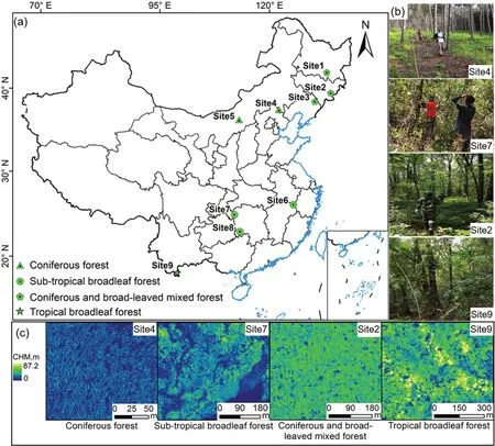
Fig.1.(a)Spatial distribution of study sites and their corresponding forest types,and(b)photos of forest conditions and(c)canopy height model(CHM)in site 4(coniferous forest),site 7(sub-tropical broadleaf forest),site 2(coniferous and broad-leaved mixed forest),and site 9(tropical broadleaf forest).

Within these study sites,we collected 1,370 field plot measurements from 2012 to 2019.Sites 1,3–5,and 7–8 were sampled randomly,and sites 2,6,and 9 were surveyed using a regular sampling strategy(Su et al.,2016).Each study site had at least 20 plots.The size of each plot was 20 m×20 m,except for the 40 plots in site 1(circular plots with a radius of 15 m)and the 30 plots in site 3(30 m×30 m squared plots).Within each plot,we recorded species information of each tree with a DBH greater than 5 cm and measured its DBH and tree height using a diameter tape and a Haglof laser rangefinder(Hagl¨of Sweden,Långsele,V¨asternorrland,Sverige),respectively(Fig.2).For square plots,the location of the plot center and four corners was recorded;for circular plots,we only measured the location of the plot center.Among them,sites 4,5,77,,and 8 were surveyed in 2019,and plot locations were measured by a Global Navigation Satellite System receiver with the support of Qianxun Continuously Operating Reference Stations(h(htttpts:ps://www.qxwz.com/),which can provide a decimeter-level positioning accuracy.Sites 1–3,site 6,and site 9 were surveyed in 2015–2018,and their plot locations were measured by a Trimble Geo 7X.Then,the AGB of each tree was estimated using a species-specific allometric equation provided by Zhou et al.(2018)and Luo et al.(2019).For trees that did not have available allometric equations(accounting for less than 10% of the total number of trees),we used the allometric equations of the dominant tree species in the corresponding plots to estimate their AGB(Zhou et al.,2018).Finally,the total AGB of each plot was estimated by adding up the AGB of all individual trees within it and was used as the ground truth in the following analysis.

2.2.UAV LiDAR data

Within each study site,we collected UAV LiDAR data using a LiAir UAV LiDAR system(GreenValley International Incorporation,Beijing,China)equipped with a RIEGL VUX-1 UAV laser scanner(RIEGL Laser Measurement Systems,Horn,Austria).This LiDAR system was operated at about 200–300 m above ground level with a 400 kHz pulse repetition frequency(Table 2).The flight speed was 8 m⋅s–1,which has proven that can support the acquisition of high-quality LiDAR point cloud data in various forested conditions(Hu et al.,2021).In this study,all collected UAV LiDAR data had a point density higher than 10 points⋅m–2,and can be used to accurately capture the vertical structure of forest canopies in all nine study sites.

Table 2Summary of flight and scanner parameters used for collecting UAV lidar data in the nine study sites.

All collected UAV LiDAR data were preprocessed with the LiDAR360 software(GreenValley International)following the procedure suggested by Guo et al.(2018),including strip alignment,outlier removal,filtering,and canopy height extraction(Fig.2).Strip alignment is used to adjust the systematic misalignment of point clouds from different UAV flight strips,and outlier removal is used to remove random errors caused by flying objects or multipath effects.Filtering aims to identify ground points from LiDAR point clouds.We used an improved progressive triangulated irregular network densification filtering algorithm implemented in the LiDAR360 software to extract ground points(Zhao et al.,2016).Finally,the extracted ground points and the highest non-ground points were interpolated into a 1-m resolution digital terrain model(DTM)and digital surface model(DSM)using the ordinary kriging method(Guo et al.,2010),and the canopy height model(CHM)was calculated as the difference between DSM and DTM(Fig.2).

For each study site,we collected a single-scene Level-1C Sentinel-2 image from the Copernicus Open Access Hub to derive vegetation indices.All images were collected during the growing season(from July to October)of 2019 or 2018 without cloud coverage,except for site 9.Site 9 is a tropical monsoon forest-rainforest and here cloud-free images are hard to acquire during the growing season.Therefore,we selected an image from March 2019 as an alternative(Table 3).Then radiometric calibration and atmospheric correction were conducted to acquire the Level-2A images using the Sen2Cor tool(http://step.esa.int/main/th thiirrdd-partyplugins-2/sen2cor/),which transformed top-of-atmosphere reflectance to land surface reflectance.Since the normalized difference vegetation index(NDVI)has been widely used for forest biomass estimation and has been shown to be an effective indicator,here we calculated NDVI from the red band(665 nm)and near-infrared band(842 nm)of the Level-2A images at 10 m resolution as an indicator of spectral information in the forest AGB modeling.

2.3.Optical images

2.4.Structural and spectral features extraction

Four canopy height-related metrics and four spectral metrics were extracted from the collected UAV LiDAR data and Sentinel 2 images(Fig.2),including maximum height(THmax),mean height(THmean),the standard deviation of canopy height(THstd),and coefficient of variation of canopy height(THcv),maximum NDVI(NDVImax),mean NDVI(NDVImean),the standard deviation of NDVI(NDVIstd),and coefficient of variation of NDVI(NDVIcv)(Table 4).Among the four canopy height-related metrics,THmax,THmean,THstd,and THcvwere calculated as the maximum,mean,standard deviation,and coefficient of variation of all 1-m CHM pixels within each plot.These attributes represent the vertical distribution of the canopy(THmaxand THmean)and provide insights into the vertical complexity and heterogeneity(THstdand THcv)of the canopy components(Li et al.,2016).

Table 3Description of the collected Sentinel-2 images.

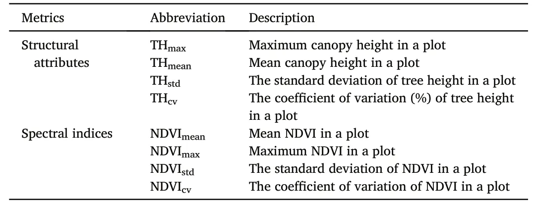
Table 4Descriptions of canopy height-related metrics and spectral metrics extracted from UAV LiDAR data and Sentinel-2 images.

Four spectral metrics were calculated from the NDVI using the zonal statistic tool in the ArcGIS Pro software(Esri,Inc.).The spatial resolution of the extracted structural and spectral metrics was consistent with the plot size in each study site,except in site 1,where circular plots with a radius of 15 m were approximated by 30 m×30 m plots.

Owing to the heterogeneity of forest stands,the optimal structure and spectral variables differ across study sites.Before assessing the predictability of canopy height-related metrics and vegetation index-related metrics,simple regression models were implemented to test the ability of each variable to predict biomass in the nine study sites.Models with the highest coefficient of determination were treated as the best models,and their corresponding independent variables were selected as the best metrics.To construct a universal and robust model that is suitable for different forest types and stand characteristics,we first chose typical and representative study sites.Then,we selected the metrics with optimal linear correlation with AGB and the highest cumulative determination coefficient(R2)among the study sites of different forest conditions for the subsequent biomass model building and verification.

2.5.The proposed biomass retrieval method

Conventionally,an allometric relationship establishes a model between feasible-to-measure tree attributes(e.g.,DBH)and forest AGB using a power-law formulation(West et al.,1997,1999).The ratio of relative growth rates is recognized as a constant(Huxley and Teissier,1936),which varies slightly with species and growing environment.At present,however,the constant in the law has been challenged by many forest ecosystem studies(Poorter et al.,2015;Zhou et al.,2021;West et al.,2009).Furthermore,Asner and Mascaro(2014)used regional-scale inputs of basal area and wood density to link tropical forest field biomass and LiDAR top-of-canopy height.Here we focused on the allometric relationship at the plot level instead of single trees,hoping to reduce the cumulative error caused by the biomass estimation error of a single tree.In a forest plot or landscape,we hypothesized that the allometric relationship also exists between the easily-measured forest attributes and biomass.Given that canopy height is easier to obtain than the DBH and the vegetation index can reflect the heterogeneity of the crown and the metabolic rate of the species,we propose an approach that uses a vegetation index VI variable as the power of a canopy height TH variable to build a physically meaningful regression model for forest biomass retrieval.The specific form of the proposed biomass estimate method follows Equation(1)and it can be linearized by calculating the logarithms as in Equation(2).

where TH is a canopy height metric in each plot,VI is the vegetation index in each plot,andaandbare parameters.

Previous studies coupled structural metrics and spectral indices as separate input features,so-called feature-level data fusion,for biomass estimation(Li et al.,2016;Tilly et al.,2015).The proposed approach incorporates optimal structural and spectral metrics as a single feature VI×log(TH)was trained using linear regression.Because there were mismatches in data acquisition time between field measurements and UAV lidar data,we used the following criteria to filter field measurements.1)Complete field inventory records should be measured,including plot location,species,tree height,and DBH;and 2)plots should not fall on the edge of UAV lidar data.After data filtering,1,250 plots were used to evaluate the performance of the proposed forest AGB estimation method in all sites across coniferous forest,sub-tropical broadleaf forest,coniferous and broadleaf-leaved mixed forest,and tropical broadleaf forest.In all sites and forest types,70% of the plots were randomly selected for training and 30% for testing.Two statistical measures–coefficient of determination(R2)and root-mean-squared error(RMSE)–were calculated as follows:

wherenis the number of testing plots;yiand^yirepresent the field and predicted AGB in ploti,respectively;yiis the mean of field AGB.

2.6.Comparison with existing methods

We further compared the calculation of AGB of the nine study sites of the proposed method with current commonly-used machine learningbased regression methods,including multilinear regression(SMR),artificial neural network(ANN),and random forest(RF).To be consistent with the proposed method,these three machine learning regression models were also trained and tested using the same field measurements plots.The three machine learning regression models were implemented using all TH and VI metrics as input variables in the R package caret(Kuhn,2008).

Data uncertainty and model robustness are among the most important challenges for ecological modeling studies.To ensure that the model accuracy was not affected by the distribution of certain test samples,and the prediction accuracy of different models was comparable,we first run the model under different sample sizes(from 10 to 100 plots)to evaluate the performance of our proposed approach and the RF model.Secondly,for each sample size,the experiment was repeated ten times with randomly selected plots from 1,250 plots and corresponding forest types.The trained and tested data used by the two methods were the same in each experiment.Then,the average and standard deviation of theR2and RMSE in ten experiments between predicted and field AGB were calculated.

3.Results

3.1.The selection of structural and spectral indexes for forest AGB estimation

For structural attributes,THmeanperformed the best in all sites in terms ofR2between predicted and measured AGB(Fig.3).The modeling accuracy of THmax,THcv,and THstdvaried with forest type.Among them,THmeanand THmax,which represented the vertical distribution of canopy height,had the greatest contributions to the model performance of coniferous forest(site 4 and site 5)and sub-tropical broadleaf forest(site 6,site 7,and site 8).THcvand THstd,which can provide insights into the vertical complexity and heterogeneity of the canopy components,performed the best in coniferous and broad-leaved mixed forests(site 1,site 2,and site 3).

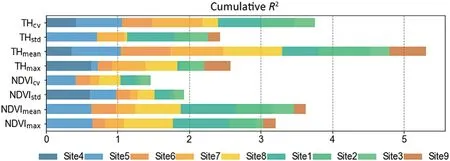
Fig.3.Stacked bar plots of the R2 values from simple regression models based on different metrics in all study sites.

The vegetation index NDVImeanperformed the best in all sites(Fig.3).The lowR2(<0.1)values of NDVIcvand NDVIstdat site 9 implies that the spectral heterogeneity of forest canopies was small in tropical broadleaf forest(site 9)with ultra-high biomass.Besides,NDVImax(R2=0.18)and NDVImean(R2=0.17)also had almost no difference in response to biomass in tropical broadleaf forest,and theR2of both was relatively low.However,the highR2values at sites 6–8 and sites 1–3 indicate they were sensitive to the AGB in sub-tropical broadleaf forest and coniferous and broadleaf-leaved mixed forest.

As THmeanand NDVImeanachieved the best overall performance among all TH-metrics and VI-metrics in 9 sites,they were adopted in the proposed method(Fig.3).Furthermore,we presented the probability density distributions of field-measured AGB and selected metrics(THmeanand NDVImean)with respect to each forest type(Fig.4).Forest AGB,THmean,and NDVImeanmetrics in sub-tropical broadleaf forest,coniferous and broadleaf-leaved mixed forest,and tropical broadleaf forest presented a normal distribution,except in coniferous forest(the stand density at site 5 was very low).In addition,AGB and THmeanshowed a substantial gradient among different forest types.Because most sites belong to mature forests,the value range of NDVImeanwas relatively narrow.Nonetheless,the distribution of AGB(3.58–850 Mg⋅ha–1),NDVImean(0.47–0.86),and THmean(1.5–50 m)demonstrate that the selected plots well represented different forest conditions.

3.2.The performance of the proposed approach

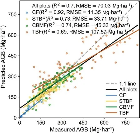
Fig.5.Measured and predicted AGB from the proposed method for all plots and different forest types.Note that CF represents coniferous forest,STBF represents sub-tropical broadleaf forest,CBMF represents coniferous and broadleaf-leaved mixed forest,and TBF represents tropical broadleaf forest.

This study demonstrated a new method for forest AGB estimation that combines vertical structure attributes of LiDAR point clouds with canopy surface spectral information of Sentinel-2.As shown in Fig.5,our proposed biomass modeling method achieved good prediction accuracy in all plots and different forest types.The forest type-based modeling was found to be more accurate than using all sample plots.Our approach showed the highestR2=0.92 and lowest RMSE=11.35 Mg⋅ha–1in coniferous forest,followed by coniferous and broadleaf-leaved mixed forest(R2=0.74,RMSE=45.33 Mg⋅ha–1),sub-tropical broadleaf forest(R2=0.73,RMSE=33.71 Mg⋅ha–1),and tropical broadleaf forest(R2=0.69,RMSE=107.57 Mg⋅ha–1).Secondly,the data distribution of predicted and measured biomass was modulated in coniferous forest,subtropical broadleaf forest,and coniferous and broadleaf-leaved mixed forest,and they were both around the 1:1 line.In tropical broadleaf forest,the proposed method also did not cause large overestimation and underestimation in low and high biomass areas,respectively.

The proposed method using THmeanand NDVImeanfor each forest type(Table 5)was then applied to map the AGB at the nine study sites with a 20-m spatial resolution(Fig.6).The average biomass of the three sites in the coniferous and broadleaf-leaved mixed forest was relatively high(greater than 180 Mg⋅ha–1).Secondly,the average biomass of the tropical broadleaf forest was 203.61 Mg⋅ha–1,and the biomass of site 7 in the subtropical broadleaf forest was 115.41 Mg⋅ha–1.Furthermore,site 5 in the coniferous forest belongs to the temperate steppe vegetation zone.The dominant speciesPinus tabuliformisandUlmus davidianawere short and small,and the canopy cover was usually lower than 0.5(Table 1),which resulted in low average biomass of 6.78 Mg⋅ha–1.In addition,it can be seen from Fig.6 that our method was sensitive to low(Fig.6e)and high biomass(Fig.6a,b,c,and i).

Fig.4.Data distribution of(a)field biomass(AGB),(b)spectral indices(NDVImean),and(c)structural attributes(THmean)in different forest types.Note that CF represents coniferous forest,STBF represents sub-tropical broadleaf forest,CBMF represents coniferous and broadleaf-leaved mixed forest,and TBF represents tropical broadleaf forest.

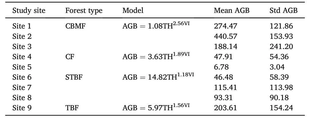
Table 5The summary of AGB mapping at the nine study sites.

3.3.Comparison with existing methods

Compared with approaches using only structural or spectral information,the proposed approach using TH metrics or VI metrics for biomass estimation that combined NDVImeanand THmeanhad a better performance in terms of theR2and RMSE between predicted and field AGB(Fig.7d–f and Table 6).The addition of the spectral index(NDVImean)improved the prediction ability of models solely on THmean,especially in the coniferous and broadleaf-leaved mixed forest where theR2increased from 0.67 to 0.74 and RMSE significantly decreased by 14%(Fig.7e and f).For all data,our model still achieved a better accuracy,withR2=0.70 and RMSE=70.03 MMgg/.hhaa–,1than the model based on TH,with R2=0.65 and RMSE=76.49 Mg⋅ha–1.In addition,there was a strong saturation of the optical image in high biomass areas(biomass>300 Mg⋅ha–1)(Fig.7a–c),but the distribution of the points was more compact when fusing structural information(Fig.7f).In general,using spectral data as auxiliary information can increase the predictive ability of biomass by about 10%(Table 6).

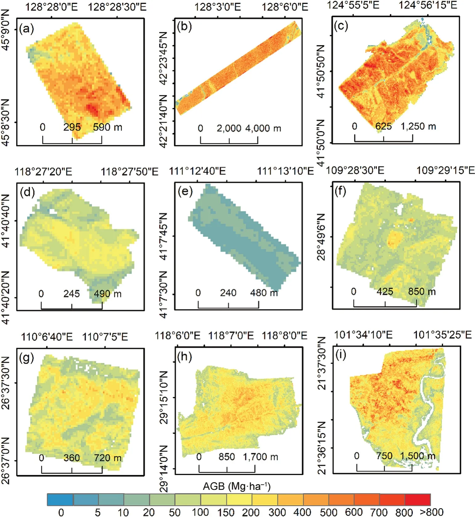
Fig.6.Spatial variability of AGB prediction from the proposed method.a–i represent sites 1–9,respectively.

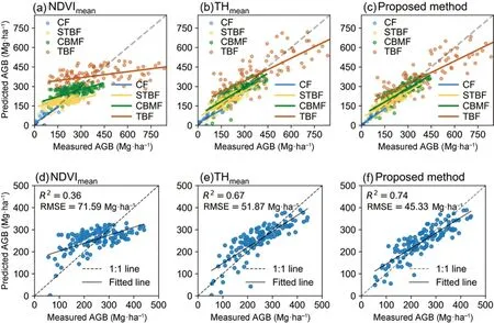
Fig.7.Comparisons between measured AGB and predicted AGB by using different model scenarios.a:only NDVImean data,b:only THmean data,and c:combining NDVImean with THmean using the proposed method.d–f were a–c in CBMF,respectively.

To further assess the capability of the proposed method,three advanced machine learning models were employed and tested.In different forest types,SMR,ANN,and RF provide different advantages(Table 6 and Fig.8a–c).Taking coniferous and broadleaf-leaved mixed forest as an example,RF performed the best withR2=0.70 and RMSE=61.63 Mg⋅ha–1,followed by ANN and SMR(Fig.8d–f).For SMR and RF models,two of the three most important variables were THmeanand NDVImean(Fig.8g and i).For the ANN model,the two most important variables were THcvand NDVImax.However,the proposed method with simple linear regression outperformed statistically multivariate machine learning-based regression models SMR,ANN,and RF,even though all the TH-and VI-metrics were used to predict AGB while the proposed method only required THmeanand NDVImean(Table 6).This indicates that our method was feasible and captured the changes in biomass.Furthermore,in the proposed method,only two variables were used as predictors,which was computationally simple and efficient compared to machine learning-based regression models.These results emphasized the potential of our method as an efficient and accurate indicator for large-scale biomass estimation,such as in the context of China's carbon-neutral plan.

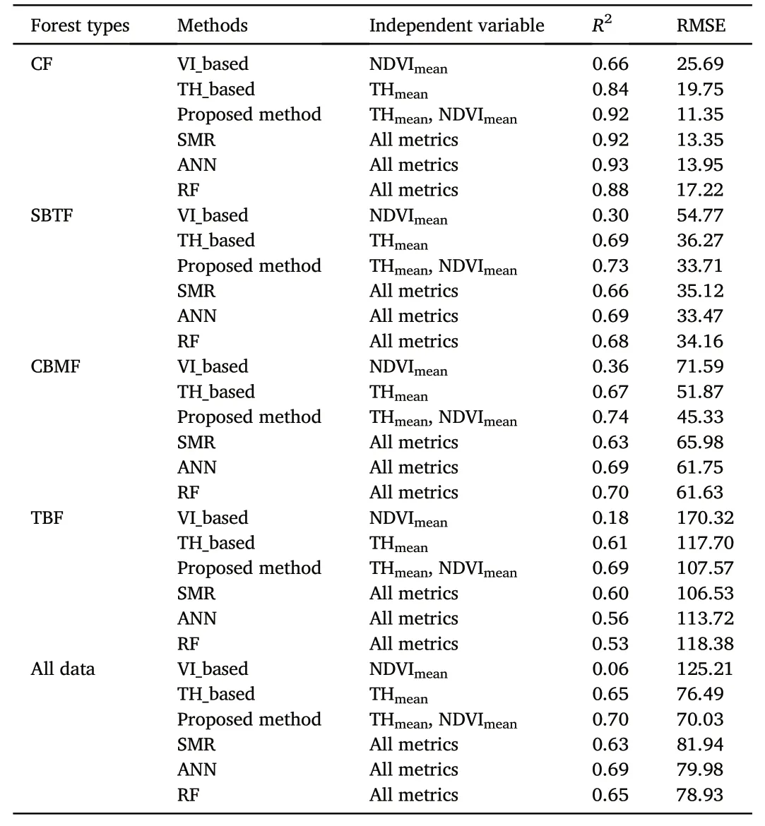
Table 6Validation statistics for AGB estimation using the proposed method for different forest types.

3.4.The effect of sample size on method performance

Overall,our results showed that the accuracy of the proposed method was stable with an averageR2of about 0.7 and RMSE of about 85 Mg⋅ha–1from 10 to 100 plots(Fig.9).However,the accuracy of RF showed an increasing trend with a sample size of fewer than 40 plots and then stabilized with the increase of samples;the standard deviation ofR2or RMSE from the ten experiments also gradually decreased with increasing sample size.In summary,our proposed method outperformed the RF model in terms of bothR2and RMSE.We also conducted experiments in different forest types(Fig.10).Although the performance was slightly different in the four forest types,our model performed very well overall.In sub-tropical broadleaf forest and tropical broadleaf forest,our model performed better in small sample sizes and was still slightly better than RF in large samples.Although in coniferous forest and coniferous and broadleaf-leaved mixed forest,the meanR2and RMSE of our method were similar to those of the RF model,the standard deviation ofR2and RMSE in our model was more stable and smaller than those of the RF model.

In general,the proposed method had a greater advantage when the sample size was less than 40 plots,and the model still had slightly better accuracy than RF as the sample size increased to 100 plots.This was sufficient to show that our method can be used for forest biomass estimation,especially in the case of limited data.

4.Discussion

Fig.8.Comparisons between measured AGB and predicted AGB by using complex and multivariable models.a:Stepwise multiple regression(SMR),b:Artificial neural network regression(ANN),and c:Random forests regression(RF),d–f were a–c in CBMF and g–i were variable importance of d–f,respectively.

Fig.9.The effect of sample size on the performance of the proposed method and Random Forests(RF)model using all data.The line and errorbar are the mean and standard deviation of RR2 and RMSE from ten experiments with randomly selected plots.

There have always been two challenges in large-scale biomass estimation research:1)simultaneously obtaining large-scale forest structure and spectral information,and 2)the availability of sufficient measurement data(Coops et al.,2021;Guo et al.,2020;Jin et al.,2021;Xiao et al.,2019).In response to these limitations,this study drew on the allometric relationship and used the form of power-law to integrate forest structure and spectral information at the community scale to invert forest biomass at the landscape scale.In the process of model construction,for the structural parameters,we found that THmeanis a better biomass predictor across sites with different forest stand conditions.This is consistent with the results of Zhang et al.(2019).Whether a forest stand is homogeneous,THmeancan reflect the average status of forest structure and growth of the entire forest community(Hawbaker et al.,2009;Li et al.,2015).In addition,the spectral index NDVImeanperforms the best in different sites,which generally aligns with results found in other biomass estimation studies(Campos et al.,2021;Formica et al.,2017;Kumar et al.,2020).Similarly,Raynolds et al.(2006)found that NDVImeancan capture species distribution and growth information in forest communities.Another possible reason is that the average value of NDVI made it less affected by sensor and acquisition time(Gonz′alez-Alonso et al.,2006).

By using optimal structural and spectral metrics,our method achieved good results with R2reaching about 0.7.However,the model differs slightly among forest types,and R2varies between 0.7 and 0.92,which is mainly affected by the two input parameters of the proposed method.Although THmeanreflects the average forest status of the plot,wood density differs among tree species(Baker et al.,2004),especially in heterogeneous forests,causing the variability in the degree of uncertainty in different forest types(Rodig et al.,2019).Second,it can be seen from Fig.5 and Table 6 that the degree of saturation of NDVI differs among different forest types,and the saturation effect is the most serious in rain forests(Gamon et al.,1995).By including THmean,our proposed method can significantly reduce the saturation effect in forest AGB estimation through all forest types(Fig.7).

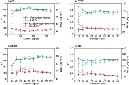
Fig.10.The effect of sample size on the performance of the proposed method and Random Forests(RF)model in different forest types.The line and errorbar are the mean and standard deviation of ten times model accuracy.

Although it is difficult to accurately capture the changes in forest biomass using structural and spectral information alone for forest stands with complex structures,our proposed modeling method increases the biomass estimation accuracy by about 10%.This is mainly due to the contribution of the Sentinel-2 images,which provide information on the spectral heterogeneity of canopies,and can reflect the diversity in stem biomass of forest communities(Huang et al.,2019;Williams et al.,2021).Although TH-related metrics can be obtained from UAV LiDAR point clouds with comparable accuracy to field measurements,they can only explain about¾of the variation in AGB and around¼is species-induced uncertainty(Rodig et al.,2019).Our results also confirmed that the species-induced ambiguities can be reduced(~10%)by deriving vegetation index from high-resolution spatial and spectral measurements(Fig.7 and Table 6).It has been reported that combining structural and reflectance spectral metrics can improve the accuracy of AGB predictions in agricultural and grassland ecosystems(Almeida et al.,2019;Ma et al.,2019a;Maimaitijiang et al.,2019;Martin et al.,2012),as well as in planted forests(Pe~na et al.,2018).Our approach also works well for forest ecosystems with complex forest stands and high AGB(Fig.6i).

In addition,compared with machine learning-based regression methods(SMR,ANN,and RF),our method has higher accuracy for biomass inversion(Fig.8).This indicates the allometric relationship built from forest structural attributes and remotely sensed spectral information is an alternative method for large-scale forest AGB estimation.Although RF is a non-parametric method,it integrates the advantages of a large number of decision trees to improve estimation accuracy.However,the presence of more noise and features increases the likelihood of incorrect decisions in the random forest model(Belgiu and Dr˘agut¸,2016).More input features do not guarantee better performance in AGB prediction under different forest types and stand characteristics.Thus,combining laser scanning data,spaceborne radar data,and digital aerial imagery to predict biomass may not be necessarily better than just using laser scanning data and space-borne radar data(Poorazimy et al.,2020).

Furthermore,compared with random forest,our method is less sensitive to sample size and is very robust.On the one hand,it is maybe beneficial from using linear regression to invert biomass as it requires a small sample size as input.On the other hand,this also demonstrates that our method has ecological and physical significance.The approach can be used to explore the relationship between tree metabolism and biomass(McMahon et al.,2010;Muller-Landau et al.2006a,2006b)by combining structural and spectral information(Oliveras et al.,2014;Schlund et al.,2018),and this relationship may be more stable in similar landscapes.Additionally,the proposed method can be seen as a geometric model(Picard et al.,2015).When we regard the forest scene as a cube,the change in NDVI can reflect the change in the composition of the material in the cube to some extent(Chave et al.,2005;Maimaitijiang et al.,2019).

The proposed method is simple and robust,providing a new way to precisely derive large-scale forest biomass and ultimately serve China's carbon neutrality goal(Yang et al.,2021).The recently launched spaceborne LiDAR missions(GEDI and ICEsat-2)provide nearly global coverage,evenly distributed,and high-density ground sampling footprints,which can be used to obtain canopy height.In addition,existing optical remote sensing satellites such as Sentinel-2 and the upcoming hyperspectral mission(e.g.,EnMAP)can better capture the spectral information of heterogeneous forest canopies(Rodig et al.,2019).In the future,we will try to integrate these new remote sensing technologies with a higher spatial and spectral resolution,different vegetation indices,and space-borne LiDAR for biomass inversion at regional and global scales.

Nevertheless,there are still several limitations in the current study.First,field measurements in this study were obtained at different times with different sizes,which may bring errors to the forest AGB estimation results.Moreover,the limited number and size of plot measurements make us hardly investigate whether there is a scale effect in the allometric relationship built from forest structural attributes and remotely sensed spectral information.Second,although the proposed method does not have a requirement in a large training sample pool,it still has a significant influence on the modeled allometric relationships in different forest types(Table 6).Moreover,as can be seen in Fig.11,if a small training sample pool was used,the estimated coefficients and constants of allometric relationships may vary significantly.However,with the increasing number of plots,their variations become smaller and eventually remain relatively stable after the training sample size reaches a certain value(80 plots in this study).Therefore,we suggest that a relatively large training sample pool should be used for all forest types in large-scale forest AGB estimation practices.

Fig.11.Variations of(a)coefficient and(b)constant using the proposed forest AGB estimation method with different numbers of plots.Each gray dots represent modeled coefficient or constant values using the corresponding number of plots randomly selected from the original training sample pool.

5.Conclusion

This study presented a simple and efficient approach for combining forest structure attributes and spectral indices from UAV LiDAR point clouds and Sentinel-2 images to accurately estimate forest AGB in the nine study sites covering coniferous forest,sub-tropical broadleaf forest,coniferous and broad-leaved mixed forest,and tropical broadleaf forest.The mean canopy height and mean NDVI were found to be the optimal and universal structural and spectral metrics for the AGB estimation in 1,370 plots from the nine sites.The new approach adopted NDVImeanas the power of THmeanand achieved a better performance than models solely based on tree height metrics,withR2between predicted and measured AGB increased by about 10% and the RMSE decreased by about 22% in four forest types.Moreover,the proposed method also achieved a comparable or even better performance than advanced machine learning models such as RF,ANN,and SMR.With UAV LiDAR and TH metrics derived from other platforms,such as space-borne LiDAR,becoming more accessible,the proposed method is expected to be examined and applied at larger scales for high-precision estimation of the forest.

Declaration of competing interest

The authors declare that they have no known competing financial interests or personal relationships that could have appeared to influence the work reported in this paper.

Acknowledgments

This work was supported by the Strategic Priority Research Program of Chinese Academy of Sciences(Grant No.XDA19050401),and the National Natural Science Foundation of China(41871332,31971575,41901358).