Current climate overrides past climate change in explaining multi-site beta diversity of Lauraceae species in China

Ziyn Lio, Youhu Chn, Kiwn Pn, Mohmm A. Dkhil, Kxin Lin,b,Xinglin Tin, Fngying Zhng, Xiogng Wu, Bikrm Pny, Bin Wng,Niklus E. Zimmrmnn, Lin Zhng,＊, Mihl P. Nobis

a CAS Key Laboratory of Mountain Ecological Restoration and Bioresource Utilization &Ecological Restoration and Biodiversity Conservation Key Laboratory of Sichuan Province, Chengdu Institute of Biology, Chinese Academy of Sciences, Chengdu, 610041, China

b University of Chinese Academy of Sciences, Beijing, 100039, China

c Swiss Federal Institute for Forest, Snow and Landscape Research WSL, Zürcherstrasse 111, CH-8903, Birmensdorf, Switzerland

d Botany and Microbiology Department, Faculty of Science, Helwan University, Cairo, 11790, Egypt

e Department of Forest Sciences, University of Helsinki, P.O. Box 27, Helsinki, FI-00014, Finland

f Academy of Agriculture and Forestry, Qinghai University, Xining, 810016, China

Keywords:Biodiversity conservation Current climate Ensemble modelling Multi-site β-diversity Nestedness Past climate change True turnover

ABSTRACT Background: We aimed to characterise the geographical distribution of Sørensen-based multi-site dissimilarity(βsor) and its underlying true turnover (βsim) and nestedness (βsne) components for Chinese Lauraceae and to analyse their relationships to current climate and past climate change.Methods:We used ensembles of small models(ESMs)to map the current distributions of 353 Lauraceae species in China and calculated βsor and its βsim and βsne components.We tested the relationship between βsor,βsne and βsim with current climate and past climate change related predictors using a series of simultaneous autoregressive(SARerr) models.Results: Spatial distribution of βsor of Lauraceae is positively correlated with latitude, showing an inverse relationship to the latitudinal α-diversity (species richness) gradient. High βsor occurs at the boundaries of the warm temperate and subtropical zones and at the Qinghai-Tibet Plateau due to high βsne. The optimized SARerr model explains βsor and βsne well, but not βsim. Current mean annual temperature determines βsor and βsne of Lauraceae more than anomalies and velocities of temperature or precipitation since the Last Glacial Maximum.Conclusions: Current low temperatures and high climatic heterogeneity are the main factors explaining the high multi-site β-diversity of Lauraceae.In contrast to analyses of the β-diversity of entire species assemblages,studies of single plant families can provide complementary insights into the drivers of β-diversity of evolutionarily more narrowly defined entities.

1. Background

Humans are increasingly altering the diversity of life on earth through activities driving climate change, overexploitation of resources, severe pollution,or habitat fragmentation(Gaston,2000;MacDougall et al.,2013;Schluter and Pennell, 2017). To better understand the causes and consequences of global biodiversity loss,we need a deeper understanding of the geographic differences in biodiversity and how this diversity has evolved.Animportant measure of suchdifferencesisβ-diversity,which describesthe differencesin speciescompositionbetween sites(Tuomisto,2010a,2010b).

In contrast to species richness(α-and γ-diversity),β-diversity can be used to analyse species turnover, to map biogeographic units, or to improve networks of protected areas, and it thus has significant and complementary implications in ecology,biogeography and conservation biology (Anderson et al., 2011; Socolar et al., 2016; He et al., 2020).Baselga (2010) proposed that β-diversity can be decomposed into true turnover (species replacement between sites) and nestedness (richness difference between sites).Although this conceptual framework has raised controversies about the ecological interpretation (Chen and Schmera,2015),Baselga's approach(BAS)has been most widely applied over the last decade (reviewed by Soininen et al., 2018). Furthermore, the multi-site version of the β-diversity decomposition framework of BAS(Baselga,2010)is not available in some subsequently published methods,such as the POD (Podani and Schmera, 2011) and SET (Schmera et al.,2020) frameworks.

To date,species richness patterns have often been shown to be related to latitudinal (e.g., Mittelbach et al., 2007) or climate gradients (e.g.,Nobis et al.,2009;Blonder et al.,2018),to differences in soil properties(e.g.,Dakhil et al.,2021),migration limitations(e.g.,Svenning and Skov,2007), human disturbances (e.g., MacDougall et al., 2013) or habitat availability (e.g., Hanski, 2015). In contrast, β-diversity has received much less attention than α- and γ-diversity (Soininen et al., 2018),although there has been a growing interest in β-diversity in community ecology(Condit,2002;Legendre et al.,2009;Wang et al.,2018)as well as biogeography and macroecology (Leprieur et al., 2011; Calatayud et al., 2016; Keil and Chase, 2019; Men′endez-Guerrero et al., 2020).Generally, the β-diversity of species assemblages has been found to be higher in mountainous areas and at biogeographic boundaries (Gaston et al., 2007; Melo et al., 2009). The causes have been attributed to the variation in current climate, either alone or via its interaction with elevation and topographic complexity (Melo et al., 2009). In addition,climate anomalies (Sandel et al., 2011) and velocity of climate change(Loarie et al.,2009)have been used to understand how historical climate change shaped present-day species distributions and assemblies, which may not be captured by current climate only (McFadden et al., 2019;Alahuhta et al., 2020). At the same time, drivers of β-diversity and its components also differ between taxa (Zellweger et al., 2017; McFadden et al., 2019), which adds complexity to the interpretation of large-scale gradients of β-diversity, and this applies especially to our understanding of the true turnover and nestedness components.

Large-scale studies of β-diversity are often based on the aggregated presence(–absence)data in grid cells(Wang et al.,2012a;Pinto-Ledezma et al., 2018). This occurrences-to-grid approach, however, can result in flawed β-diversity calculations in regions with unknown or under-sampled species occurrences. A coarse-resolution extent-to-grid approach has been used in other studies(e.g.,Men′endez-Guerrero et al.,2020),but such range mapping(e.g.,IUCN digital range maps)tends to be imprecise,leaving out well-documented but isolated populations,and likely includes areas within the range boundaries where in fact no populations exist(as criticized by Peterson et al.,2018).A third approach is based on macroecological models that link a large number of measured β-diversity values directly with environmental factors(Viana et al.,2016;Keil and Chase, 2019; He et al., 2020). However, since β-diversity does not respond to environmental factors directly but rather to the superimposed responses of individual species,this approach can lead to biased results that are difficult to interpret.An alternative to the aforementioned methods that makes it possible to overcome some of the drawbacks,especially in data-sparse regions, is to use stacked species distribution models (S-SDMs) for diversity analyses (Righetti et al., 2019). S-SDMs can account for β-diversity in areas that are difficult to investigate(Righetti et al.,2019),and this approach is also recommended as a robust technique for prioritization in conservation planning (Kremen et al.,2008;Peterson et al.,2018).

In this study,we used an S-SDM framework to explore the β-diversity of Lauraceae in China – a plant family widely distributed in tropical,subtropical, and temperate regions of the Northern and Southern Hemispheres (Rohwer, 1993). Lauraceae originated in the mid-Cretaceous period (Qiu et al., 2011), and it is an excellent plant family for studying geohistorical processes and biological evolution. In China, this plant family has especially been attracting molecular biologists interested in phylogeny and taxonomy (Qiu et al., 2011; Yang and Liu, 2015; Ye et al., 2017; Song et al., 2020; Zhu et al., 2020).Meanwhile,Lauraceae is also a well-suited plant family for exploring the macro-drivers of β-diversity,as it is well sampled in general within a wide geographic range, and information is available about its refugia during the Last Glacial Maximum (LGM, ～22 ka BP). Palaeoecological reconstructions based on fossil pollen suggest that the evergreen broadleaved forest biome,which hosts most Lauraceae species,experienced a considerable contraction and southward retreat to regions below c.24°N during the LGM (Harrison et al., 2001; Ni et al., 2010), which is much lower in latitude than the currently observed range of Lauraceae in China(Qiu et al.,2011).

In summary,we hypothesized that the multi-site β-diversity of Lauraceae studied across an area as large as China exhibits spatial patterns and gradients that correspond to current and past climatic as well as other environmental conditions. By applying S-SDMs with a robust technique of ensemble modelling and Baselga's multi-site decomposition framework, we aimed to answer three questions: (i) Is there a distinct spatial pattern of Sørensen-based multiple-site dissimilarity (hereafter β-diversity or βsor)in Lauraceae that links to biogeographic boundaries?(ii)Are there clear differences in the spatial distribution and proportion between the underlying Simpson-based multiple-site dissimilarity(hereafter true turnover or βsim) and nestedness-resultant multiple-site dissimilarity(hereafter nestedness or βsne)of βsor?(iii)How important is current climate vs. past climate change in explaining β-diversity and its two components in Lauraceae? Through the present study, we aimed to provide new insights into drivers of β-diversity and their assessment, to contribute baseline information, and to indicate conservation gaps for Lauraceae in China.

2. Materials and methods

2.1. Literature review

We compiled an initial literature review, covering 437 Lauraceae publications indexed in the database of Web of ScienceTM, the Chinese National Knowledge Infrastructure (CNKI) and the dissertation knowledge discovery system of the Chinese Academy of Sciences (CAS). Our search phrase was set up as follows: ([Lauraceae] AND [species distribution＊OR ecological niche＊OR diversity])(accessed 25 March 2021;Supplementary material Appendix 1). The results revealed that:(i)only 28 out of the 437 publications included an investigation of β-diversity at the taxonomic (20), phylogenetic (6), or functional (2) level; (ii) in the vast majority (23) of these publications, plant communities with only a few Lauraceae species were analysed;(iii)only 5 studies were conducted at a macroecological scale, and these used entire assemblages of plant species without focusing on Lauraceae; (iv) 4 of the 5 macroecological analyses were based on an occurrences-to-grid approach (Ter Steege et al.,2000;Wang et al.,2012a;Li et al.,2015;Ye et al.,2019a);and(v)only Ren et al. (2016) applied an S-SDM approach, but they used the classical multiplicative formulation of β-diversity (i.e. β ＝γ/α) for addressing coarse-resolution province-level β-diversity. None of these publications, however, focused on the national-scale β-diversity of Lauraceae.

2.2. Species occurrence data

We compiled an initial checklist consisting of 455 Lauraceae species,327 of which are endemic, based on the Flora of China (Editorial Committee of Flora of China CAS,1999)and annual updated the Catalogue of Life China(The Biodiversity Committee of Chinese Academy of Sciences,2020).We merged intraspecific taxa to the species level and standardized species synonyms and unresolved names against the taxonomic backbone of GBIF(https://www.gbif.org).For each species,we collected all openly available, georeferenced occurrence data via the National Plant Specimen Resource Centre (NPSRC, http://www.cvh.ac.cn/), Chinese National Specimen Information Infrastructure (NSII, http://www.nsii.org.cn/2017/home-en.php) and Global Biodiversity Information Facility(GBIF;https://doi.org/10.15468/dl.0vymsd,accessed January 8,2020),and we complemented this dataset with field survey records(Song,2014)and our own observations (2014–2020; data available on request). We cleaned these multi-source occurrences using R(R-Core-Team,2020)and the ‘scrubr’ package (Chamberlain, 2020). Specifically, we eliminated duplicate records and excluded all occurrences with unplausible or incomplete coordinates. We removed cultivated occurrences based on observation notes,such as those indicating locations in parks or botanical gardens or near buildings. We spatially thinned the occurrence records for each species at a 5-arcmin resolution(same resolution as predictors)using the R package‘raster’(Hijmans,2020).We selected species with at least 5 remaining occurrences for modelling and ended up with 353 species and a total number of 58,206 occurrences, and a median of 60 occurrences per species(Supplementary material Appendix 2).

2.3. Predictors of species distributions

To model species' distributions, we considered different types of predictors related to environmental energy, water availability, habitat heterogeneity, human influence and historical climate change (Guisan et al.,2017).As climatic seasonality and soil properties play an important role in shaping the distributions of endemic and rare species in mountainous regions of China(Dakhil et al.,2021;Liao et al.,2020,2021),we also incorporated such predictors. In total, we gathered 58 environmental candidate predictors through an exhaustive literature review that broadly covered these 7 predictor types (Supplementary material Appendix 3). We excluded highly correlated predictors from this initial predictor set based on the variance inflation factor(VIF),i.e.we excluded predictors with VIF values above 10,by using the vifstep function of the R package‘usdm’(Naimi,2017).

Finally, 16 predictors remained for subsequent species distribution modelling(VIF values and their correlation coefficients are presented in Tables A4.1 and A4.2,respectively,in Supplementary material Appendix 4). We obtained the climatic predictors solar radiation (SRAD), mean diurnal range (MDR), precipitation of the warmest quarter (PWQ),temperature seasonality(TSN)and precipitation seasonality(PSN)from the WorldClim v2.0 database (http://www.worldclim.org, Fick and Hijmans, 2017). We downloaded net primary productivity (NPP) from the Data Centre for Resources and Environmental Sciences, Chinese Academy of Sciences (RESDC, http://www.resdc.cn). We calculated water deficit (WD), a measure of biological aridity (Francis and Currie,2003),as the difference between potential evapotranspiration and actual evapotranspiration (available from http://www.cgiar-csi.org). We quantified topographic heterogeneity (TH) from the mean difference between each focal cell and the eight neighbouring cells based on the GTOPO90 digital elevation model (CGIAR-CSI GeoPortal, http://srtm.csi.cgiar.org) using SDMtoolbox (Brown, 2014) in ArcGIS v.10.3 (ESRI,2014). We downloaded the normalized dispersion of the enhanced vegetation index (EVIND), based on the textural features of EVI, from EarthEnv (https://www.earthenv.org/texture, Tuanmu and Jetz, 2015).We calculated temperature anomaly (TA) and precipitation anomaly(PA)as the absolute values of the differences in mean annual temperature(MAT) and mean annual precipitation (MAP) between the Last Glacial Maximum(LGM, ～22 ka BP, defined by WorldClim) and the present to represent past climate change(Sandel et al.,2011;Liu et al.,2019).We calculated TA and PA based on the average of three MAT and MAP estimates for the LGM from the simulations of models CCSM4,MIROC-ESM and MPI-ESM-P.We selected three predictors of human impact,including global croplands (GCL), global pastures (GPT) and human influence index (HII), which estimates human pressures on the terrestrial ecosystem based on different aspects of human activities (available at SEDAC, https://sedac.ciesin.columbia.edu/). We obtained two edaphic predictors, coarse fragments (CF) and soil bulk density (BLD) at depth(0–2 m) from the ISRIC-World database (http://soilgrids.org; Hengl et al.,2014).

We resampled all sixteen predictors to the same spatial resolution of 5-arcmin (～9.2 km at the equator) using SDMtoolbox (Brown, 2014).They belong to the previously mentioned seven categories: (1) environmental energy (SRAD; NPP and MDR), (2) water availability (PWQ and WD), (3) habitat heterogeneity (TH and EVIND), (4) human influence(GPT, GCL and HII), (5) historical climate change (TA and PA), (6) climatic seasonality(TSN and PSN)and(7)soil properties(CF and BLD).

2.4. Ensemble modelling of species distributions

For calibrating SDMs,the total number of species occurrences should be clearly larger (rule of thumb: 10 × ) than the number of model predictors(Guisan et al.,2017).However,with this requirement,more than 70%of Lauraceae species could not be modelled,as they have fewer than 160 occurrences (Supplementary material Appendix 2). A promising approach to overcome this limitation is ensemble of small models(ESMs;Breiner et al., 2015; 2018). With this approach, small bivariate models,i.e. models that include only two predictors at a time, are averaged to prevent overfitting for species with a low occurrence to predictor ratio.

ESMs are, however, time-consuming because they require the calibration of all bivariate model combinations–in our case,120 SDMs(C216)for any given SDM algorithm. We performed ESMs with all species studied,using four algorithms,namely generalized linear model(GLM),classification tree analysis (CTA), artificial neural networks (ANN) and maximum entropy (MAXENT), which are available in the ESM framework of the R package ‘ecospat’ (Di Cola et al., 2017). The four algorithms are recommended for modelling large numbers of species,owing to their advantages in optimizing model performance and computation time (Breiner et al., 2018). We tuned the parameter settings of the four algorithms according to the best-fit ESM (Breiner et al., 2018). When modelling species with fewer than 32 occurrences with MAXENT, we used a beta-multiplier value of 2.5,which is the recommended value for modelling rare species (Moreno-Amat et al., 2015). For each algorithm,we randomly selected 10,000 pseudo-absence points from all background grid cells (Phillips et al., 2009). To assess the average predictive performance of the ESMs,we used a split sample test(70%training data and 30% testing data). A total of 480 bivariate SDMs were calibrated per species,evaluated and averaged per algorithm and weighted in the final ensemble prediction by Somers'D ＝2×(AUC–0.5)scores,which gives more weight to models that perform well (Breiner et al., 2015). We excluded bivariate models with a Somers' D lower than 0 (AUC <0.5)from the ESMs.We evaluated the ESM performance of each algorithm by comparing the true skill statistic (TSS) and the area under the curve(AUC)using the Wilcoxon signed-rank test(Kremen et al.,2008).Finally,we converted continuous suitability maps predicted by the final ESMs into binary maps based on a species-specific maxSSS (maximizing the sum of sensitivity and specificity) threshold, as recommended by Liu et al.(2013)for presence-only data like in our study.

Although ESMs can be used to reduce overfitting (Breiner et al.,2018), the distributions of some species may be overpredicted. To exclude suitable habitats outside of the observed range, we built minimum convex polygons (MCPs, also called convex hulls) around the coordinates of each species using the ‘ConR’ package in R (Dauby et al.,2017), and added a buffer of 20 km to each MCP to reduce potential sampling bias at the range limits,following Subba et al.(2018).We then used the buffered MCPs to crop the binary ESM distribution maps.

2.5. Calculation of species diversity indices

We divided mainland China into 5,180 grid cells (50 km × 50 km resolution), as our focus was exploring large-scale determinants of the structure of biogeographic species assemblages (Men′endez-Guerrero et al.,2020). We built the species presence/absence matrix(5,180 rows and 353 columns) based on the stacked binary maps using the zonal function of R package ‘raster’ (Hijmans, 2020), where a grid cell is considered occupied by a species if it overlaps with any part of the predicted species distribution(McKnight et al.,2007).

As the beta diversity decomposition framework proposed by Baselga(2010)is not meaningful when calculated for grid cells without species,we used only those 1,487 grid cells which were at least 75%covered by the study area and included at least one species, following Dobrovolski et al.(2012).Instead of calculating pairwise β-diversity indices(Baselga,2010; Men′endez-Guerrero et al., 2020), we computed the multi-site β-diversity indices because the average of the β-diversity might not reflect the higher-order compositional heterogeneity patterns inherited in ecological communities (Baselga, 2013; also discussed in Supplementary material Appendix 5).We defined a local grid assemblage(LGA)as the combination of the focal grid cell with the first order of eight neighbouring cells (cells along the coastline or at the edge of a species’range had fewer neighbours) (Melo et al., 2009). Therefore, the dissimilarity measures we used in this study were the multi-site versions of the Sørensen dissimilarity (βsor), and its underlying Simpson-based dissimilarity (βsim) and nestedness-resultant dissimilarity(βsne)(Baselga,2010;Baselga and Orme,2012). The specific formulas are:

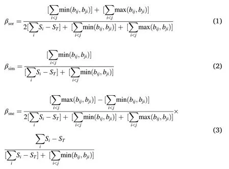
where Siis the total number of species in cell i,STis the total number of species in a given LGA,bij,bjiare the number of species exclusive to cells i and j, respectively. Compared with the formula of pairwise Sørensen dissimilarity,i.e. (b +c)/(2a+ b + c), where a is the number of shared species between two cells,b is the number of species unique to the poorest site and c is the number of species unique to the richest site (Baselga,2010),can be regarded as the multi-site analogue of a;as the multi-site analogue of b andas the multi-site analogue of c(Baselga,2010).Based on a‘moving window’-like approach(Melo et al.,2009;Men′endez-Guerrero et al.,2020),we calculated βsorand decomposed it into βsneand βsimcomponents for all 1,487 LGAs using the R package‘betapart’(Baselga and Orme,2012).

2.6. Statistical analysis

To answer questions(i)and(ii),we first mapped βsorof all 1,487 LGAs together with species richness and visualised the distributions of βsneand βsimseparately. Then, we analysed the relationships between the three β-diversity metrics together with species richness (SR), weighted endemism (WE) and corrected weighted endemism (CWE) with elevation,longitude and latitude across the study area by Pearson correlation analyses. Next, all LGAs were assigned to different vegetation zones(Fig. A4.1 in Supplementary material Appendix 4) according to their geographical location to compare the differences of three beta diversity metrics between biogeographic zones.

To ensure the reliability of the multi-site beta diversity outcomes and to avoid the use of pseudo-replicates in the statistical analysis for addressing our question(iii),we selected 166 discrete, non-overlapping LGAs out of 1,487 LGAs based on two principles: (i) only LGAs with at least five cells(Qian et al.,2020)were selected;and(ii)maximizing the number of LGAs. For the subsequent spatial analysis, we excluded the three isolated LGAs of Hainan and Taiwan,and used the remaining 163 discrete LGAs(Fig.A4.2 in Supplementary material Appendix 4).

Multi-site β-diversity,i.e.the variation in species composition among cells of an LGA, is likely to be affected by environmental variation between these sites. In addition, differences in β-diversity between LGAs,might also be affected by general environmental differences between LGAs.The latter is linked to STof the multi-site β-diversity equations,i.e.,the species richness of LGAs and the fact that species richness is often controlled by climate variables like mean annual temperature (Kraft et al., 2011). Thus, for exploring the relative impact of current climate and past climate change on βsorand its true turnover and nestedness components,we calculated both the mean and standard deviation terms(potentially meaningful explanatory variable for measuring variability in species composition among cells) of eight climate predictors (Table 1)within each of the 163 selected LGAs.

As current (1970–2000) climate predictors, we used mean annual temperature, annual precipitation, temperature seasonality and precipitation seasonality (available from WorldClim v2.0, Fig. A4.3 in Supplementary material Appendix 4). Our predictors of past climate change reflect how similar the current climate of each pixel is relative to LGM(averaged over the three GCMs of the LGM period), with higher values indicating greater fluctuation and comprised temperature anomaly,precipitation anomaly, temperature-change velocity (TCV) and precipitation-change velocity (PCV) (Fig. A4.4 in Supplementary material Appendix 4).TCV and PCV are distance-based velocities proposed by Hamann et al. (2015), that is, first calculating the minimum distance from a grid cell with current climate to a grid cell with similar LGM climate, and then dividing this distance by the year difference between the two time periods. We used ±0.25°C and ±25 mm as thresholds of similarity for temperature and precipitation, respectively. The importance of the above climate-related drivers in explaining species diversity has been demonstrated previously, especially at large scales (Sandel et al.,2011;Calatayud et al.,2016;Shrestha et al.,2018;Alahuhta et al.,2020).

To avoid co-linearity,we excluded the MAPmeanfrom the multivariate analysis because it was strongly correlated with the MATmean(r > 0.7 listed in Table A4.3 in Supplementary material Appendix 4, Dormann et al.,2013).VIF values for all used predictors are less than 5(Table 1).Strong spatial autocorrelation was detected in the residuals of the OLS multi-predictor regression models built for each β metric through Moran's I test,which could result in biased parameter estimates and incorrect error probabilities (Kühn et al., 2009). We thus used simultaneous autoregressive (SAR) model (spatial error, SARerr) following Dormann et al. (2007). First, we tested two key parameters in SARerrmodels for each β metric against all 15 predictors,that is neighbor distance(a series of distances in steps of 150 km from 150 to 6,000 km)and spatial weights(row-standardized, binary and variance-stabilizing coding schemes),based on minimizing the sum of the absolute Moran's I values for the first 20 distance classes(i.e.minRSA,see Kissling and Carl,2008).Second,we reduced the number of predictors by searching for models with the highest Pseudo-R2within two units of delta AIC of the minimum AIC model(Burnham and Anderson,2002).All analyses were performed in R version 4.0.2 (R-Core-Team, 2020), SARerrmodels were implemented using the ‘spdep’ package (Bivand et al., 2013). The complete analysis workflow is illustrated in Fig.1.

3. Results

3.1. ESM performance and relative importance of predictors

A Wilcoxon signed-rank test showed that AUC and TSS scores of the four algorithms ranked as follows: CTA > ANN > GLM ≈MAXENT(Fig.2a and b).Overall,the mean AUC and TSS scores of all ESMs were 0.991±0.015 and 0.950±0.068,respectively,indicating that our ESMs had an excellent prediction ability (Table A4.4 in Supplementary material Appendix 4).The relative importance of the seven sets of predictorsin shaping the distributions of Lauraceae species differed markedly;temperature seasonality was the most important, followed by precipitation of the warmest quarter, mean diurnal range and temperature anomalies(Table A4.1 and Fig.2c).

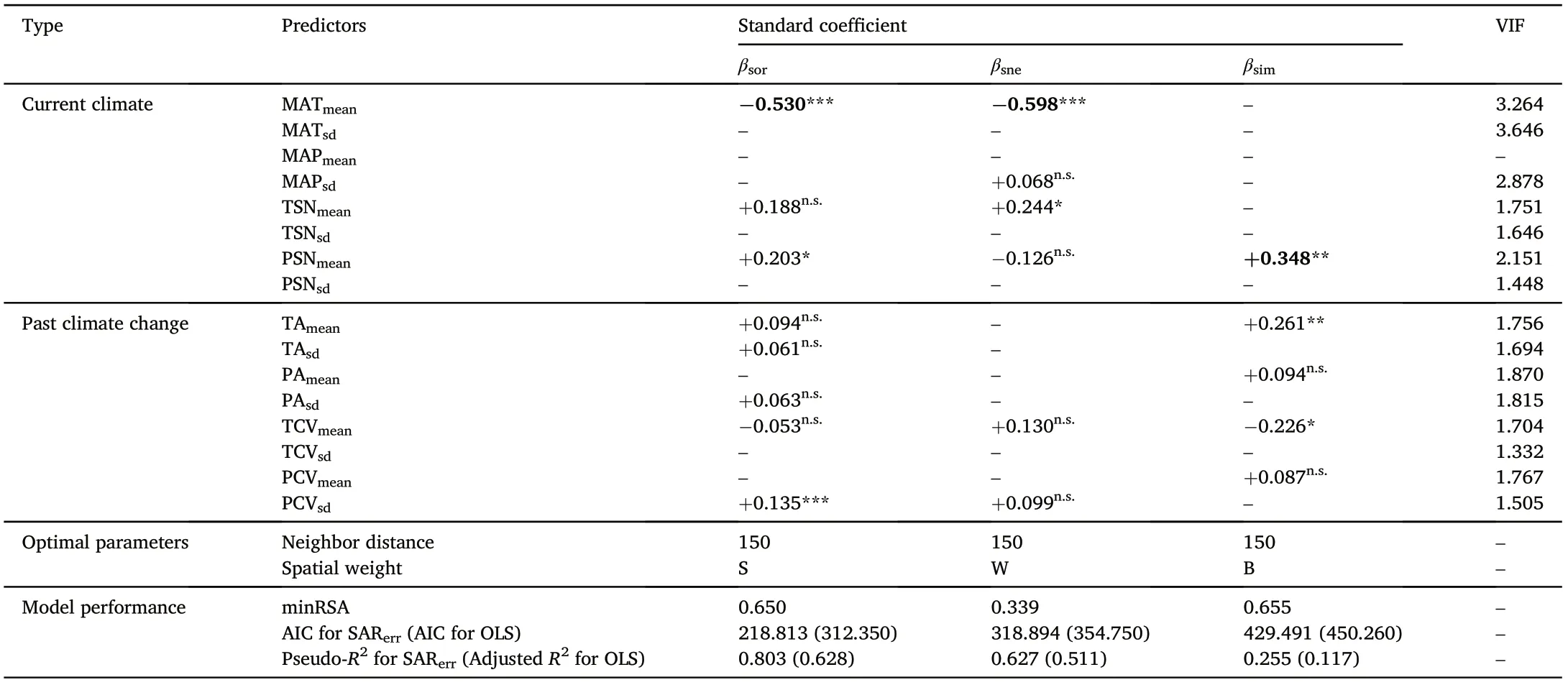
Table 1 Best fitted SARerr models predicting Sørensen-based multi-site dissimilarity(βsor)and its underlying true turnover(βsim)and nestedness(βsne)components for Chinese Lauraceae.

3.2. Alpha and beta diversity patterns of Lauraceae species

Species richness (SR), weighted endemism (WE) and corrected weighted endemism(CWE)of Lauraceae showed a clear negative correlation along the latitudinal gradient (R ＝-0.8, -0.75 and -0.38,respectively,in Fig.3a),with the highest quantile values(SR ∊[81,153])in the southernmost mainland of China(Fig.4a).In contrast,β-diversity(βsor)exhibited a clear positively correlated latitudinal gradient(R ＝0.57,Fig. 3b), with the highest quantile values (βsor∊[0.52, 1.00]) at the boundaries of deciduous and evergreen broadleaf forest zones,as well as in the Qinghai-Tibet Plateau,forming a horizontal bandingpattern around 30°N crossing central China(Fig.4a;Fig.A4.6 in Supplementary material Appendix 4).The distribution of the nestedness component(βsne)showed a clearer positively latitudinal gradient(R ＝0.63,Figs.3b and 4d)than that observed for βsor, but the true turnover component (βsim) did the opposite(R ＝-0.15,Figs.3b and 4c).In addition,the correlations of the above diversity indices are less pronounced for longitudinal and altitudinal gradients than for the latitudinal gradient(Fig.3b).We found that most of the places with high βsorvalues also revealed high βsnevalues((FFiiggs.. 44aa,,dd aanndd 55)).Notably,we identified 19grids characterized not onlyby a high species richness(107±5)but also by a high βsorvalue(0.392±0.019)and a large number of species endemic to China(62±5)(Fig.4b;Table A4.5 in Supplementary material Appendix 4).

3.3. Drivers of beta diversity

Our best fitted SARerrmodels significantly improved the model performance (AIC and Pseudo-R2) and reduced the autocorrelation of residuals(minRSA,see Fig.A4.5 in Supplementary material Appendix 4)compared to multivariate OLS regressions (Table 1). Overall, the multisite βsorand its βsneand βsimof Lauraceae in China were better explained by current rather than historical climate, and the effects of climate mean terms were stronger than the standard deviation terms.Among all the current and historical predictors, the spatially correlated MATmeanis the strongest predictor of the βsor(-0.530)and plays also an important role for the βsne(-0.598)component(Table 1). PSNmeanwas detected as the strongest predictor of βsim(+0.348),followed by TAmean(+0.261).

4. Discussion

The present study indicates opposing spatial patterns of α- and β-diversity in Lauraceae,with β-diversity gradually increasing from southern to central China. The underlying components of β-diversity, i.e. true turnover and nestedness, were mainly driven by different current climatic factors, including mean annual temperature and precipitation seasonality.

4.1. General patterns of α- and β-diversity in Lauraceae

Our results demonstrate a strong negative correlation between α-diversity(SR, WE and CWE)and latitude for Lauraceae. This is consistent with the latitudinal gradient of woody species α-diversity of Chinese broadleaved evergreen forests (Xu et al., 2017) and the α-diversity of woody plants in China in general(Wang et al.,2012b),and also reflects the common trend of lower species richness at higher latitudes(Gaston,2000). In contrast, we found a clear positive correlation between β-diversity(βsor)and latitude.This positive latitudinal gradient,however,did not show up in the geographic distribution pattern of β-diversity of all woody plants in China(Wang et al.,2012a)and is also in contrast to the well-documented pattern of decreasing beta diversity from the equator to the poles(Qian and Ricklefs,2007;Kraft et al.,2011).These differences(α-diversity vs. β-diversity as well as this vs. other studies) might be explained by the differences originating from analyzing entire plant communities versus those considering a single plant family, as in our study. In fact, β-diversity studies have often reached different conclusions, and these differences can be attributed to the taxa studied, the spatial scale investigated, the statistical methods used, or the compiled data sources (Rahbek, 2005; Kraft et al., 2011; Soininen et al., 2018;Sreekar et al.,2018).

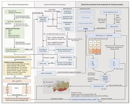
Fig. 1. Workflow of the present study.

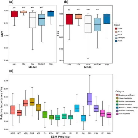
Fig. 2. Predictive abilities of the four independent algorithms and the final ESMs for all species, expressed as (a) the area under the curve of the receiver-operating curve(AUC)and(b)the true skill statistic(TSS).Symbols indicating statistical significance:ns,P>0.05;＊,P ≤0.05;＊＊,P ≤0.01;＊＊＊,P ≤0.001;＊＊＊＊,P ≤0.0001.(c) Boxplot (minimum, median, maximum, 25th and 75th percentiles) displaying the distribution of relative importance of each predictor to ESMs for all species.SRAD: solar radiation (kJ⋅m-2⋅day-1), NPP: net primary productivity (g C⋅m-2), MDR: mean diurnal range (mean of monthly (max temp – min temp)) (°C), PWQ:precipitation of warmest quarter (mm), WD: water deficit (mm), TH: topographic heterogeneity, EVIND: normalized dispersion of enhanced vegetation index, GPT:global pastures (%), GCL: global croplands (%), HII: human influence index, TA: temperature anomaly (°C), PA: precipitation anomaly (mm), TSN: temperature seasonality(standard deviation×100)(°C),PSN:precipitation seasonality(coefficient of variation:mean/SD×100)(%),CF:volumetric fraction of coarse fragments(%), BLD: bulk density (kg⋅m-3).

Furthermore,higher βsorvalues of Lauraceae species in mountainous regions (i.e. alpine zones) and at biogeographic boundaries (i.e. the boundaries between warm temperate and subtropical zones) is in line with the findings of Wang et al.(2012a),who showed that the β-diversity of Chinese woody plants is higher in the Qinghai-Tibet Plateau and the mountainous regions of central China than in other parts of the country.Similar results have been reported for other taxa and from other mountainous regions of the world, for instance, higher β-diversity of birds,mammals or amphibians detected in the Andes of South America, the Rocky Mountains in North America, the mountains of Central America(McKnight et al., 2007; Melo et al., 2009; McFadden et al., 2019), the Himalayas in Asia,or the Alps and the Balkans in Europe(Gaston et al.,2007).

4.2. Spatial distributions and proportion of the true turnover and nestedness components

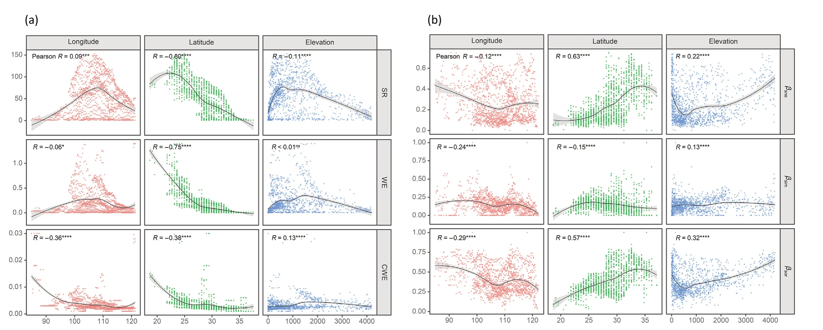
Fig.3. Elevational,latitudinal and longitudinal gradients of Lauraceae species richness(SR),weighted endemism(WE),and corrected weighted endemism(CWE)(a)and of βsor,βsim and βsne(b).The ftited lines in black denote the ‘loess smoothing curves (stat_smooth function of‘ggplot2 Rpackage) and the grey shaded areas denote the 95% confdience intervals. The independent statistical Pearson correlation coeffciient(R) is given.Symbols indicati’ng statistical signifciance: ns, P > 0.05; ＊, P ≤0.05’; ＊＊, P ≤0.01; ＊＊＊, P ≤0.001; ＊＊＊＊, P ≤0.0001.

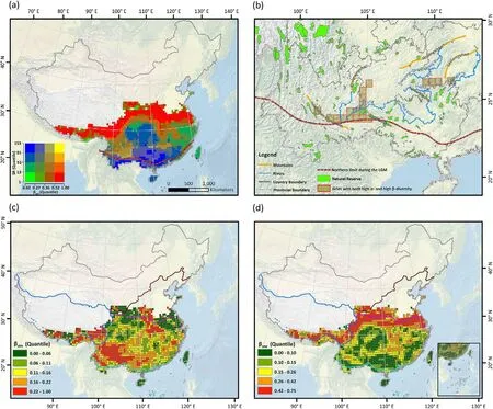
Fig.4. The species diversity patterns of Lauraceae in China simulated using an S-SDM framework.(a)Bivariate maps depicting both species richness(SR)and multisite Sørensen dissimilarity(βsor)patterns.Increases are depicted towards the red,blue and yellow ends of the spectrum.Each transition in colour shading translates to a 1/4 quantile shift in the value of the variables.(b)Grids with both high SR and βsor are recommended for biodiversity conservation of Lauraceae species.(c)The total dissimilarities explained by the true turnover(βsim)component.(d)The total dissimilarities explained by the nestedness(βsne)component.The projection system is the Asia North Albers Equal Area Conic,and the base map was obtained from Natural Earth(http://www.naturalearthdata.com/).The digitized northern boundary of the evergreen broadleaved forest biome during the Last Glacial Maximum is shown in (a) and (b), and the coloured lines in (c) and (d) represent the boundary of vegetation regions(see Fig.A4.1 in Supplementary material Appendix 4).(For interpretation of the references to colour in this figure legend,the reader is referred to the Web version of this article.)

When decomposing multi-site Sørensen dissimilarity (βsor) of Lauraceae into the true turnover (βsim) and nestedness components (βsne), a clearer positive latitudinal trend for the nestedness component(βsne)was found, but only a weak and negative correlation between true turnover(βsim) and latitude, which is supported by a global meta-analysis across multiple taxa(from bacteria to plants and mammals,see Soininen et al.,2018).On the other hand,Soininen et al.(2018)concluded that species turnover, consistently being the more prominent component of total β-diversity,while nestedness is more related to the latitude and intrinsic organismal features of the specific study area.This general conclusion is based on the meta-analysis of‘real’communities,i.e.composed of plants from multiple families (Soininen et al., 2018; Keil and Chase, 2019). In our study,however,the higher βsorin single Lauraceae family generated in the mountainous and biogeographic boundaries of center China was mainly due to a high nestedness component.The presumed cause might be that during the LGM, the evergreen forest underwent a strong contraction and retreated southwards to areas below 24°N (Ye et al.,2019b). After the Younger Dryas (～12.5 ka BP), broadleaf evergreen forests, including Lauraceae species, gradually expanded from tropical latitudes into the subtropical regions of East Asia and ended their expansion at 8,000–6,000 BP (Harrison et al., 2001). During long-distance northward migration from the past glacial refugia, environmental filtering and biological interactions lead to a gradual reduction in the number of species that successfully colonized, resulting in a gradual nestedness pattern (whereas the entire local species pool will have deciduous species of other families gradually replacing the evergreen species of Lauraceae, a competition process which was not considered in this study). Interestingly, the highest βsnewas detected at the boundary of the warm temperate deciduous and subtropical evergreen zones (Fig. 4d), rather than at the northern range limit of Lauraceae.Deciduous forests represent a legacy of the last glacial period and act as a barrier to the northward migration of evergreen taxa(Herzschuh,2020). In this process the differences in the migration capacity of deciduous (higher migration rates on average) and evergreen (lower migration rates)tree species affected the expansion distance from glacial refugia (Feurdean et al., 2013), resulting in clear distributional differences along the latitudinal gradient,with a more or less sharp transition between these two contrasting lifeforms. Since both lifeforms are represented in our study at the level of a single plant family,this might also contribute to the differences found between the continuous elevational and unimodal latitudinal βsnegradient. It may also partly explain the differences to other studies included entire plant communities.

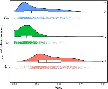
Fig. 5. Raincloud plot depicting distributions of multi-site Sørensen dissimilarity (βsor), its true turnover component (βsim) and its nestedness component(βsne).The“raindrops”represent the actual ratios,and the “rainclouds” and the boxplots summarize distributions of these ratios. A non-parametric Kruskal-Wallis test was performed to examine differences among the three β-diversity metrics. ＊＊＊ indicates significant differences (P < 0.001) in general.Different lower-case letters (a, b and c) indicate significant differences (P < 0.05) between two β-diversity metrics.

4.3. The relative effects of current climate and past climate change

The current mean annual temperature (MATmean) affected, in our analysis,the multi-site βsorand βsneof Lauraceae more than any historical climatic predictor. The gradual decrease in MATmeanfrom southern to northern China(Fig.A4.3 in Supplementary material Appendix 4)leads to a gradual decrease in the species richness of Lauraceae, reducing the number of shared species within each LGA of the detected boundary of warm temperate deciduous and subtropical evergreen zones (see Fig. A4.7 in Supplementary material Appendix 4) and thus increasing both βsorand βsne.Precipitation seasonality positively influenced the βsimof Lauraceae and was more substantial than past climate change.Xu et al.(2021)also suggested that climatic seasonality played a dominant role in the biodiversity of evergreen broad-leaved woody plants and is stronger than past climate variability. Seasonality is a unique feature of mid-latitude monsoon climates, influencing the distribution of most Lauraceae species (Fig. 2c) and the occurrence of mixed evergreen deciduous broad-leaved forests in China (Ge et al., 2019), as well as the richness of plant species in mountainous areas (Shrestha et al., 2018;Dakhil et al.,2021).

The standard deviation terms of both current and historical climate predictors were less important than the mean terms for explaining the three multi-site dissimilarity indices, but the direction of influence was always positive, suggesting that an increase in inter-cells climate heterogeneity increases the multi-site dissimilarity. In China, only high elevational regions were covered by glaciers during LGM period, and thus vegetation may have been less affected by past climate change(Qian et al., 2005) than in other parts of the world. In North America and Europe,where glaciation and ice shields were more pronounced,and the flora and fauna were more significantly influenced by ice ages(Qian and Ricklefs, 2007; Svenning and Skov, 2007; Saladin et al., 2020). For instance,climate history and dispersal ability explained well the turnover and nestedness components of β-diversity of amphibians in Americas(Dobrovolski et al.,2012).Nevertheless,even in such areas,which were generally more affected by LGM climate than our study area, a recent study showed that the strongest climate predictors of βsimof plant taxonomic and phylogenetic β-diversity across the Americas (tropical and temperate regions) were current mean temperature and temperature seasonality rather than climate change velocity since LGM (McFadden et al.,2019).

Climate stability and rapid climate change have different contributions and mechanisms to drive species true turnover and nestedness(Sandel et al., 2011; Dobrovolski et al., 2012; Ordonez and Svenning,2017;Blonder et al.,2018;Zwiener et al.,2018).Climate stability tends to result in smaller range sizes and endemism, which affects the true turnover component of β-diversity (e.g., Jansson, 2003), while rapid climate change filters for species with a high dispersal ability and large range size, which affects the nestedness component (e.g., Dobrovolski et al.,2012).The high species richness in the tropics,for example,may be due to increased endemism and smaller species ranges caused by climate stability (Jansson, 2003; Sheldon et al., 2011), which may result in higher βsimcompared with values in temperate regions.In our study,this was supported by the median values of βsimgrouped by biogeographic zones (Fig. A4.6 in Supplementary material Appendix 4) as well as validated by the negative relationship between βsimand TCVmean(Table 1).However,the increase in TAmeanreduced the number of shared species among an LGA(Fig.A4.7 in Supplementary material Appendix 4)and increased multi-site Simpson dissimilarity (βsim) in Lauraceae composition. Melo et al. (2009) suggested that the role of climate stability in influencing βsimmight reflect complex interactions with elevation and topography. This might also explain the positive correlation between TA and βsimin our study.For example,the tropical zone of China is heterogeneous and includes mountainous areas in the Yunnan plateau(high TA and high βsim,see Fig.4c;Fig.A4.4 in Supplementary material Appendix 4). Another interaction might occur between βsimand the species richness of LGA(Baselga,2010),which is affected by lower rates of species extinction and higher rates of speciation under stable climate conditions (Dynesius and Jansson, 2000). However, the low Pseudo-R2(0.255) of SARerrmodel for βsimmay produce some bias in the interpretation of the βsimcomponent and makes an accurate interpretation challenging.

4.4. Uncertainty and limitation

The ESM approach allows more taxa to be included, notably less frequent and rare taxa(e.g.,Scherrer et al.,2019;Tanaka et al.,2020),which is particularly important for our multi-site β-diversity assessment. The lack of inclusion of species with less than five occurrences might have biased the diversity assessment locally, but this study covered 78% of the Lauraceae species of our constructed list and focussed on large scale patterns. In addition, some models might not perform very well,but the impact of such“bad”models was reduced in our approach because the suitability maps are clipped by the convex hull of occurrences.

When calculating multi-site β-diversity, we used a 3 × 3 grid cell“moving window”approach,i.e.neighbouring cells were also focal cells of other local grid assemblages. For analysing the β-diversity of continuous grid data and at large spatial scales,this is a common approach(e.g.,Melo et al., 2009; McFadden et al., 2019; Men′endez-Guerrero et al.,2020). To ensure the reliability of the subsequent spatial statistical analysis, we used spatially non-overlapping LGAs. SARerrpredictors might be, however, somewhat over-interpreted since some of the variables were also used in the S-SDM framework. Fortunately, the mean annual temperature with the highest impact on β-diversity is unique.Finally, it must be mentioned that β-diversity related to species abundance is more meaningful in conservation biology(Baselga,2017;Chen et al.,2018),but in most cases,including our study,abundance data are not available at larger scales.

4.5. Implications for the conservation of Lauraceae

Conservation biologists are concerned about the overall global layout of protected areas and propose some general conservation strategies(Fuller et al., 2010; Watson et al., 2014). A hotspot analysis has shown that there are significant conservation gaps for broadleaved evergreen woody plants in China(Xu et al.,2017)and Lauraceae species richness is highly correlated with species richness in broadleaved evergreen forests(Song,2014),making it urgent to adapt the network of existing protected areas. When optimizing the location and size of protected areas, it is crucial to consider their complementarity,flexibility and irreplaceability(Gray et al.,2016),principles that fit well with the concept of β-diversity.In our study,we identified 19 grid cells(50 km×50 km)along with their neighbor cells as candidate areas for the prioritization of the conservation of Lauraceae. Specifically, we detected two areas located in the Liupan River Basin between the Ailao Mountains and the Wumeng Mountains,and in the Liujiang Basin between the Jiwan Mountains and the Wuling Mountains(Fig.4b).Such areas showing for Lauraceae at the same time a high β-diversity,high species richness,and a high number of endemic species can be mainly found within the subtropical zone of broadleaved evergreen forests (Table A4.5 in Supplementary material Appendix 4). Existing nature reserves (see Zhao et al., 2019), however,currently protect only a tiny part of these areas(Fig.4b).

5. Conclusions

Our large-scale study demonstrates a clear latitudinal pattern of β-diversity in Lauraceae, with different proportions of nestedness and true turnover depending on the biogeographic context.High β-diversity occurs in mountainous regions and at boundary of warm temperate deciduous and subtropical evergreen zones dominated by the nestedness component.Current climate explains β-diversity in Lauraceae better than climate anomalies or velocities since the Last Glacial Maximum. Especially,low values of current mean annual temperature are related to high β-diversity and its pronounced nestedness component, which should be further studied and better understood in times of global warming. Last but not least, and in contrast to analyses of β-diversity of entire species assemblages like of vascular plant,large-scale β-diversity studies of single plant families can provide complementary insights into the drivers of the diversity of evolutionarily more narrowly defined entities.

Ethics approval and consent to participate

Not applicable.

Funding

This work was financially supported by the National Key Research and Development Program of China (Grant No. 2016YFC0502101), the Second Tibetan Plateau Scientific Expedition and Research Program(STEP)(Grant No.SQ2019QZKK1603)and a Visiting Scholarship funded by the China Scholarship Council(Grant No.202004910612).

Authors’ contributions

ZL, YC and MPN conceived the idea, designed the simulation. ZL wrote the first draft; KP and LZ obtained the funding for the project;MAD, FZ and XT discussed and provided technical support; KL and XW collected and verified the species occurrences. BP and BW revised the manuscript. NEZ contributed to the finalization of this manuscript. All authors read and approved the final manuscript.

Consent for publication

Not applicable.

Declaration of competing interest

The authors declare that they have no competing interests.

Availability of data and materials

The Lauraceae species distribution maps predicted by the ensembles of small models as well as the data and code used for performing simultaneous autoregressive models are publicly available via the GitHub repository at https://github.com/optiforziyan/Lauraceae_beta_divesity.

Acknowledgements

The authors would like to thank Tianwen Tang and Meng Zhang for collecting the species observations, Xuefang Gong for her efforts in the phylogenetic diversity analysis initially conceived, Ruidong Wu for providing the shapefile of Chinese nature reserves,Kalle Ruokolainen for his constructive suggestion on variable selection and statistical analysis and Ingolf Kühn for checking the reliability of the spatial regression modeling.

Abbreviations

LGM Last Glacial Maximum

SR Species Richness

βsorSørensen dissimilarity

βsimSimpson dissimilarity (true turnover component of Sørensen dissimilarity)

βsneNestedness component of Sørensen dissimilarity

SRAD Solar Radiation

NPP Net Primary Productivity

MDR Mean Diurnal Range

PWQ Precipitation of Warmest Quarter

WD Water Deficit

TH Topographic Heterogeneity

EVINDNormalized dispersion of Enhanced Vegetation Index

GPT Global Pastures

GCL Global Croplands

HII Human Influence Index

TA Temperature Anomaly

PA Precipitation Anomaly

TSN Temperature Seasonality

PSN Precipitation Seasonality

CF Coarse Fragments

BLD Bulk Density

GLM Generalized Linear Model

CTA Classification Tree Analysis

ANN Artificial Neural Networks

MAXENT Maximum Entropy

SDMs Species Distribution Models

S-SDMs Stacked Species Distribution Models

ESMs Ensemble of Small Models

MaxSSS Maximizing the Sum of Sensitivity and Specificity

TSS True Skill Statistic

AUC Area Under the ROC Curve

LGA Local Grid Assemblage

SRLGASpecies Richness of the Local Grid Assemblage

MAT Mean Annual Temperature

MAP Mean Annual Precipitation

TCV Temperature Change Velocity

PCV Precipitation Change Velocity

Appendix A. Supplementary data

Supplementary data to this article can be found online at https://do i.org/10.1016/j.fecs.2022.100018.