A hybrid deep neural network based on multi-time window convolutional bidirectional LSTM for civil aircraft APU hazard identification

Di ZHOU, Xio ZHUANG, Hongfu ZUO

a Civil Aviation Key Laboratory of Aircraft Health Monitoring and Intelligent Maintenance, College of Civil Aviation,Nanjing University of Aeronautics and Astronautics, Nanjing 210016, China

b Department of Mechanical and Industrial Engineering, University of Toronto, Toronto M5S 3G8, Canada

c College of Science, Nanjing University of Aeronautics and Astronautics, Nanjing 210016, China

KEYWORDS Civil aviation;Convolutional neural networks;Deep neural networks;Hazard identification;Long short-term memory

Abstract Safety is one of the important topics in the field of civil aviation. Auxiliary Power Unit(APU)is one of important components in aircraft,which provides electrical power and compressed air for aircraft. The hazards in APU are prone to cause economic losses and even casualties. So,actively identifying the hazards in APU before an accident occurs is necessary. In this paper, a Hybrid Deep Neural Network (HDNN) based on multi-time window convolutional neural network-Bidirectional Long Short-Term Memory (CNN-BiLSTM) neural network is proposed for active hazard identification of APU in civil aircraft.In order to identify the risks caused by different types of failures, the proposed HDNN simultaneously integrates three CNN-BiLSTM basic models with different time window sizes in parallel by using a fully connected neural network.The CNN-BiLSTM basic model can automatically extract features representing the system state from the input data and learn the time information of irregular trends in the time series data.Nine benchmark models are compared with the proposed HDNN. The comparison results show that the proposed HDNN has the highest identification accuracy.The HDNN has the most stable identification performance for data with imbalanced samples.

1. Introduction

Continuous airworthiness risk management of civil aircraft is the research focus of airlines and aviation safety supervision agencies.The Federal Aviation Administration(FAA)indicates that the continuous airworthiness risk management process includes hazard identification, risk analysis, risk assessment and risk control. The hazard identification is the foundation of risk management.Only by accurately identifying the existing or potential hazards of the aircraft,the aircraft risk analysis and assessment can be carried out. Based on the risk analysis results, risk mitigation plan can be developed to reduce the safety accident.

Historically, the hazard identification was lagging and passive. Traditional hazard identification mostly begun after an accident or incident had occurred. At this time, the hazards of the aircraft had caused economic losses and even casualties.In recent years, airlines and aviation safety supervision agencies have been changing their focuses from traditional passive hazard identification to active data-driven hazard identification.Based on the active hazard identification, engineers can perform risk analysis and develop risk mitigation plans in advance to avoid aircraft damage and casualties.Moreover,the changes of flight schedule can be made in time to reduce the economic losses caused by flight delays.

Auxiliary Power Unit (APU) is a significant small power unit, which provides electrical power and compressed air for aircraft.The main functions of APU are as follows. Before the aircraft takes off, the APU provides electricity and compressed air to start the main engine. At the same time, APU provides electricity and compressed air (except Boeing787 series)to ensure the lighting and air conditioning in the cabin and cockpit so that the power of main engine can be totally used for ground acceleration and climbing. After aircraft landing,APU continues to supply lighting and air conditioning, which allows the main engine to shut down early to save fuel and reduce the noise of airport. Therefore, the status of the APU determines the operational performance and service quality of the aircraft.The hazard in APU will directly affect the normal use of ground cabin air conditioning, which will lead to flight delays in some airports with high turnover or limited ground support facilities. Apart from this, if the main engine suddenly stops during the flight at a high altitude (generally below 10000 m),the APU will provide the power for restarting the main engine.In this situation, if there exist hazards in APU, the main engine may fail to restart, which will lead to the occurrence of major accidents. Therefore, identifying the hazards of APU in advance is totally necessary so as to ensure flight safety and reduce flight delays.

Nowadays, many scholars have paid their attention on the operation of APU in aircraft by utilizing the data-driven deep learning method.Liu et al.proposed a hybrid Remaining Useful Life (RUL) prediction method by fusing an artificial intelligence-based model and a physics-based model to accurately predict the RUL of APU.Zhang et al. used a backpropagation feed-forward neural network to assess the starter degradation using the gas-path measurements of the APU.Liu et al. used an extreme learning machine optimized by a Restricted Boltzmann Machine(RBM)to predict APU performance parameters.Chen et al.developed a probabilistic prediction method based on Gaussian Process Regression (GPR)combined with Ensemble Empirical Mode Decomposition(EEMD) to evaluate the degradation of APU.Peng et al.used an adaptive feedback turning Sequential Importance Resampling (SIR) particle filter to diagnose the fault of APU.Yang et al.used Particle-based Filtering(PF)method to estimate the Time to Failure(TTF)of APU.Menon et al.used Hidden Markov Models (HMMs) for initial fault detection and diagnosis of APU.Although deep learning method has made a lot of achievements in the field of civil aircraft, as for the active APU hazard identification from the perspective of continuous airworthiness risk management,there have been fewer reports and literatures. So, in this paper, a multi-model framework named Hybrid Deep Neural Network (HDNN) is proposed to identify APU hazards from the risk management perspective.

Aircraft Communication Addressing and Reporting System(ACARS) is one of the effective ways to obtain aircraft safety monitoring data. The information of aircraft can be transmitted to the airline by the ACARS via wireless or satellite.ACARS reports are time series multivariate recorded over time, including spatial information and temporal information between variables. In this paper, the CNN-BiLSTM basic model that combines CNN and BiLSTM is proposed in HDNN to process the spatial information and temporal information in ACARS report. The adopted CNN-BiLSTM basic model exploits the good ability of CNN to remove the noise and extract valuable features from input data.The extracted valuable features are then input into the BiLSTM, which utilizes a unique structure of combining forward LSTM and backward LSTM to effectively catch sequence information.1The proposed CNN-BiLSTM basic model combines the advantage of two deep learning methods, thus improving the hazard identification performance of HDNN.

The time window size is an important parameter of the LSTM model.The LSTM model requires that the input data must have a specified time window size. Therefore, it is necessary to perform the time window preprocessing during the use of LSTM. In the deep learning model, the sliding time window method is often used for time window preprocessing of time series data. The sliding time window method converts the data into input variables for supervised learning. In this paper, the sliding time window method uses the data from the front time window as the input and the hazard label from the latter time as the output.Typically,the size of the time window is usually set as the smallest size of the data. This means that only one temporal dependency of the features is learned during the training of the model.Noteworthy, the different time window sizes have different influence on the identification accuracy of different hazards. FAA defines three types of failures for hazard identification,including early failures,random failures and wear failures.Each failure can cause different levels of hazard. When a small time window size is selected,the hazard precursors of wear failure cannot be adequately represented in the current time window. When large time window size is selected, the hazard precursors of random failures may be ignored as ordinary data fluctuations.In order to overcome these shortcomings,a multi-time window strategy is proposed in this paper. By utilizing the CNN-BiLSTM basic models with different time window sizes in HDNN, different time dependences can be learned.

The main insights and contributions of this paper are summarized as follows:

(1) A Hybrid Deep Neural Network (HDNN) is proposed to actively identify the hazards of APU from the perspective of risk management. The proposed HDNN can transform the traditional passive hazard identification after the accident into the active hazard identification before the accident.

(2) The combination CNN-BiLSTM model is adopted as basic model in the HDNN. The CNN in CNNBiLSTM is used to decompose multivariate time series data into univariate time series data to extract useful features from input data.The BiLSTM in CNN-BiLSTM is used to learn bidirectional long-term dependencies from the output of CNN. The adopted CNN-BiLSTM basic model exploits the advantages of two deep learning methods which can improve the hazard identification performance of HDNN.

(3) Three CNN-BiLSTM basic models with different time window sizes are utilized in the proposed HDNN. The multi-time window modeling strategy extends the time window size. The hyper-parameters of each basic model are set adaptively according to the time window size. In this way, the diversity of the basic model can be enhanced to be applicable to the hazard identification of multiple failure modes.

The outline of this paper is organized as follows. In Section 2, the active aircraft hazard identification framework of APU is carefully described. In Section 3, the methodology of the proposed HDNN is introduced. From Section 4 to Section 6, the experimental data, the parameter setting for each model, and evaluation indexes are introduced, respectively.In Section 7, the experimental results are analyzed in detail from various aspects. Finally, Section 8 provides the conclusion of our work.

2. Framework

The proposed active hazard identification framework based on HDNN for the APU of civil aircraft,with a schematic illustration shown in Fig. 1, can be described in a stage-wise fashion.The aircraft firstly transmits ACARS reports to the airlines via a ground-air network during the flight. Based on the accumulated ACARS reports, the normalized method is utilized to normalize the raw data. Then, according to the set time window size TWi, the normalized data is divided into different datasets by using the sliding time window method. After that,three CNN-BiLSTM basic models, which combine the advantages of CNN and BiLSTM, are employed in HDNN to process the normalized data with different time window sizes to obtain the initial identification results y. The details of CNN-BiLSTM working process are as follows. The CNN layer initially uses multiple filters to remove noise and extract valuable features from the input normalized data. The extracted valuable features are then input into the BiLSTM to catch temporal features. The caught temporal features are input to the fully connected layer and the softmax classifier to obtain initial hazard identification result. Finally, based on the initial identification results obtained by CNNBiLSTM basic models with different time window sizes, the fully connected neural network is utilized to combine the initial identification results to finally get the final identification results. The proposed HDNN can accurately identify the hazards of APU in aircraft. The identification results are further used for preliminary risk assessment to develop a risk mitigation plan. In order to avoid overfitting when training HDNN,two regularization methods including dropout (DP) and early stop are used.

3. HDNN

3.1. CNN

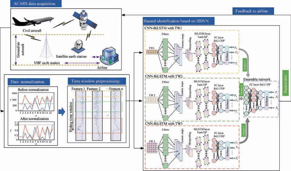
Fig. 1 Framework for active hazard identification of APU in civil aircraft.

CNN as a representative deep learning method, due to its excellent feature extraction and recognition performance, has been successfully utilized in image recognition and speech tasks. It has also attracted a lot of attention in the industrial field.CNN is a multilayer neural network. The weight sharing of CNN can make the neural network structure simpler and more adaptable.The structure of CNN is shown in Fig. 2. A typical convolutional network consists of convolution-pooling module and fully connected layer. The convolution-pooling module consisting of convolutional layer and pooling layer is used to extract features layer by layer.The structure of convolution-pooling module is shown in Fig. 3.

3.1.1. Convolutional layer

Convolutional layer is also called feature extraction layer,which is used to extract features and reduce the effects of noise.The primary function of the convolutional layer is to process the input features by using a series of convolution kernels and then output the processed feature map. Each convolution kernel in convolutional layer receives input from a group of kernels in a local region in the previous layer.The corresponding local regions are called local receptive fields. By introducing local receptive fields, convolution kernels can extract different types of features. The operation of convolutional layer is defined by

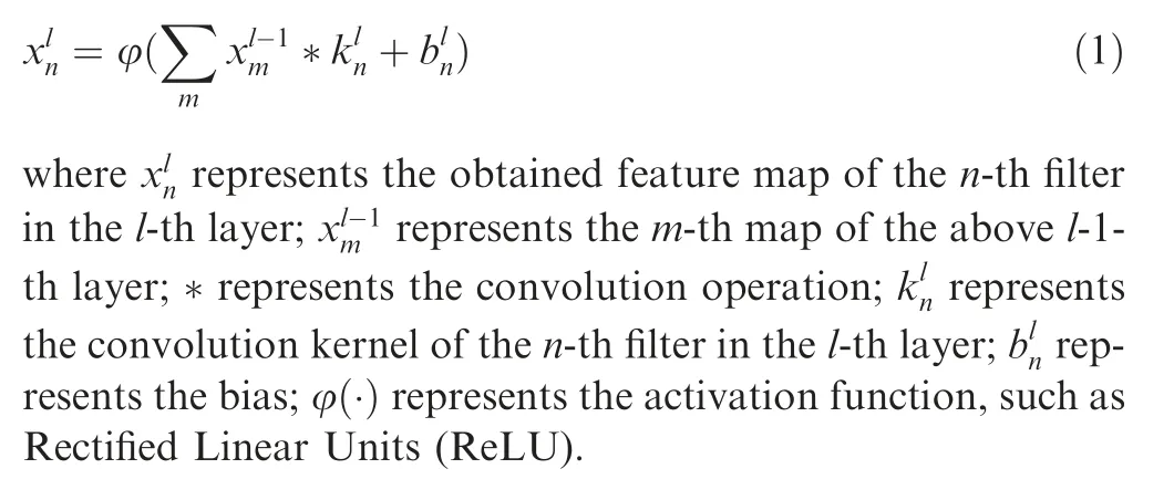
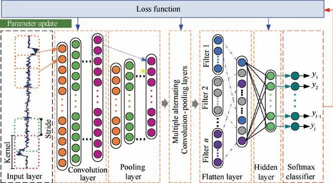
Fig. 2 Structure of CNN.

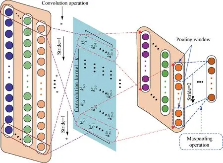
Fig. 3 Operation of convolution-pooling module.

3.1.2. Pooling layer

Pooling layer is also called sampling layer or feature mapping layer.It is mainly used to extract secondary features.The pooling operation is to down sample the convolutional feature map,thereby reducing the network size.Commonly used pooling method is maxpooling. It is defined by

3.1.3. Fully connected layer

The processed features of the last pooling layer are used as input to the fully connected layer. The primary function of the fully connected layer is to further extract features and connect the output to the softmax classifier. The fully connected layer is normally composed of many hidden layers. The operation of fully connected layer is described by

Then, a loss function is established by cross entropy function. Cross entropy function is an effective error metric function for pattern recognition that can be calculated by

where B is the number of sample; Trepresents the true value of the s-th sample;y represents the output of softmax classifier.

3.2. BilSTM

LSTM was first proposed by Hochreiter and Schmidhuber.In recent years, it was further improved and promoted by different works such as Refs.. LSTM overcomes the disappearance and explosion gradient of traditional RNN by introducing one memory state and multiple gating functions.These gating functions supply a memory-based architecture for determining the write and forget of information transferred to the memory state.In this paper, BiLSTM is used to learn the temporal features in the feature maps extracted by the convolutional layer.The BiLSTM consists of two independent LSTM layers that have the same input but transmit information in opposite directions. Compared with LSTM,BiLSTM can take full account of both historical and future information, thereby enhancing identification performance.The unit structure of LSTM and the network structure of BiLSTM are shown in Fig. 4.

The LSTM uses three gating functions to control the value of the added cell state c,which is used to save long term state.3The forget gating function fdetermines the amount of information retained from the last time cell state cto the present time cell state c. The input gating function icontrols the amount of information that the present input xsaves to the cell state c. The output gating function ocontrols the amount of information of the cell state cinput to the present output h. The LSTM has three inputs at time t, including the present time input value x,the last time output value hand the last time cell state c.The LSTM has two outputs at time t, which are the present time output value hand the present time cell state c. The output of LSTM at time t is updated from Eq. (5) to Eq. (10).

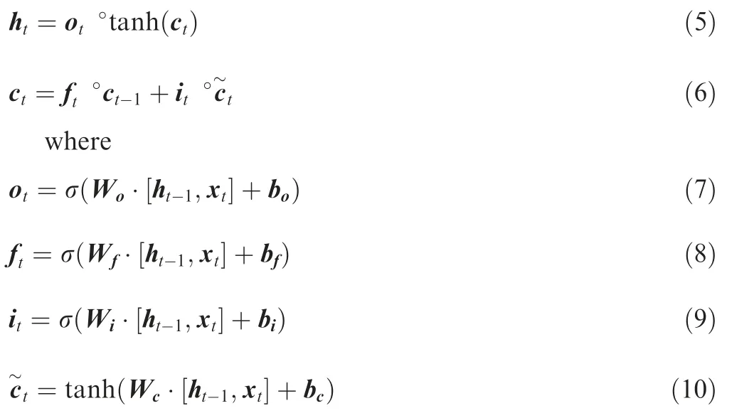
where σ（·） is the sigmoid function; Wand bare the weight matrix and bias of the forget gating function, respectively;Wand bare the weight matrix and bias of the input gating function, respectively; Wand bare the weight matrix and bias of the cell state, respectively; Wand bare the weight

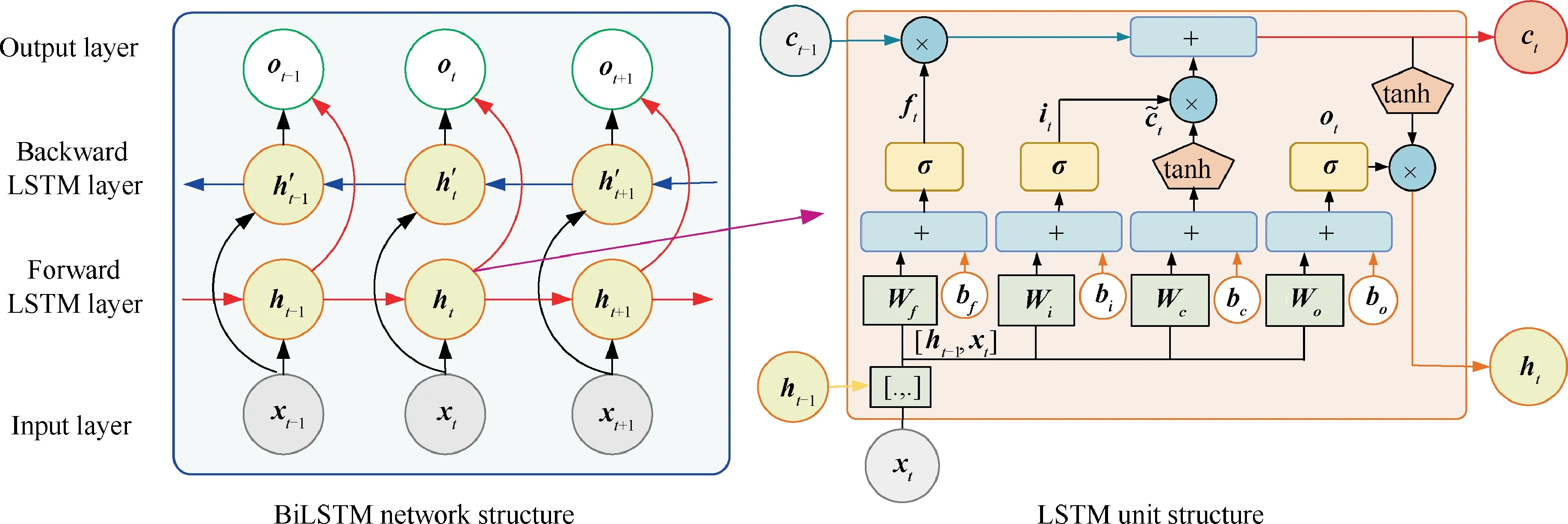
Fig. 4 Structure of LSTM and BiLSTM.

In the network structure of BiLSTM, the same input data are input to the forward LSTM layer and the backward LSTM layer to calculate the hidden state hof the forward LSTM layer and the hidden state hof the backward LSTM layer.The forward calculation is performed from time 1 to time t in the forward LSTM layer. The backward calculation is performed from time t to time 1 in the backward LSTM layer.The output of the forward hidden states and the backward hidden states at each time are obtained and saved.Then,the two hidden states are connected to calculate the output of BiLSTM.The calculation process of BiLSTM can be represented from Eq. (11) to Eq. (13).

where LSTM(●) represents the defined LSTM operation; Wand Wrepresent forward LSTM weight and backward LSTM weight, respectively; bis the bias of the output layer.

3.3. CNN-BiLSTM basic model

The CNN-BiLSTM is used as the basic model in the proposed HDNN.It can effectively extract the features of the input data.The CNN-BiLSTM basic model is composed of three parts.The first part is a CNN layer, which is used to extract important features from the input data.The second part is BiLSTM layer,which is used to learn the bidirectional long-term dependences from the output of CNN layer. The third part is two fully connected layers,which is used to map the learned feature representation to the label. The structure of CNN-BiLSTM basic model is shown in Fig. 5.

We suppose that there are P groups of different ACARS report in the input data. The monitoring time length of each group is N, where i ∈（1，P）. The sample number Nafter the sliding time window preprocess can be calculated by

where Sis time window size.

A zero-padding strategy is applied in the convolutional operation in order to maintain the feature dimension after convolution. The ReLU function is selected for nonlinear activation. The softmax classifier is used at the end of the network for classification. The input and output size of each layer in the basic model are shown in Table 1.In Table 1, Nrepresents the number of features;Nrepresents the number of filters; Srepresents the size of the pooling; Srepresents the number of neuron in the BiLSTM; Sand Srepresent the number of neurons in the first and second fully connected layers, respectively.

3.4. HDNN training process

The training process of the HDNN is divided into two stages,which requires two different training data including training data 1 and training data 2. The first stage is the training of basic models. The sliding time window method is used to preprocess the training data 1. When the time window size is 10,all feature values of the first 10 time points are selected as the first input to train the corresponding basic model. The hazard label at the 11th time point is selected as the supervised learning target value. Subsequently, step one unit along the timeline. The feature values of next 10 time points are selected as the second input with the hazard label of the 12th time point as the target value.After setting the hyper-parameters according to the size of the time window, the preprocessed training data 1 is input into the corresponding CNN-BiLSTM basic models to obtain the trained basic model. The training of the basic model is accomplished iteratively until all the training data 1 has been input into the model. The second stage is the training of fully connected ensemble network. The samesliding time window method is used to preprocess training data 2. The training data 2 with different Sis input into the trained CNN-BiLSTM to obtain the initial identification results. Then, the obtained initial identification results are input into the fully connected ensemble network for training.Finally, the trained HDNN is obtained. The training process of the HDNN is shown in Fig.6.In order to avoid overfitting when training HDNN, two regularization methods including dropout and early stop are used.

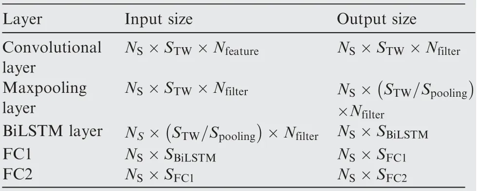
Table 1 Input and output size of each layer in basic model.

Fig. 5 Structure of CNN-BiLSTM basic model.

4. Experiment data

4.1. Data description

ACARS is one of the effective ways to obtain aircraft safety monitoring data. The ACARS collects and processes Quick Access Recorder (QAR) data from various aircraft systems in real time by using the Data Management Unit (DMU).The customized reports are compiled and generated in DMU. ACARS sends the customized reports in real time to the ground base station through the air-ground data link to achieve online monitoring of the aircraft. Unlike QAR data,which collects all monitoring data for an entire flight,ACARS is more flexible in its data collection.ACARS obtains the data of the parameter at a specific time point by setting the parameter value acquisition criteria.Targeted data collection can significantly reduce the amount of data used for analysis.

The A13 report is the MES/IDLE report of the APU which is generated by ACARS.The APU MES/IDLE reports are an average set of APU related parameters during the startup of each main engine and the APU idle state.The A13 report consists of four parts,including header,APU history information,APU operating parameters,and APU self-starting parameters.The format of the A13 report is shown in Fig.7.Symbols such as ‘‘XXXX”, ‘‘AAAA”, and ‘‘9999” in Fig. 7 will be replaced by real values during the flight. The header records the flight information of the aircraft, the flight phase for report generation and the parameters of the bleed valve. The history information of APU includes the APU serial number and the number of operating cycle hours. The values of APU operation parameters are recorded from N1 to S3 when the main engine of the aircraft is started. V1 records the values of APU self-starting parameters. The descriptions of A13 report parameters related to APU are shown in Table 2.

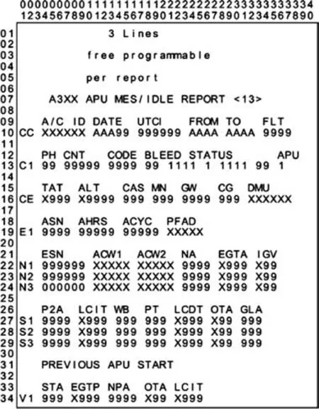
Fig. 7 Format of A13 report.

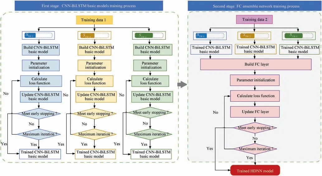
Fig. 6 HDNN training process.

2581 sets of A13 report data and the daily maintenance records from January 2015 to March 2017 are collected as sample data. In the reports, the control signals ACW1 and ACW2 are not able to indicate the state of the APU. In addition,some feature values are constant in the sample data,such as NA,WB,GLA,and IGV.These parameters should be manually removed from the report.Finally,the features reserved in the report are numbered 2, 3, 8, 10, 11, 12, 15, 17, 18, 19, and 20. The feature selection changes the feature dimension to 11.Some of these features are shown graphically in Fig. 8.

4.2. Hazard label setting

The airworthiness regulation part 25 issued by the FAA and its corresponding advisory circular AC 25.1309-1 indicate that it is necessary to evaluate the impact of a single system failure on the aircraft and crew.In addition,the FAA advisory circular AC 25.1309-1 classifies the failures of system into four classes according to their severity based on the direct or indirect effects on the aircraft and its occupants caused or contributed by one or more failures. In this paper, the system failure levels provided by the advisory circular AC 25.1309-1 are directly used to define the hazard labels of the APU system.A detailed description of each level is shown in Table 3..Different hazard labels are assigned depending on the level of failure. A higher hazard label results in more damage to theaircraft. Depending on the hazard label, different risk mitigation plans are developed by the airline or civil aviation organizations, such as issuing of emergency airworthiness directives,grounding or continuing flight.

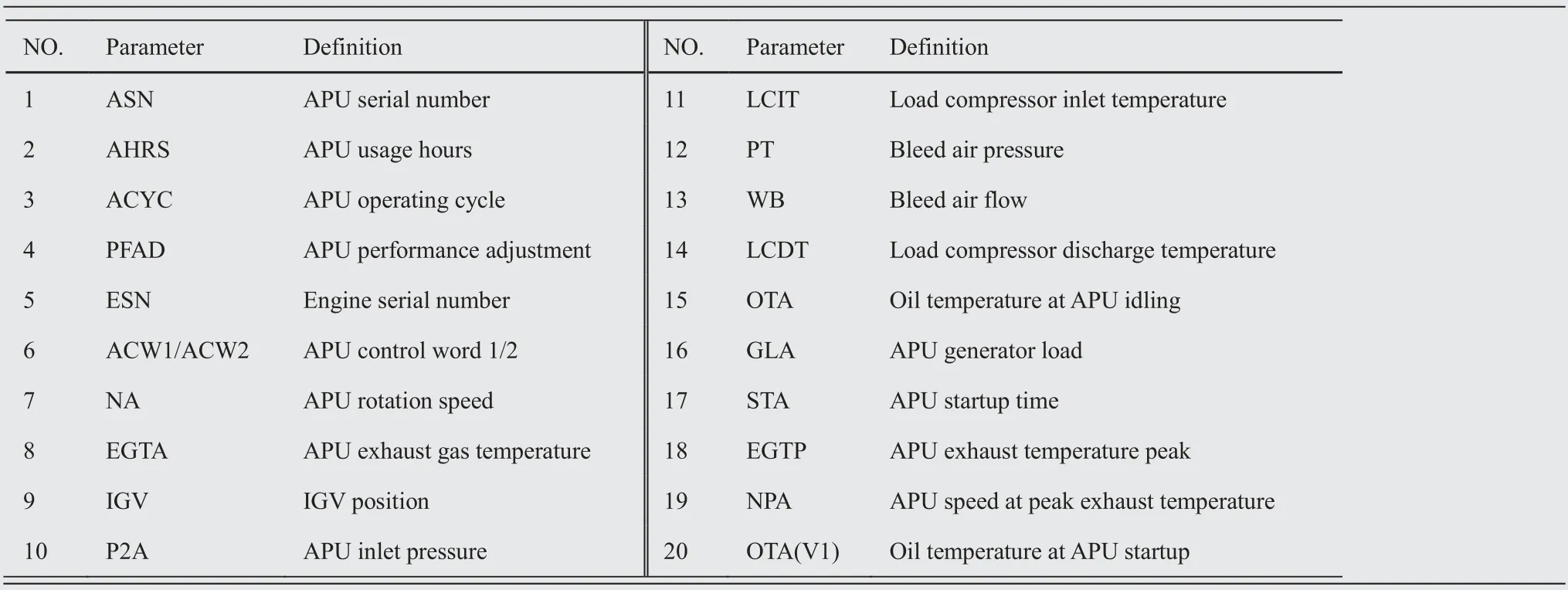
Table 2 Definitions of A13 report parameters related to APU.

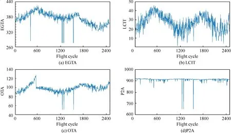
Fig. 8 Graphical visualization of report.

The Failure Mode and Effects Analysis(FMEA)document is completed as part of the aircraft system safety design and evaluation process. A summary of the failures, including failure modes, hazard levels, and cause codes, are recorded in the FMEA.Based on the FMEA and the collected APU maintenance records, the collected A13 report is marked with a hazard label.

Table 3 AC 25.1309-1 failure levels 34.

4.3. Data normalization

Normalizing the data to the same range can reduce the interference caused by the different value ranges of each parameter.All the data are normalized by Eq.(15)to be in the range[0,1]in this paper.

4.4. Dataset setting

In order to check the overall condition of aircraft,the‘‘Title 14 of the Code of Federal Regulations (14 CFR) part 91” issued by FAA states that all civil aircraft need be inspected at specific intervals and aviation maintenance technicians must conduct more detailed inspections at least once each 12 calendar months.Besides that, within 100 flight hours, an inspection of the aircraft must also be performed. In this paper, the time window sizes of the proposed HDNN are selected based on the FAA mandated inspection time. Since one A13 report is generated in one flight cycle, the data used in this paper use the flight cycle as the time unit.Conversion of flight cycles to flight hours is required to determine the time window size. According to the parameter values of DATA in the header of the collected report, the aircraft corresponding to the data used in this paper performs 1 flight mission per day. Therefore, 30 is selected as a time window size, which corresponds to the requirement of ‘‘each 12 calendar months” in the regulation.According to the parameter values of AHRS and ACYC in the collected report, the operating hours of the APU in one flight cycle are 5 to 10. Therefore, 10 and 20 are used as the other two time window sizes,which correspond to the requirement of‘‘within 100 flight hours”in the regulation.Therefore,the time window sizes are selected to be 10, 20, and 30 in the proposed HDNN. The training process of the proposed HDNN is divided into two stages,which requires two different training data including training data 1 and training data 2.The training data 1 accounts for 70% of the total data. The training data 2 accounts for 20%of the total data.The testing data accounted for 10% of the total data. In training data 2 and testing data,the data of the 10,20,and 30 data before the identified time point are combined as a set of input data. This means that each set of input data contains three sample data whose sizes are 10×11,20×11 and 30×11.The hazard label of the identified time point is used as the label of this set. The division results of the input data are shown in Table 4.

5. Parameter setting

5.1. Parameter setting for HDNN

The detailed parameter settings of HDNN are shown in Table 5. In this paper, multiple basic models with different time window sizes are integrated for hazard identification.The parameters of the basic model are set according to different time window sizes,so that the basic model has a completely different network structure. In the CNN-BiLSTM basic model,the number of convolutional filters,the number of neurons in the BiLSTM layer, and the number of neurons in thefirst fully connected layer in each basic model are all set as S. The number of neurons in the second fully connected layer is set as S/2.Such a setting contributes to the diversity of the basic model, so that different types of hazards can be better identified. The pooling layer size is set as 2×1. The stride of pooling layer is set as 2.The softmax classifier is used for classification. The Glorot uniform initializer is used to initialize the weights in the BiLSTM layer.The He uniform initializer is used in the other layers of the basic model.The batch size is set as 64 and the maximum training epoch is set as 100. The cross entropy function is selected as the loss function.The Adam optimizer is used with default parameters.The dropout and early stop are utilized to avoid overfitting. The default dropout rate is set as 0.5.

Table 4 Division results of input data.

Table 5 Parameter setting for HDNN.

The adopted fully connected ensemble network consists of three fully connected layers. The number of neurons in the three fully connected layers are set as 100, 50 and 20, respectively. ReLU is used as the activation function. The He uniform initializer is used to initialize the weights in all layers in the fully connected ensemble network. The softmax classifier is utilized at the end of the network for classification tasks.

5.2. Benchmark models

To illustrate the effectiveness of the proposed HDNN,two categories of benchmark models are used for comparison. In order to ensure that the parameters of the models used for comparison are consistent, a general setting principle based on the time window size is adopted.

5.2.1. Individual benchmark models

The individual benchmark models include DNN, CNN,BiLSTM and CNN-BiLSTM. In order to achieve the best identification effect, the time window sizes of DNN, CNN,BiLSTM and CNN-BiLSTM are set as 30.The main difference between each individual model is the neural network architecture of the first two layers. The first two layers of DNN individual benchmark model are two Feedforward Neural Network(FNN)layers.The first two layers of CNN individual benchmark model are two convolutional layers. The first two layers of BiLSTM individual benchmark model are two BiLSTM layers. The configurations of the last two fully connected layers of individual benchmark models are set to be consistent with the basic model with a time window size 30 in the proposed HDNN. The parameter setting of individual benchmark models are shown in Table 6.

5.2.2. Ensemble benchmark models

The ensemble benchmark models include Multiple Time Window (MTW) ensemble models and Single Time Window(STW) ensemble models. The MTW ensemble model replaces the basic model of HDNN with CNN and BiLSTM respectively.The STW ensemble models use a fixed time window size.The STW ensemble models are CNN ensemble model,BiLSTM ensemble model and CNN-BiLSTM ensemble model.The ensemble strategy is same in all ensemble benchmark models. The parameters of the basic models in each ensemble benchmark model are set as follows.

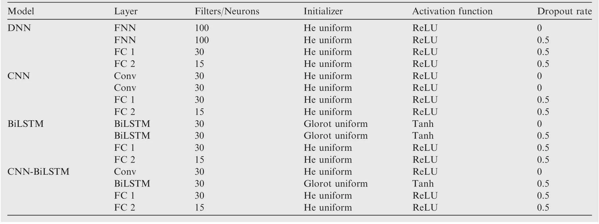
Table 6 Parameter setting for individual benchmark models.

(1) MTW CNN ensemble model

In the MTW CNN ensemble model,the CNN models with different time window sizes are used as the basic models to connect with the fully connected ensemble network. In the three CNN basic models, the time window sizes are selected as 10, 20 and 30 respectively. The number of filters in the two convolutional layers and the number of neurons in the first fully connected layer in the basic model are set as S. The number of neurons in the second fully connected layer is set as S/2.

(2) MTW BiLSTM ensemble model

The BiLSTM models with different time window sizes are used as the basic models to connect with the fully connected ensemble network.In the three BiLSTM basic models,the time window sizes are selected as 10, 20 and 30 respectively. The number of neurons in the two BiLSTM layers and the first fully connected layer in the basic model are set as S. The number of neurons in the second fully connected layer is set as S/2.

(3) STW ensemble model

The time window sizes of the basic models in the STW ensemble models are uniformly set as 30.In addition,for better model comparison, the network configuration of the basic models in the STW ensemble models are the same as that of the basic models in the corresponding MTW ensemble models.

6. Evaluation index

Four evaluation indexes are used for evaluating the performance of the identification model.First and foremost,we need to know that TP is the amount of positive labels identified as positive labels. TN is the amount of negative labels identified as negative labels. FP is the amount of negative labels identified as positive labels.FN is the amount of positive labels identified as negative labels.Precision is the ratio of the amount of samples correctly identified as positives to the amount of samples identified as positives.Recall is the ratio of the amount of samples correctly identified as positives to the total number of positives.L is the amount of label. l is the label. wis the ratio of samples in each label to the total sample.

6.1. Accuracy

6.2. F1 value

The F1 value is obtained by considering the balance between precision and recall, which makes it very suitable for imbalanced samples. The F1 value includes F1-score, Macro F1,Micro F1 and Weight F1.

(1) F1-score represents the identification performance of the different benchmark models for each label,which can be calculated by

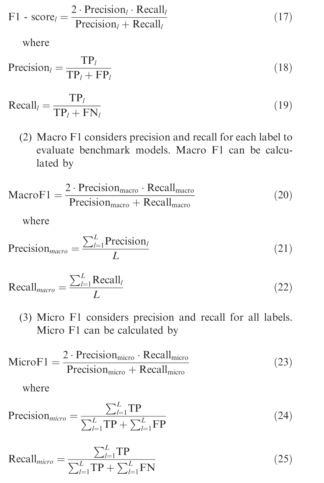
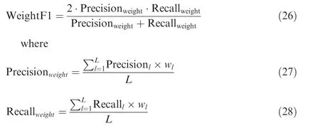
(4) Weight F1 is an improvement of Macro F1.Addressing the fact that Macro F1 does not consider the imbalance samples,Weight F1 considers the ratio of the number of samples in each label to the total number of samples.Weight F1 can be calculated by

7. Results and discussion

7.1. HDNN effect analysis

The testing data is input into the trained benchmark models and the trained HDNN for comparison. Each set of testing data contains three samples with different time window sizes.For individual models and STW ensemble models, samples with the time window size 30 in each set of testing data are used as input data. For the MTW ensemble models, samples with different time window sizes in each set of testing data are input into the corresponding basic models. Our work is performed based on a PC with Intel Core i7-9750H, 16 GB RAM and a NVIDIA GeForce RTX 2070 GPU. The confusion matrix and the Receiver Operating Characteristic(ROC) curve are used to qualitatively compare the identification performance of each model. The evaluation indexes are used to quantitatively compare each model. Each experiment is repeated ten times to reduce randomness. Fig. 9 shows the detailed identification accuracies of ten trials. The mean accuracy and standard deviation are calculated,as listed in Table 7.

The confusion matrixes of the benchmark models and the HDNN are shown in Fig. 10. The value in the confusion matrix is the sum of the ten trials. Each column of the confusion matrix represents the predicted label. Each row of the confusion matrix represents the true label. The values on the matrix diagonal represent the amount of correctly classified samples in each label in ten trials. The last column shows the percentage of correctly classified samples and incorrectly classified samples of all samples for each label. It can be concluded from the confusion matrixes that the number of correctly classified samples in the ensemble models is higher than that in the individual models. Compared with other ensemble models, the identification accuracy of each label of HDNN is higher than 81%, which shows the effectiveness and robustness of the proposed HDNN for the identification of different hazard levels.

The ROC curve plotted on a two-dimensional plane is commonly utilized for evaluating the identification performance of a model.The closer the ROC curve is to the upper left corner,the higher the identification accuracy is.The identification performance can also be compared by calculating the area under the ROC curve(AUC)of each label.The closer the AUC is to 1, the better the identification performance of the model for that label is. In addition, to further compare the identification performance of each model, the multi-classification AUCis calculated by

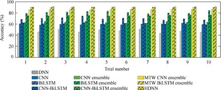
Fig. 9 Accuracies of ten trials.

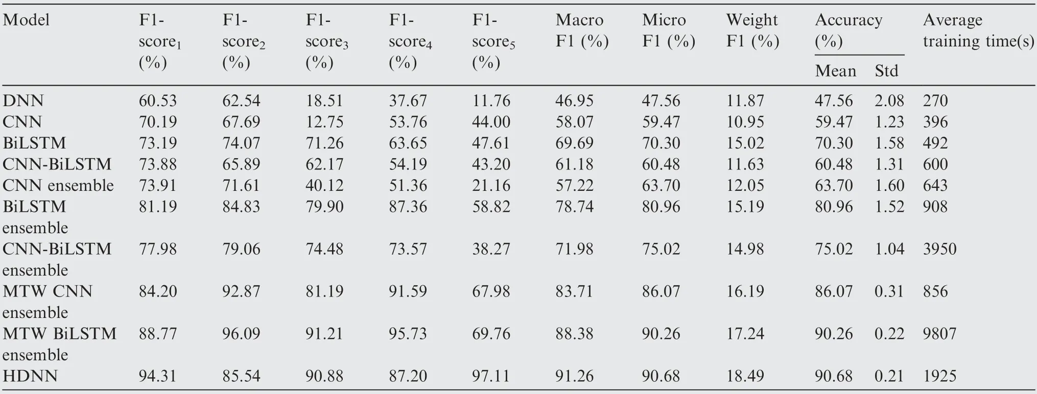
Table 7 Evaluation indexes for different models.

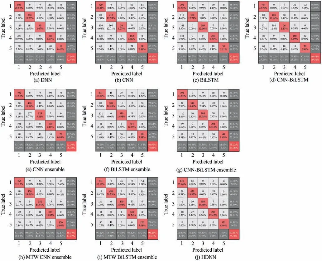
Fig. 10 Confusion matrixes of different models.

The ROC curves for each label of different models and their corresponding AUCs are show in Fig. 10 and Fig. 11. In Fig. 11, the green line represents the ROC curve with catastrophic hazard level. The blue line represents the ROC curve with severe major hazard level. The yellow line represents the ROC curve with major hazard level.The purple line represents the ROC curve with minor hazard level.The red line represents the ROC curve with no influence.

Fig.11 shows that the ROC curves of the ensemble models are closer to the upper left corner than the ROC curves of the individual models. Among the STW ensemble models, the ROC curves for all labels of the BiLSTM ensemble model are the closest to the upper left corner. The ROC curves of the MTW ensemble models are better than those of other models.As can be seen from Fig.12,the AUC of CNN-BiLSTM is slightly larger than that of the other three individual models.The AUC of the STW ensemble model is superior to that of the individual model. But the improvement is not obvious.The AUC of the MTW ensemble model is higher than that of the other benchmark models. From Fig. 11 and Fig. 12, it can be concluded that the ROC curves and AUCs of the MTW ensemble models are very close to each other. Moreover, the ROC curves for all labels of the MTW ensemble models are close to the upper left corner. The AUCis used to further compare the identification performance of the MTW ensemble model. The AUCof MTW CNN ensemble model is 0.972.The AUCof MTW BiLSTM ensemble model is 0.980. The AUCof HDNN is 0.984, which is higher than the other MTW ensemble models.

Through the confusion matrix, the precision and recall of each corresponding label can be calculated. The calculation results of precision and recall are shown in Table 8.According to Table 8,the F1 value can be calculated as shown in Table 7.The F1-score is used to illustrate the identification performance of the benchmark model for each hazard label. The F1-score is shown in Fig. 13. The F1-score values of the MTW ensemble models are higher than those of other benchmark models. Moreover, the MTW ensemble models show more stable identification performance in various hazards.However, due to the imbalance of samples, MTW CNN ensemble model and MTW BiLSTM ensemble model have poor identification performance for the hazard of catastrophe.The HDNN has a stable identification performance for all the hazard labels, which is unaffected by the imbalanced samples.

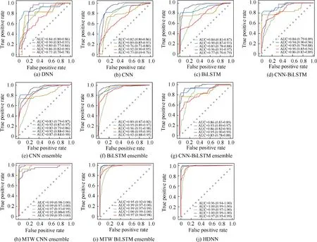
Fig. 11 ROC curves of different models.

Fig. 12 AUC of each label in different models.

Other F1 values are used to compare the identification performance of the model from a comprehensive perspective,which are shown in Fig. 14. The F1 values of BiLSTM are the highest among the four individual models. Among theSTW ensemble models, the F1 values of the CNN ensemble model are the lowest. The F1 values of the MTW ensemble models are superior to those of other benchmark models.Among the F1 values,the calculation of Macro F1 and Micro F1 does not consider the imbalance of the samples.The Macro F1 values of MTW ensemble models are 83.69%,87.88% and 90.98%,respectively.The Macro F1 value of HDNN improves by 8.71% and 3.53% than that of other two MTW ensemble models, respectively. The Micro F1 values of MTW ensemble models are 85.59%, 90.25% and 90.68%, respectively. The Micro F1 of HDNN improves by 5.95%and 0.47%than that of other two MTW ensemble models, respectively. The differences between Macro F1 and Micro F1 of the MTW ensemble models are not obvious. The Weight F1 is an improvement of Macro F1.The calculation of Weight F1 considers the ratio of the number of samples in each label to the total number of samples. The Weight F1 of MTW ensemble models are 16.20%, 17.08% and 18.43%, respectively. The Weight F1 of HDNN improves by 13.77% and 7.90% than that of other two MTW ensemble models,respectively.The HDNN has better identification performance for imbalanced samples than the other two MTW models.

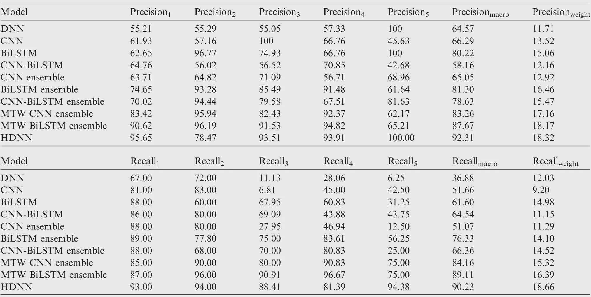
Table 8 Precision and recall for different models (%).

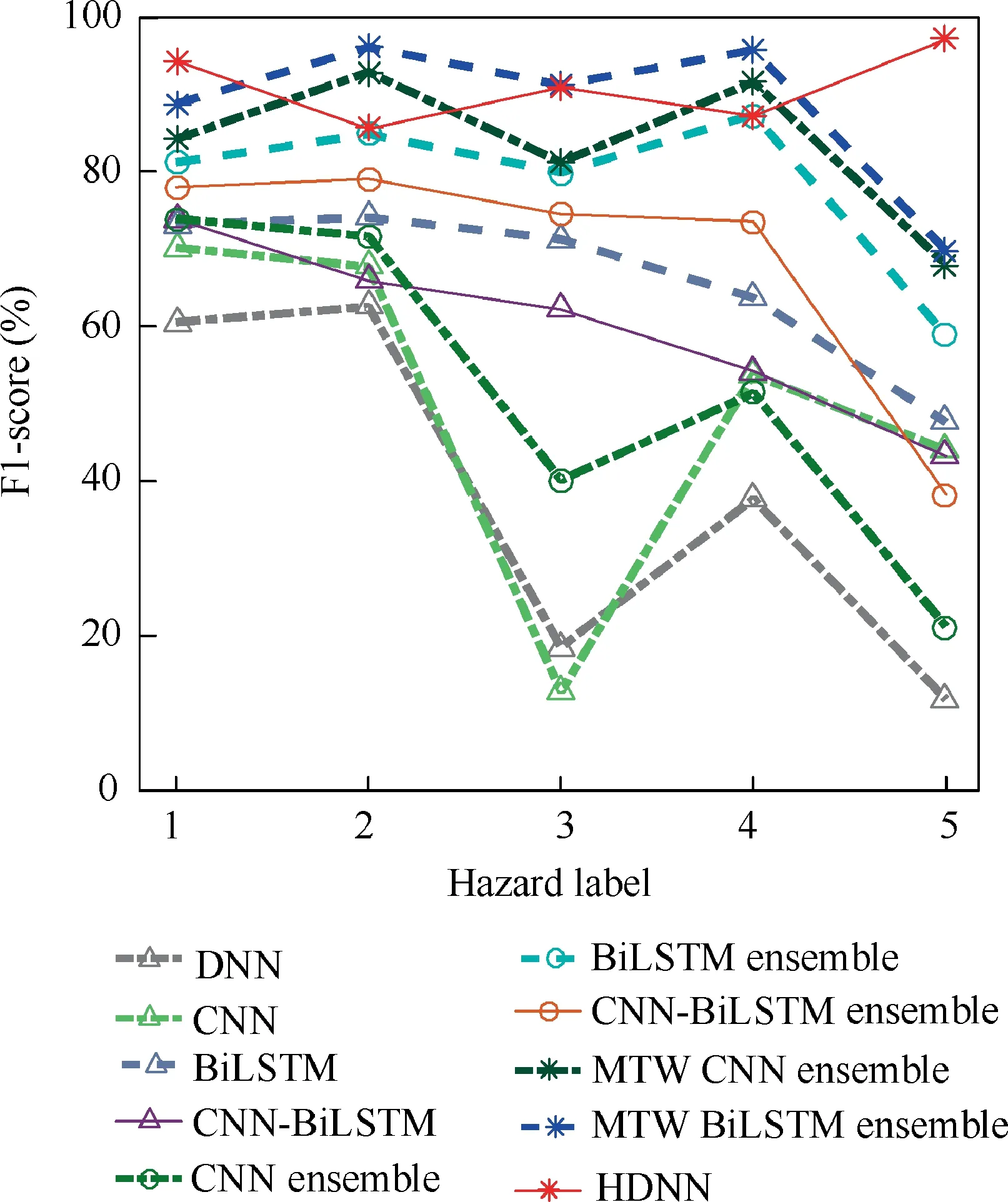
Fig. 13 F1-score of different models.

In the terms of accuracy, compared with the DNN model,the accuracy values of CNN,BiLSTM and CNN-BiLSTM are significantly improved. Among these three models, BiLSTM has the highest identification accuracy.The CNN has relatively poor identification performance. The identification performance of three STW ensemble models is a little better than that of their corresponding individual models. The identification performance of MTW ensemble models is significantly superior to that of other models.

In the MTW ensemble models, the identification accuracy of HDNN is 90.68%. The identification accuracy of MTW BiLSTM ensemble model is 90.25%. Compared with MTW BiLSTM ensemble model, the identification accuracy of HDNN has only improved by 0.43%.However,from the computational time cost,it can be seen from Fig.14 that the MTW BiLSTM ensemble model takes much longer for training than other models.It is due to the fact that the amount of information,which BiLSTM needs to deal with,grows rapidly with the size of the time window. Compared with MTW BiLSTM ensemble model, the proposed HDNN is able to save large amount of calculation cost while keeping nearly the same accuracy.

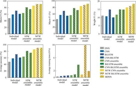
Fig. 14 Evaluation indexes of different models.

To further illustrate the superiority of the proposed HDNN,the HDNN is compared with the CNN-BiLSTM individual model and the STW CNN-BiLSTM ensemble model.The identification accuracy of HDNN is 29.66% higher than that of CNN-BiLSTM individual model and 15.26% higher than that of the STW CNN-BiLSTM ensemble model.The significantly improved identification performance of the HDNN mainly comes from two factors.One factor is that the HDNN has multiple basic models with different time window sizes while the STW ensemble model has a fixed time window size.This multi-time window modeling strategy expands the size of the time window of the basic model.The other factor is that the HDNN utilizes the fully connected neural network to ensemble the basic models. This ensemble strategy further improves the identification accuracy.

7.2. Multi-time window strategy effect analysis

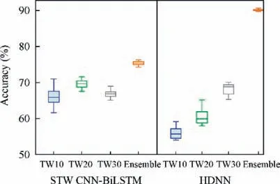
Fig. 15 Identification accuracy values of STW CNNBiLSTM ensemble model, HDNN and their corresponding basic models.

In the HDNN, the number of filters in the CNN layer, the number of neurons in the BiLSTM layer and the number of neurons in the two fully connected layers of three basic models are set according to the time window sizes.In the STW CNNBiLSTM ensemble model, the time window sizes of all the basic models are set as 30. However, the number of filters in CNN layer, the number of neurons in BiLSTM layer and the number of neurons in two fully connected layers of the three basic models are the same as the basic models in HDNN.The identification accuracy values of the STW CNNBiLSTM ensemble model, HDNN and their corresponding basic models are shown in Fig. 15. It can be seen from Fig. 15 that the identification accuracy values of three basic models in the STW CNN-BiLSTM ensemble model are almost the same. With a fixed time window size, the identification accuracy of the basic model of the STW CNN-BiLSTM ensemble model shows a downward trend with the increase of neurons. Different from the STW CNN-BiLSTM ensemble model,the identification accuracy values of three basic models in the HDNN with multi-time window sizes increase rapidly with the increase of the number of neurons. This shows that simply adding more neurons does not significantly enhance the learning capacity of the basic model. Instead, it will increase the tendency of overfitting. The adopted multi-time window modeling strategy can effectively improve the identification performance of the model and avoid overfitting.

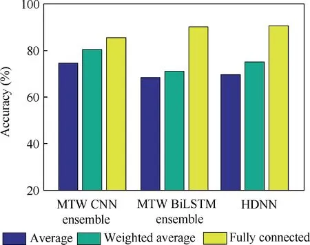
Fig. 16 Comparison of ensemble strategy.

7.3. Ensemble strategy effect analysis

In order to verify the effect of the fully connected neural network based ensemble strategy,two average ensemble strategies are used for comparison. One is the simple average ensemble strategy,which integrates the identification result of each basic model with the same weight.The other is the weighted average ensemble strategy, which assigns weight to each basic model based on the time window size.The identification accuracy values of MTW ensemble models with different ensemble strategies are shown in Fig. 16. It can be concluded that compared with the simple average ensemble strategy, the weighted average ensemble strategy slightly improves the identification accuracy. Compared with the two average ensemble strategies, the fully connected neural network based ensemble strategy adopted in this paper significantly improves the accuracy of hazard identification.

8. Conclusions

In this paper, a HDNN is proposed to actively identify the hazard of APU for civil aircraft based on ACARS reports.Considering the temporal data characteristics of different failure models, the proposed HDNN utilizes multiple CNNBiLSTM basic models with different time window sizes to obtain initial identification results. The initial identification results of the basic models are integrated by a fully connected neural network to obtain the final hazard identification results.After that,based on the accumulated ACARS report,the identification performance of the HDNN is verified by comparison with various benchmark models.The comparison result shows that the proposed HDNN has the best identification accuracy and F1 values.Additionally,the HDNN also has good identification performance for data with imbalanced samples. Further analysis results show that the multi-time window modeling strategy and fully connected neural network based ensemble strategy adopted in the proposed HDNN can significantly improve the accuracy of hazard identification.

The authors declare that they have no known competing financial interests or personal relationships that could have appeared to influence the work reported in this paper.

s

This study was co-supported by National Natural Science Foundation of China(No.U1933202),Natural Science Foundation of Civil Aviation University of China (No.U1733201),China Scholarship Council (CSC) (No. 201906830043) and Postgraduate Research & Practice Innovation Program of Jiangsu Province, China (Nos. KYCX18_0310 and KYCX18_0265).