Higher Accuracy Shape-preserving Modeling Based on the Two-level Fitting Method

Yang DangfuLiu Shengjun,2Liu PingboLiu Xinru,

(1.School of Mathematics and Statistics,Central South University,Changsha410083,China;2.State Key Laboratory of High Performance Complex Manufacturing,Central South University,Changsha410083,China;3.College of Computer and Information Engineering,Central South University of Forestry and Technology,Changsha410004,China)

Abstract Compactly supported radial basis function(CSRBF)has been widely used in surface modeling methods to interpolate or approximate the given data,which avoids solving a large dense linear system with a proper supported radius.The surfaces reconstructed by the CSRBF-based method usually are not shape preserving,while the multivariate multiquadric quasi-interpolation results the lower approximation accuracy.In this paper,we introduce a two-level fitting method to conduct the shape-preserving modelling with a higher accuracy.An initial shape-preserving model is constructed by using the lower accuracy quasi-interpolation,and then a CSRBF-based networks interpolation is performed to compensate the errors between the initial fitting model and the given data,then the higher accuracy shape-preserving model can be obtained.Moreover,we discuss the choice of the smoothing factor in quasi-interpolation and the supported radius in CSRBF-based networks,and an empirical formula between them is constructed.The numerical examples demonstrate the performance of our method.

Key words Surface modeling Two-level fitting Multivariate multiquadric quasi-interpolation CSRBF-based networks Shape-preserving model

1 Introduction

The interpolation of functions from the given data is an important theme in many fields of science and engineering.However,we often have some additional requirements that we wish to confine to interpolation.For example,we know the quantity from which the data is sampled,is positive,monotonic or convex.Thus,it is important to construct a function which satisfies the underlying constraints.Many works have been done on the problem of shape preserving interpolation[1,2,3,4,5].They mainly used polynomial interpolation or spline interpolation with a certain continuity to solve it.

Among the interpolation methods,there is an important class of methods—radial basis function-based interpolation.Radial basis function(RBF)is a relatively simple multivariate function generated by a univariate function.Due to its simple form and good approximation behavior,more and more researchers construct interpolation functions with them,and have obtained better results during the last two decades[6,7,8,9,10,11,12,13].However,there has been little work done on the imposition of constraints for these interpolation methods by using radial basis functions.For RBF,in the special case of thin-plate splines for2D data,reference[14]showed how positivity can be imposed as a constraint.Reference[15]discussed several meshless methods for constrained scattered data interpolation and applied them on3D data.For the Shepard interpolation,reference[16]discussed the modified quadratic Shepard method,which interpolates scattered data of any dimensionality,can be constrained to preserve positivity.Recently,Wu[17]presented an algorithm to construct a kind of so-called shape preserving interpolating function with the use of compactly supported RBF(CSRBF)and a class of multiquadric quasi-interpolation(MQ-QI)operators.But,his method is only for curve construction.

In this paper,inspired from Wu’s idea[17],we will propose a method for shape preserving surface reconstruction from the given surface data.We first reconstruct an initial surface from the given points with a multivariate multiquadric(MMQ)quasi-interpolation operator,and then compensate the error between the initial surface and the given points with the CSRBF networks.In addition,to balance the efficiency and the accuracy,we provide a valid interval of the number of neighbors for RBF centers,and create a relationship between it and the smoothing factor in MMQ.

The remainder of this paper is organized as follows.In Section2,we introduce the basis of our method,CSRBF interpolation and MMQ quasi-interpolation(MMQ-QI).After that,in Section3,we construct a shape preserving interpolation function for surface reconstruction combining with a CSRBF networks interpolation operator and a MMQ-QI operator(abbr:MMQ-CSRBF),and discuss the determination of the shape parameters in detail.Then,in Section4,we give some numerical examples to compare the approximation capacity of our hybrid scheme with that of CSRBF networks interpolation method and MMQ-QI scheme.Following this,conclusions about this work and the future works are listed in the last section.

2 Preliminaries

2.1 Compactly supported radial basis function interpolation

Given a set of distinctive data{xi,fi}∈Rd×R,i=0,1,···,n,the radial basis function-based interpolant is a function

whereϕi(x)=ϕ(//x−xi//)is a basis function which depends on the Euclidean distance between any point x∈Rdand a given point xi∈Rd,the coefficients,λi,are determined by the following constraints

There are many choices for the basic functionϕwhich include the biharmonic splineϕ(r)=r,the triharmonic splineϕ(r)=r3,the thin-plate splineϕ(r)=r2log(r),the multiquadricϕ(r)=+c2,the Gaussianϕ(r)=exp(−c2r2),and the inverse multiquadricϕ(r)=(r2+c2)−1/2,wherecis the shape parameter.However,in order to ensure the uniqueness of the solution of the interpolation problem,the coefficient matrix generated by the basis functionϕin the linear system(2.2)should be positive definitely.In this paper,we take the compactly supported positive definite radial basis function[18]

whereρis the support size,andr=//p−q//is the Euclidean distance between a point p and a RBF center q.

The CSRBF methods(eg.CSRBF networks)can interpolate well on the given data set,but it is ineffective in shape preserving,as shown in Figs.1(b)and1(e).In Fig.1,the subfigure1(a)shows the original surface defined by a quadric polynomial

and the sampling pointsP(training points,also)on the surface.Fig.1(b)gives out the reconstructed surface with CSRBF networks interpolation directly from the pointsP.And the residual surface between the original surface and the reconstructed surface is shown in Fig.1(e).The maximum and the variance of the residuals are listed in Table1.Here,we randomly selectk=20in[4,35](h=1.2 by(3.8 ),correspondingly),and apply them for all examples in section4to show the robustness of the way to set the parameters in our proposed method.

2.2 Multivariate multiquadraic quasi-interpolation

Quasi-interpolation is a class of approximation methods for data fitting.Compared with the RBF-based interpolation,the quasi-interpolation method constructs the approximation formula directly with some approximating errors,but it can preserve the shape of given data well,as shown in Figs.1(c)and1(f).By using the linear combination of Hardy’s MQ basis

and low order polynomials to construct the kernel functionαi(x),Beaton and Powell[19]first proposed a univariate quasi-interpolation formula.However,the requirement of the derivative information of the approximating functionfat the endpoints prevents the practical use of this formula.Wu and Schaback[20]proposed an improved univariate quasi-interpolation formula without using the derivative values at the endpoints,and their formula is given by

where the quasi-interpolation kernelαi(x)is as follows

It has been proved that the MQ quasi-interpolation(2.6)preserves linear reproduction,monotonicity,convexity and variation-diminishing[20].

Ling[21]extended(2.6)to bivariate quasi-interpolation by using the dimension-splitting multi-quadric basis function approach.For a given data setP={xi,yj,fij}(i=0,1,···,n,j=0,1,···,m),the bivariate quasi-interpolation function is given by

whereαi(x)is given by(2.7)and the interpolation kernelβj(y)is defined by

The quasi-interpolation scheme(2.8)only has the property of linear reproduction.Feng and Zhou[22]proposed an improved formula which satisfies the quadric polynomial reproduction property.In this paper,the main function of(2.8)is to preserve shape,and we will improve the accuracy by compensating the approximating error generated by quasi-interpolation with RBF-based interpolation,as shown in Figs.1(d)and1(g).

Table1Analysis of residual(quadric polynomial surface,11×11sampling points)

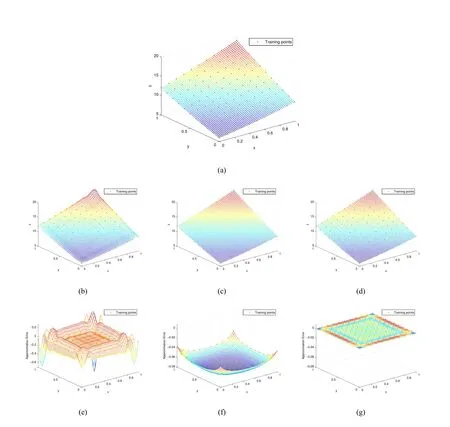
Figure1 Approximating the quadric polynomial surface defined by(2.4)from11×11sampling points.(a)Original surface and training points.(b)and(e)are the reconstructed CSRBF surface and its residual to(a).(c)and(f)are the MMQ-QI surface and its residual to(a).(d)and(g)are our MMQ-CSRBF surface and its corresponding residual to(a).The parameters are set as ρ=0.45 ,c=0.1 2.

3 Shape Preserving Surface Reconstruction

In this section,we will present a two-level fitting method to reconstruct a surface with shape preserving from scattered data.An initial surface is constructed by the MMQ quasi-interpolation formula(2.6),which makes the shape of the surface to be similar with that of the scattered data.RBF-based interpolation is then used to fitting the difference between the initial surface and the scattered data.Shape parameters in the MMQ quasi-interpolation and RBF-based interpolations will be discussed with the shape-preserving property and the approximation capacity.

3.1 Two-level fitting

Surface reconstruction from sampling points discussed here can be stated as follows.For a given(n+1)×(m+1)points setP={xi,yj,zij}(i=0,1,···,n,j=0,1,···,m),a surface can be reconstructed in an implicit way which is to find a functionf(x,y,z)such that its zero level-setS={(x,y,z)|f(x,y,z)=0}passes through the point setP.

RBF-based interpolation is one of the most widely used implicit methods.We can construct a bivariate functiong(x,y)=∑λiϕi(x,y),whereϕiis the basis function,and the coefficientsλican be determined by the constraintsg(xi,yj)=zij.The given pointsPwill exactly locate on the result surfaceS={(x,y,z)|f(x,y,z)=z−g(x,y)=0}.However,as stated in section2.1,this method does not possess the shape preserving property.

Here,we propose a two-level fitting algorithm to solve the shape preserving problem in surface interpolation by combining the CSRBF networks interpolation and the MMQ quasi-interpolation.We first approximate the points setPwith the MMQ quasi-interpolation scheme(2.8)which provides the good shape preserving property,

The approximating error between the surfaces generated by(3.1)and the given dataPcan be described with a bivariate correction function

We adopt a CSRBF networks interpolation to construct the correction function(3.2)under the constraintsh(xi,yj)=zij−(LLf)(xi,yj),i=0,1,2,···,n,j=0,1,2,···,m,as

In the above equation,the first term in the right-hand side gives a base surface for achieving shape preserving.Meanwhile,the second term is for interpolating the given dataPand improving the global approximating accuracy.

The main steps of the shape preserving interpolation algorithm for the given data can be outlined as follows:

Algorithm1.Shape preserving surface reconstruction from the given points.

Input:A set of pointsP.

Output:A surfaceSpassing throughPwith shape preserving properties.

Step1.Construct the MMQ-QI surfaceLLf(x,y)approximating the shape of pointsP.

Step2.Define a correction function(3.2)and compute the correction quantity of the points,hij=h(xi,yj).

Step3.Construct the functionh(x,y)on the data{(xi,yj,hij),i=0,1,···,n,j=0,1,···,m}by using CSRBF networks.

Step4.Obtain the required shape preserving interpolating surface function,z=LLf(x,y)+h(x,y).

3.2 Shape parameters

In the fitting function(3.4 ),there are two shape parameters:the parametercin the MMQ quasi-interpolation and the support sizeρin the CSRBF networks.The accuracy of our two-level fitting depends heavily on the choice of these two parameters.In this subsection,we try to explore the relationship betweencandρ,and provide their heuristic setting for surface approximation with small errors.

As discussed by Floater and Iske[23],the supported radiusρis adjusted to the density of the given points,and it is difficult and time-consuming.To obtain a appropriateρ,we define thek-supported radius of CSRBF.

Definition3.1(k-Supported Radius)Thek-supported radius of CSRBF in the points setPis given as

According to the construction of MMQ basis function(2.5),the smoothing factorcplays an important role in quasi-interpolation.The smallercmakes the quasi-interpolation curves(surfaces,also)closer to the given data.And the biggercmakes the curves further away the given points.Furthermore,from numeric experiments,we found that,for the data with large gradients,the CSRBF-based methods can interpolate the given points exactly,while the errors are large at the other points.In order to obtain an accurate approximation,it is necessary to find a proper smoothing factorcin MMQ quasi-interpolation to generate the error functions with small gradients.

Obviously,the density of the given points is an important factor to determine the parameterc.Here,it can be given as

From(3.5 )and(3.6 ),the problem of determiningcandρis converted into finding two parameterskandh.With a number of numeric experiments,we observed that there existed a function relationship betweenkandhfor achieving a fitting accuracy.The experiments are taken in the following way.

Numeric experiment1

Step1.Sample a surfacef(x,y).The sampling point set is Ω={xi,yj,zij=f(xi,yj),i=0,1,···,an,j=0,1,···,bm},whereaandbare integers.In our experiments,bothaandbare set as5.This set is divided into two subsetsPandQ,whereP={xai,ybj,zai,bj,i=0,1,···,n,j=0,1,···,m}is the training point set for surface fitting,andQ=Ω−Pis for error measuring.

Step2.Fit the data setPwith differentkandh.For each pair of(k,h),a surfaceS(x,y)can be reconstructed from the setP.It is known that too bigkandhwill affect the fitting efficiency and accuracy.Here,we setkas the integer numbers in the interval(0,120],andhas the values of 101uniform samples in the interval[0,10].So,for each data setP,120×101surfaces are generated.

Step3.Compute the approximation errors with the data setQ.The approximation error is defined as

whereDis the domain of the surfacef(x,y).For each fitting surfaceSk,h(x,y)with the specifiedkandh,the approximation errorek,his computed by the setQ.We denote the minimum of the approximation errors with all pairs(k,h)asemin.

Step4.Construct the valid intervals ofh.We use a ratee/eminto measure the fitting accuracy of a surface with the specifiedkandh.Then,all validhs can be found for eachkwhen the ratee/eminof a fitting surface is less than the given error thresholdηe.Thesehs form a set in which the minimal one and the maximal one are the bounds of a interval[hLB,hUB].Fig.2shows the intervals ofhunder different precision thresholdsηe=20,15,and5,where the surface is the quadratic polynomial surface in Fig.1(a).As the precision of the approximation increases,the interval ofhgets shorter for a fixedk.The same phenomenon happens in other surface approximation cases.

Whenηeis traversed from1to100,we do the above steps for surfaces with different sizes of the fitting setP,such as Quadric polynomial surface(11×11),Quadrical polynomial surface(21×21),Cubic polynomial surface(11×11),Sine polynomial surface(11×11),Arc surface(11×11),Peaks(part)(11×11),Peaks(part)(21×21),where all surfaces are defined in the next section,except for the quadric polynomial surface which is defined in subsection2.1,and combine all valid intervals ofhtogether,see Fig.3(a).

In CSRBF methods,too smallkwill lead the domain of the surface to be uncovered by influences of the RBF centers,while too bigkwill increase the complexity and the instability.In our paper,k∈[4,35]can work well for all sampling points.Fig.3(b)extracted from Fig.3(a)shows the intervals ofhwithk∈[4,35].It is observed that there is a narrow band where the upper bounds and lower bounds are mixed.The mixed band illustrates a relationship ofk-hunder a acceptable precision.Fig.3(c)shows a quadratic polynomial curve which is used to fit the relationship ofk-hin the band,

Figure2 Relationship between the interval of the right h and k under a given precision threshold ηe for quadratic polynomial surface(2.4)

Figure3 Construction of the functional relationship between h and k by all the experiments in Table2with ηe traversing from1to100.(a)The upper bounds and lower bounds of h for all experiments with all ηe.(b)The part of(a)where k∈[4,35].(c)The fitting curve between h and k in the narrow band formed by the mixed upper bounds and lower bounds of h.

With(3.8),the correspondinghis obtained for eachk∈[4,35].In Table2,for seven data sets,we list the maximal errorse1,the minimal errorse2,and the values of their corresponding(h1,k1)and(h2,k2).Errorse3are also listed in Table2,which is the minimal approximation errors for allk∈(0,120]and allh∈[0,10].Actually,his set as one of the101uniform samples in the interval[0,10].From Table2,it is exciting that(3.8)can provide a good choice ofhwith respect to anyk∈[4,35]for fitting a surface with a small approximation error.And in interval[4,35],the biggerk,the smaller approximation error.

Table2Analysis of approximation accuracy

4 Numerical Examples

In this section,several results are provided to illustrate the effectiveness of the proposed algorithm for shape preserving surface approximation,where the residuals are the errors in the whole domain of a surface,not only on the training points.Especially,the residuals on the training points are almost zero,because the method interpolates those points.If without considering the round-off error,they are exactly equal to zero.Given the approximated functionf(x,y),the residual function could be defined as follows

whereS(x,y)denotes the approximation surface,and(x,y)∈Df,the domain of the functionf(x,y).

In all Examples(Example4.1 -4.5 )in this section,the training points are taken from the samples of the surface,and the testing set are5times more dense than the training set in each direction.Due to the density of the training points,the parametersρandcare not the same for different samples.In the fitting procedure,the parameterkcan be selected randomly in the interval[4,35].Here,kis set as20for all examples and works well.The parameterhis computed with(3.8),soh=1.2.The fixedkandhare beneficial to study the robustness of the parameters setting in the proposed method.

In each example,the results of the CSRBF networks interpolation(2.1),the MMQ quasi-interpolation(2.8 )and our proposed method(3.4 )are compared with each other.Figs.4-10show seven examples.Each result includes the original surface,the training points for surface fitting,three reconstructed surfaces with three different methods and their corresponding residuals to the original surface.Their approximation errors are listed in Table3.From the Figs.4-10and Table3,it is easy to find that our MMQ-CSRBF method can reconstruct shape-preserving surfaces with high accuracy.

Table3Approximation error statistics

Example4.1(Quadric Polynomial Surface)The point setPis obtained by sampling the quadric polynomial surface(2.4)with21×21training points.According to Figs.4(d)and4(g),it is obviously that MMQ-CSRBF approximates the quadric polynomial surface well.Like MMQ-CSRBF,MMQ-QI reconstructs the surface with shape preserving(Fig.4(c)),but its approximation error(e=2.434 e-2)is bigger than MMQ-CSRBF(e=1.608 e-4).Figs.4(b)and4(e)show the CSRBF networks leads to a non-shape preserving and overfitting surface.Moreover,the variance in Table3indicates the stability of the proposed MMQ-CSRBF method.

Compared with the surface approximated by using11×11sampling points in subsection2.1,MMQ-CSRBF stands out in the three methods with the samekandhfor different density sampling points.On the other hand,the approximation accuracy of MMQ-CSRBF with11×11sampling points(3.552 e-4 in Table1)is still several orders of magnitude better than the other two methods with21×21sampling points(CSRBF:1.080 e-0and MMQ-QI:2.434 e-2in Table3).

Example4.2(Cubic Polynomial Surface)The training point setPis formed by sampling11×11 points on a cubic polynomial surface

From the setP,three surfaces reconstructed by three methods are shown in Fig.5.Figs.5(b)and5(e)demonstrate that the CSRBF interpolation surfaces are the worst for their largest approximation errors and big deformations near the boundaries.Fig.5(c)indicates the MMQ-QI only approximates the surface with shape preserving,and the residual errors are larger than the MMQ-CSRBF(Fig.5(f)).As expected,Figs.5(d)and5(g)show that the MMQ-CSRBF approximates the cubic polynomial surface very well,and the residuals listed in Table3show that the MMQ-CSRBF is the highest accurate and most stable method to approximate the cubic polynomial surface.

Example4.3(Sine Polynomial Surface)The sine polynomial surface

is sampled into11×11points as the training points for surface fitting.From the points,three reconstructed surfaces are displayed in Fig.6.Fig.6(c)indicates that there are many sampling points are away the MMQ-QI approximation surface,and Fig.6(f)shows the residual errors are big.Although Figs.6(b)and 6(e)demonstrate that the CSRBF performs better than the MMQ-QI,the residual errors of the CSRBF networks surface are still large.Figs.6(d)and6(g)show our MMQ-CSRBF method can approximate the sine polynomial surface very well.The residuals in Table3could verify this.

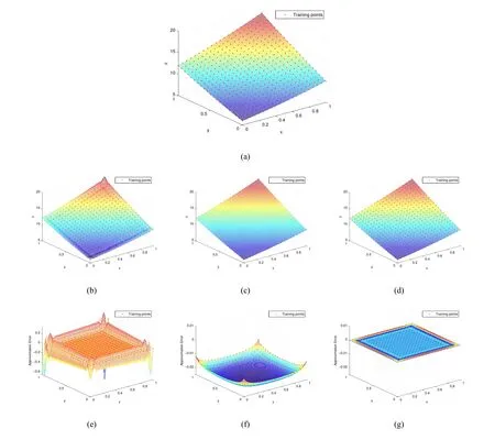
Figure4 Surfaces reconstructed from21×21points sampled on the quadric polynomial surfaces(2.4).(a)The original surface and training points.(b)-(d)and(e)-(g)are the surfaces and their residuals to(a)using three methods,CSRBF,MMQ-QI,and MMQ-CSRBF,respectively.The parameters are set as ρ=0.22 (k=20)and c=0.06 (h=1.2).

Example4.4(Arc Surface)Given a points setPwith11×11training points sampled on the arc surface

three surfaces are reconstructed by three methods for comparison,as shown in Fig.7.From the fitting results in Fig.7and the approximation errors in Table3,these three approximation surfaces are not fitted well.That maybe because the samples on the Arc surface are very non-uniformly distributed,especially near the boundaries.

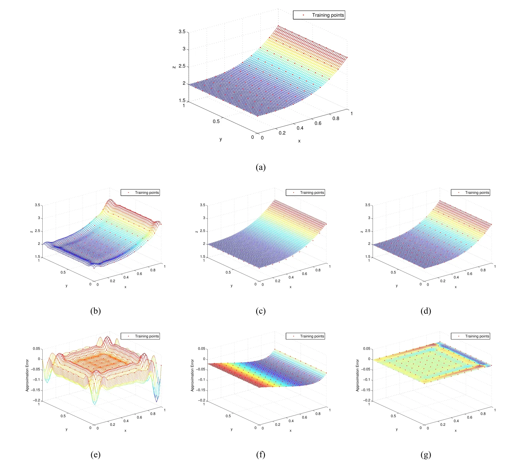
Figure5 Comparisons of reconstructed surfaces by three different methods.(a)The cubic polynomial surface and 11×11training points.(b)and(e)are the result surface by CSRBF and its residual to(a).(c)and(f)are for MMQ-QI.(d)and(g)are for MMQ-CSRBF.All results are generated by the same parameter setting as ρ=0.45 (k=20)and c=0.12 (h=1.2 ).

Example4.5(Peaks Surface)Given the peaks surface

in order to show the performance of the proposed method approximating the surface with different density,we sample two training points sets on the part of the surface(4.5),wherex,y∈[0,1]×[1,2].LetP11denote the set with11×11sampling points,andP21the set with21×21sampling points,the approximation surfaces can be generated by the three methods from the two training point sets.From Table3,Fig.8and Fig.9,it obviously shows that any one of the surfaces reconstructed by the MMQ-CSRBF is significantly better than the surfaces generated by the other two methods.

Figure6 Comparisons among the reconstructed surfaces by three methods from a point set with11×11points sampled on a sine polynomial surface(4.3).(a)the original surface and training points.(b),(c),and(d)are the surfaces generated by CSRBF,MMQ-QI,and MMQ-CSRBF,respectively,with same parameter setting ρ=0.45 (k=20)and c=0.12 (h=1.2 ).(e),(f),and(g)are their corresponding residuals to(a).

Moreover,if we expand the fitting domain up to36times,e.g.x,y∈[−3,3]×[−3,3],and the number of the sampling points goes up to31×31,Fig.10shows that the MMQ-CSRBF can still reconstruct the best approximation surface among the three methods.Their approximation errors can be checked in Table 3.

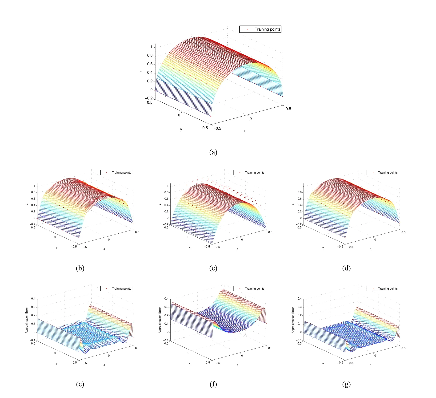
Figure7 Approximations of the arc surface(4.4)with three methods from11×11training points.(a)is the original surface and training points.(b)-(d)are the approximating surfaces with methods CSRBF,MMQ-QI,and MMQ-CSRBF.(e)-(g)are the residuals of(b)-(d)to(a),respectively.All results are generated by using the same parameter setting ρ=0.45 (k=20)and c=0.12 (h=1.2 ).

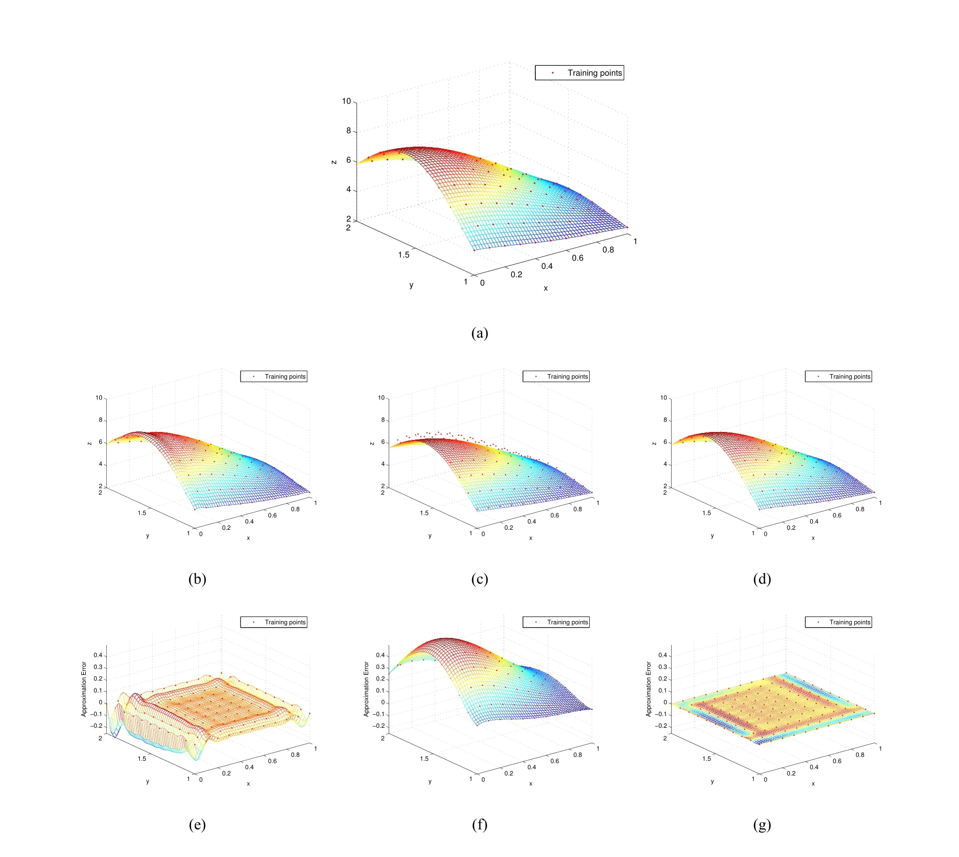
Figure8 Comparison of the three approximate surfaces by different methods(CSRBF,MMQ-QI,and MMQ-CSRBF).(a)The original surface which is one part of the peaks surface(4.5),with11×11training points on it.The second row includes the surfaces by the three methods,(b)CSRBF,(c)MMQ-QI,and(d)MMQ-CSRBF.The third row shows their corresponding residuals to the original surface(a).All methods adopt the same parameter setting,ρ=0.50 (k=20),c=0.12 (h=1.2 ).

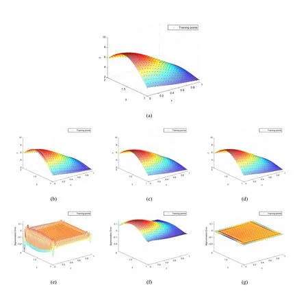
Figure9 Comparison of the three approximate surfaces by different methods(CSRBF,MMQ-QI,and MMQ-CSRBF).(a)The original surface which is one part of the peaks surface(4.5),with21×21training points on it.The second row gives the surfaces by the three methods,(b)CSRBF,(c)MMQ-QI,and(d)MMQ-CSRBF.The third row shows their corresponding residuals to the original surface(a).All methods use the same parameter setting,ρ=0.22 (k=20),c=0.06 (h=1.2 ).

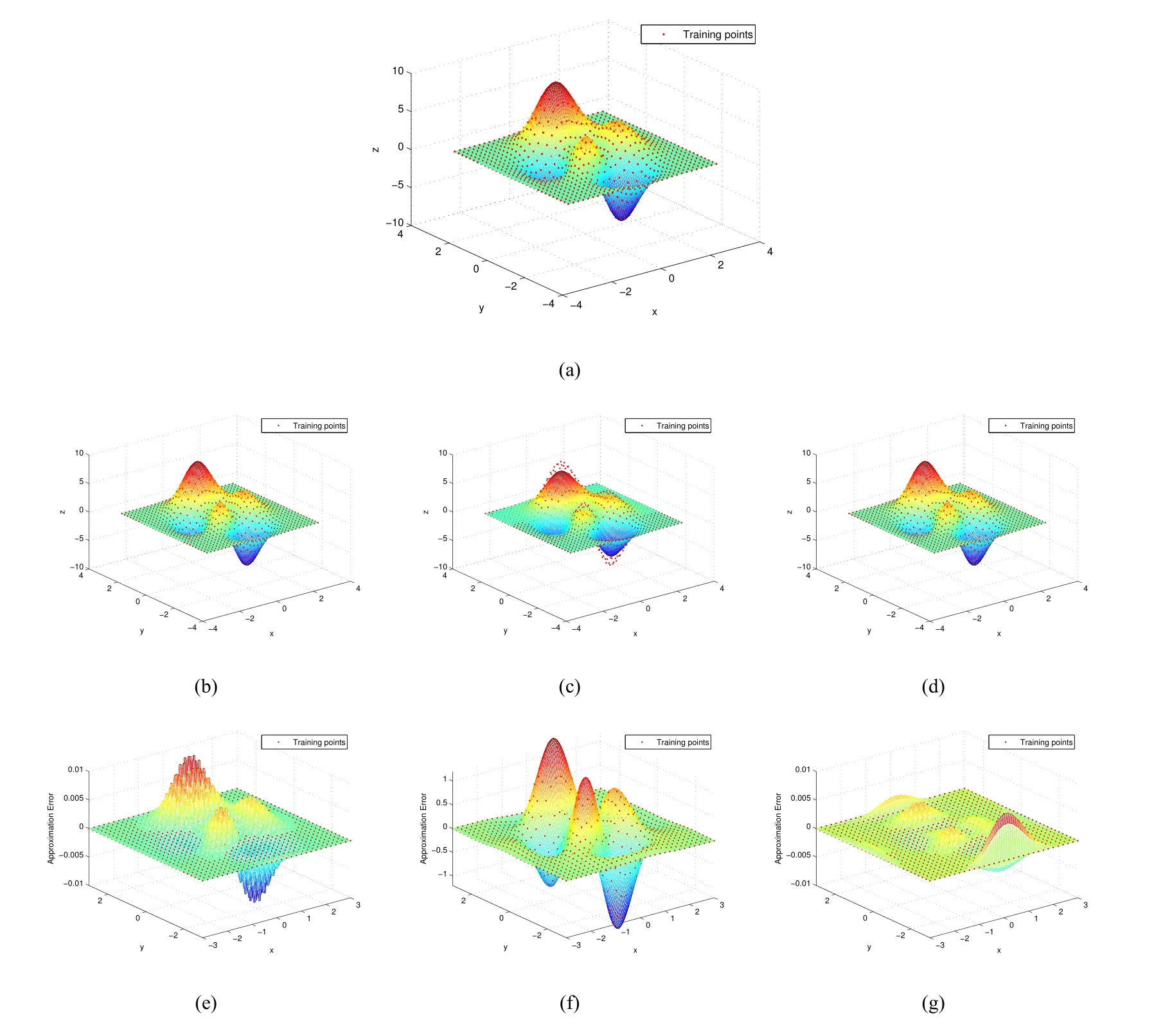
Figure10 Comparison of the three approximate surfaces by different methods(CSRBF,MMQ-QI,and MMQ-CSRBF).(a)The original peaks surface(4.5)with31×31training points on it.The surfaces shown in the second row are generated by the methods,(b)CSRBF,(c)MMQ-QI,and(d)MMQ-CSRBF,respedtinely.The third row shows their corresponding residuals to the original surface(a).The three surfaces are generated by using the same parameter setting,ρ=0.89 (k=20),c=0.24 (h=1.2 ).

5 Conclusions

The RBF-based interpolation methods are an important class of surface approximation methods[7,8,9,10,11,12,13].However,they suffer from the efficiency and the non shape-preserving property which limit them to be used widely for the large scale data.Although using CSRBFs[6]can improve the fitting efficiency,the surface reconstructed by them is still not shape-preserving.The MMQ quasi-interpolation method[19,20,21]is a shape-preserving surface fitting method,while the parametercis hardly chosen to balance the smoothness and the accuracy.In this paper,a two-level fit method is proposed to fitting a shape-preserving surface with a high accuracy from the given data,by combining the MMQ quasi-interpolation method and the CSRBF-based method.An initial surface is first constructed by the MMQ quasi-interpolation method,which is shape-preserving,and then a CSRBF networks fitting process is performed to improve the fitting accuracy.In addition,a function betweenhandkfor determining the values of parameterscandρis created to generate a fitting surface with a small approximation error by a number of numerical experiments,wherek∈[4,35],with balancing the efficiency and the accuracy.It simplifies the setting of parameterscandρ,and benefits the users without experiences in shape designing.