Impact of COVID-19 pandemic on stock market via sparse principal component analysis

Li Ming, Wen Canhong

Department of Statistics and Finance, School of Management, University of Science and Technology of China, Hefei 230026, China

Abstract: The COVID-19 pandemic has caused severe public health and economic consequences around the world. It is of great importance to evaluate the impact of the COVID-19 pandemic on the economy, especially the stock market. To this end, we proposed to use several state-of-art sparse principal component analysis (PCA) methods for the stock data of the CSI 300 index from February 1, 2019 to February 1, 2021. To show the influence of the outbreak of the COVID-19 pandemic, we divide this period into two periods, i.e., before and after January 1, 2020. Based on this division, we attempted to extract the principal components and construct portfolio accordingly. The results show that the proportion of principal components representing the market declined after the outbreak. For the constitution in the first two principal components, the important stock sets are substantially different after the outbreak. The stocks from the health care sector start to play an important role in the portfolio of the CSI 300 index after the outbreak. Compared with the CSI 300 index, the first two principal components from the sparse PCA methods can obtain higher returns with a much smaller set of stocks in the portfolio. In conclusion, the outbreak of the COVID-19 pandemic led to changes in both proportion and constitution of the principal component of the stocks in the CSI 300 index.

Keywords: COVID-19 pandemic ; sparse PCA; stock index

1 Introduction

1.1 Background and data description

The COVID-19 pandemic from the end of 2019 not only poses a serious threat to human life and health, but also causes major losses to the global economy. In order to control the pandemic, quarantine measures have been gradually adopted around the world, some economies have been temporarily shut down, and financial markets have also fallen into a state of continuous decline. As known, the stock market is a barometer of the economy. The stock price not only fluctuates with changes in the economic cycle, but also indicates the economic development situation, and its fluctuations may lead to a recession in the real economy. For example, after the outbreak of the COVID-19 pandemic, on the first day of the opening of the Shanghai and Shenzhen markets, 3188 stocks in the two markets fell by their limit.

Figure 1 shows the CSI 300 index, an index compiled from the most representative 300 stocks in Shanghai and Shenzhen A-shares with large scale and good liquidity. It can be seen that it dropped down 7.88% on February 3, 2020, and experienced several major fluctuations during the COVID-19 pandemic period.

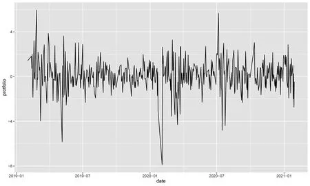
Figure 1. The CSI 300 index portfolio from January 1, 2019 to February 1, 2021.

It is of great interest to to evaluate the impact of the COVID-19 pandemic on the Chinese stock market, especially the CSI 300 index, one of the most important benchmarks in the A-share market. However, the CSI 300 index contains 300 stocks from various fields, and the correlation between them is complicated, so it is difficult to analyze them. Thus it is essential to perform some dimension reduction to the 300 stocks and find out the difference before and after the outbreak of the COVID-19 pandemic.

1.2 Literature review

Principal component analysis (PCA) is one of the most popular technique to reduce the dimension, and has been well studied in the fields of statistics and finance, such as portfolio management[1]. By converting stocks into a new set of uncorrelated principal components that represent uncorrelated risk sources, PCA can reduce the complexity of stock portfolios. PCA allows us to determine the stocks that can be used as a representative of the entire data set, thereby finding the number of stocks that are sufficient to diversify the portfolio.

Due to the large number of stocks, the principal components (PCs) derived from PCA consist of all stocks and it is hard to explain the effect of each stock. To address this issue, sparse version of PCA has been proposed by controlling the number of the variables in the PCs.

The first class of approaches are based on ad-hoc methods by post-processing the PCs obtained from the standard PCA. For example, Cadima and Jolliffe[2]proposed a simple thresholding approach by artificially setting the loadings with absolute values smaller than a threshold to zero. Vines[3]considered simple principal components by restricting the loadings to take values from a small set of allowable integers such as 0, 1, and -1. Although these methods are simple to operate, the sparse PCs obtained usually have large errors. In 2013, Ma[4]proposed an iterative thresholding sparse PCA algorithm based on the QR decomposition. It overcomes the drawbacks of simple thresholding by iterative update, and thus has better performance in both theory and numerical experiment. As the authors stated, however, the convergence of the algorithm is not guaranteed.

In recent years, more involved approaches have been presented. These methods usually impose regularization on different PCA formulations. A classic perspective is that PCA finds a set of directions (technically, a linear subspace) that maximizes the variance of the data once it is projected into that space.Jolliffe et al.[5]developed the Simplified Component Technique-LASSO (SCoTLASS) algorithm for finding sparse orthogonal loading vectors by sequentially maximizing the approximate variance explained by each PC under thel1-norm penalty on loading vectors.d’Aspremont et al.[6]proposed a direct sparse PCA (DSPCA) method, to obtain sparse PCs by solving a sequence of semi-definite program relaxations. In 2008, Journée et al.[7]formulated the sparse PCA problem as a nonconcave maximization problem withl0-norm orl1-norm sparsity-inducing penalties. They showed that the problem can be reduced into maximization of a convex function on a compact set, and developed a computationally efficient gradient method for finding a stationary point. Inspired by the greedy method for solving the combinatorial problem[8], d’Aspremont et al.[9]proposed a greedy heuristic algorithm to solve a new sparse PCA semi-definite programming problem. In 2013, Croux et al.[10]proposed to use a grid search algorithm to derive a sparse version of PCs and achieved desirable results. The eigen decomposition formulation of PCA also relates PCA to the singular value decomposition (SVD) of data matrix. Shen and Huang[11]used SVD to calculate the low-rank matrix approximation of the data matrix under various sparsity-inducing penalties, and applied it to the sparse PCA problems (sPCA-rSVD). This method uses least squares linear regression and simple threshold rules, so it is relatively easy to implement.

Alternatively, the PCs can be interpreted in geometric as the closest linear manifold approximation to the observed data.Based on this, Zou et al.[12]formulated the sparse PCA problem as a regression-type optimization problem and imposed constraint on the coefficients via a combination ofl1- andl2-norm penalties.PCA can be also reformulated as a maximum likelihood solution to a latent variable model, called probabilistic PCA[13]. For example, Sigg and Buhmann[14]modified the expectation maximization approach of probabilistic PCA to encourage sparsity or non-negativity to the loading factors.

In this article, we aim to investigate the structural changes of the index stocks before and after the outbreak of the COVID-19 pandemic. To this end, we collect the constituent stock data in the CSI 300 index from the Wind database (http://www.wind.com.cn/), and propose to apply sparse PCA techniques as well as the classic PCA method to the index stocks data. We also examine the performance of different sparse PCA methods in extensive simulated data.

The structure of the remaining contents is as follows. Section 2 introduces several commonly used sparse PCA methods. Section 3 shows the analysis on CSI 300 constituent stock data via PCA and sparse PCA technique. In Section 4, numerical experiments are carried out on several commonly used sparse PCA algorithms. We conclude with a short discussion in Section 5.

2 Algorithms for the sparse PCA problem

In this section, we review four popular sparse PCA methods, which include the variance maximization (VM)[10], the reconstruction error minimization (REM)[12], the singular value decomposition (SVD)[11]and the probabilistic model (PM)[14]. Table 1 gives a brief summary on the four methods, and we will discuss them in details in the afterward sections.

2.1 Variance maximization (VM)

The variance maximization approach was proposed by Croux et al.[10]. The main idea is to preserve as many changes in the original sample as possible when projecting data points into a low-dimensional space.Note that maximizing the variance of the first PCXv1can be equivalently expressed as

(1)

Based on this formulation, Croux et al.[10]introduced a sparse PCA framework by imposing al1penalty function into the objective function of (1), that is

(2)

whereλ1(≥0) is a regularization parameter that controls the amount of shrinkage on the first PC. It can be seen that the larger the value ofλ1, the greater the amount of shrinkage (i.e. the greater the amount of zero estimates). Then based on the top (j-1)-th PCs, thej-th sparse PCs can be solved via the following optimization problem:

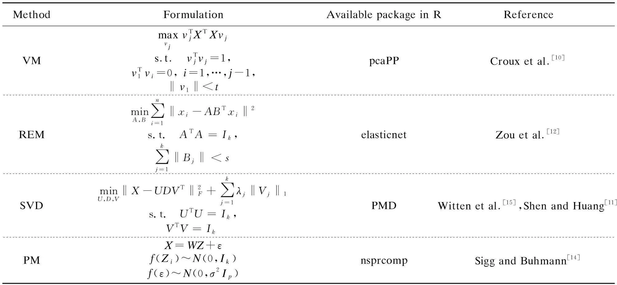
Table 1. Summary of sparse PCAs: VM, REM, SVD, and PM.

vTvj-1=0

(3)

whereλj(≥0) is a regularization parameter that controls the amount of shrinkage on the firstj-th PC.

Since the principal components are required to be orthogonal,j-1 constraints are added for solving thej-th PC, which makes the problem (3) difficult to solve. Croux et al.[10]proposed to use a grid search algorithm to obtain the PCs, and showed that it is very fast and has a high accuracy in the high-dimensional setting. The basic idea of the algorithm is to simplify the problem into a series of optimizations in a two-dimensional plane under the constraint of unit norm. This boils down to a series of maximization of functions on the unit circle. This is simply a univariate maximization problem, which can be solved by a grid search.

(4)

The grid search algorithm for the variance minimization problem (4) is given by the following algorithm.

Algorithm 2.1The variance minimization approach via grid search algorithm

1. Sort the columns ofX(j)in descending order of variance. Then the first variable has the maximum variance value, and its corresponding loading vectorv=(1,0,…,0) is used as the first approximation of the solution, where the length ofvisp-j+1.

2. Forl=1,2,…,m, using the iterative steps to update all the components of the vectorv: For 1≤i≤p-j+1, update thei-th componentviof the current best approximationv, which is achieved by maximizing the following equation to findγ*:

f(v1b(γ),…,vi-1b(γ),cosγ,vi+1b(γ),…,vp-j+1b(γ)),

2.2 Reconstruction error minimization (REM)

While the VM approach obtains the PCs by maximizing the variance, we can also derive the PCs via minimizing the distance between projected data and the original ones. As described in Reference [16], this method can be formulated as follows,

s.t.VTV=Ik

(5)

Inspired by this formulation, Zou et al.[12]reconstructed the product of the loading matrix,VTV, into twop×kmatricesATB. Based on this reconstruction, they proposed a sparse PCA method by adding a combination ofl1andl2penalties toBand leaving the orthogonal constraint toA, that is,

s.t.ATA=Ik

(6)

whereβjis thej-th column ofB,λis a parameter controlling the norm of loading vectors, andλ1,jis a parameter that controls the sparsity of the load vectorβj. For data set withn>p, assume thatλ>0, and for data set withn≤p,λ=0.

The REM approach links the estimation of sparse PCs with variable selection in linear regression. When fixing the matrixA, solving the problem with respect toBis an elastic net problem, which has be well studied, see Reference [17] for example. Based on this, Zou et al.[12]developed the block coordinate descent algorithm to the REM approach by optimizing the variables of (5), i.e.,AandB, in two separate sub-problems. The detail algorithm is presented as follows.

Algorithm 2.2The REM approach via bolck coordinate descent method

1. LetAbe initialized toV[,1:k], which is the load of the firstkordinary principal components.

2. For a givenA=[α1,…,αk], forj=1,2,…,k, solve the following elastic network problem:

3. For a givenB=[β1,…,βk], calculate the SVD decompositionXTXB=UDVT, and then updateA=UVT.

4. Repeat Steps 2,3 until convergence.

As described in Reference [12], the empirical evidence shows that the output result of the algorithm does not change much with the change ofλ. For the case ofn>p, the default termλcan be zero. In fact,λusually takes a small positive number to overcome the potential collinearity problem ofλ.

2.3 Singular value decomposition (SVD)

An alternative way to obtain the loading matrix productVTVis by using the singular value decomposition (SVD).Mathematically, let the SVD ofXbeX=UDVT, whereU=[u1,…,ur] with orthogonal columns,V=[v1,…,vr] with orthogonal columns, andD=diag{d1，…,dr} withd1≥…≥dr. It can be easily to see that thej-th loading vector ofXTXisvj,j=1,…,r. Thus we can obtain the PCs ofXTXby performing SVD to matrixX.

(7)

is

(8)

(9)

The above discussion are summarized as follows.

Algorithm 2.3The SVD approach via iterative method

2. Update:

3. Repeat Step 2 until convergence.

It can be seen that Algorithm 2.3 only contains simple linear iteration and group reduction rules. Therefore, it has the advantages of easy implementation and high computational efficiency.

2.4 Probabilistic model (PM)

Sigg and Buhmann[14]showed that the PCs can also be redefined as the maximum likelihood solution of a probabilistic latent variable model. The original data is assumed to be

X=ZW+ε

(10)

whereZ={Z1,…,Zn}Tis the latent variable,W∈k×prepresents the principal component, its row vector is regarded as ak-dimensional latent variable,is the noise. Both the latent variable and noise are assumed to follow the normal distribution, that is,Zi～N(0,Ik),ε～N(0,σ2Ip). Then, the marginal distribution ofXis a normal distribution with a mean value of 0 and a variance ofWTW+σ2Ip. The estimation of the parametersWandσ2can be achieved by the maximum likelihood function. Sigg and Buhmann[14]proposed using the variational maximum expectation algorithm to estimate the parameters.

To obtain sparse PCs, we add a step of axis-aligned gradient descent to the probabilistic model, and the detailed algorithm is presented as follows:

Algorithm 2.4The PM approach via gradient descent method

1. Initializet=1, apply standard SVD procedure toX, and then get the first principal component ofXasW(t).

(1)y=XW(t);

Figure 2. Cumulative returns of the stocks in the CSI 300 index from February 1, 2019 to February 1, 2021.

(4)fork=1,…,K, add (sk-sk+1) to the 1,…,kelements ofX(t+1);

(5)rearrange the elements inW(t+1)according toπ,t=t+1.

3. OutputW.

3 Empirical analysis

3.1 Data exhibition

We investigate the performance of the classic PCA and the sparse PCA methods described in Section 2 to the stock data from February 1, 2019 to February 1, 2021. We obtained the daily yield of the 234 unique stocks in the CSI 300 index from the Wind database. Figure 2 shows the cumulative daily return of 234 stocks in CSI 300 since February 1， 2019. It can be seen that some stocks are showing a clear upward trend, while others are showing a downward trend.

We define the sectors as General Industry Classification groups (GICs)[18], see Table 2.

3.2 Results from PCA

We first divide the whole period into two non-overlap periods: ①the period before the outbreak of the COVID-19 pandemic: from February 1, 2019 to December 31, 2019; ②the period after the outbreak: from January 1, 2020 to February 1, 2021.

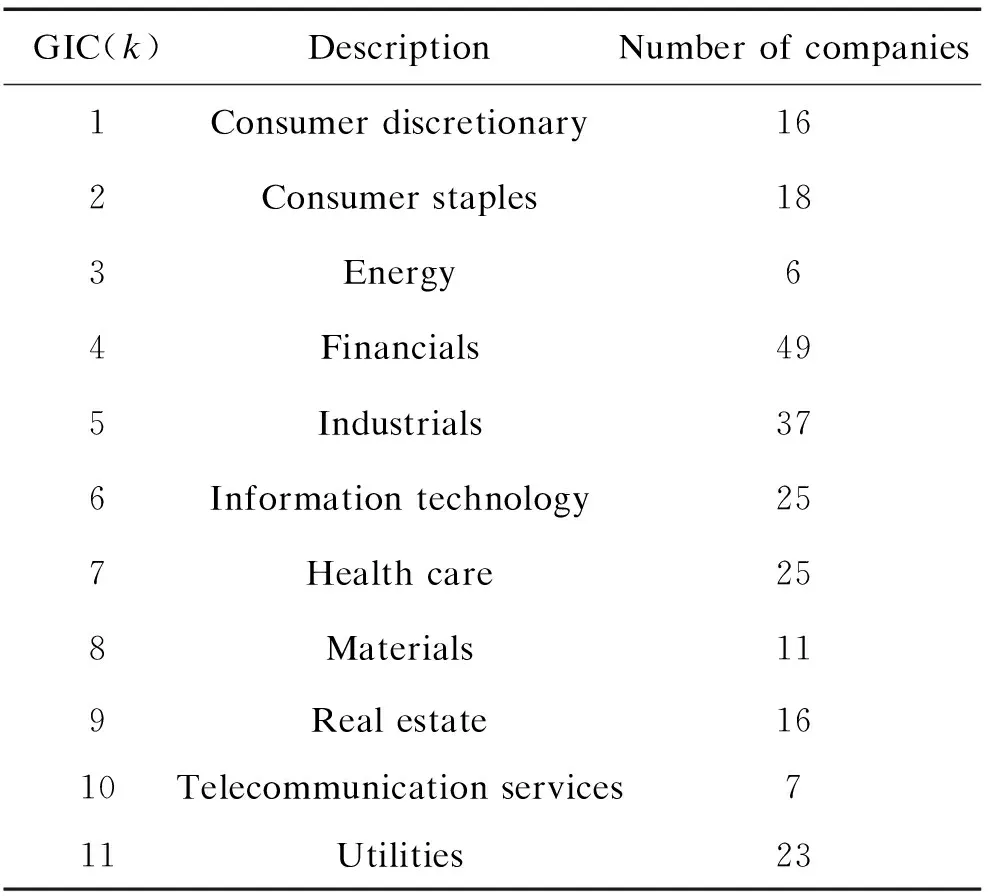
Table 2. General Industry Classification (GIC) sectors.

Figure 3 shows the first five principal components calculated from PCA before and after the outbreak. It can be seen that in 2019, the first PC has a large variance, about 37.4%, followed by 5.2%, 4.8%, 2.3% and 2.2%.

In comparison, after the outbreak, there is an obvious increment in the variance value of the second PC, while the variance of the first PC drops down to 33.6%. It suggests that the second PC absorbed some variations from the first PC after the outbreak. To provide further insight into the impact of the pandemic, let us look at the factor loading graph on the right panels in Figure 3. While the first PC has a similar coefficient values in most stocks, yet the directions of factor loadings in the second PC change substantially after the outbreak.

Figure 3. The first five PCs from classic PCA before and after the outbreak of the COVID-19 pandemic.

As known, the first PC represents a linear combination of input data that explains most of the differences. It turns out that this is the “market factor”, i.e., the trend of securities to rise and fall together as an asset class. The right panel of Figure 3 illustrates this by showing that all stocks have the same sign on the first PC. In other words, it is empirically the case that there is a dominant systematic factor called the equity risk premium explaining the variance of returns. This is because macro variables, such as monetary, fiscal policy, growth expectations, political risk, regulatory risk and other factors, influence the returns of all stocks.

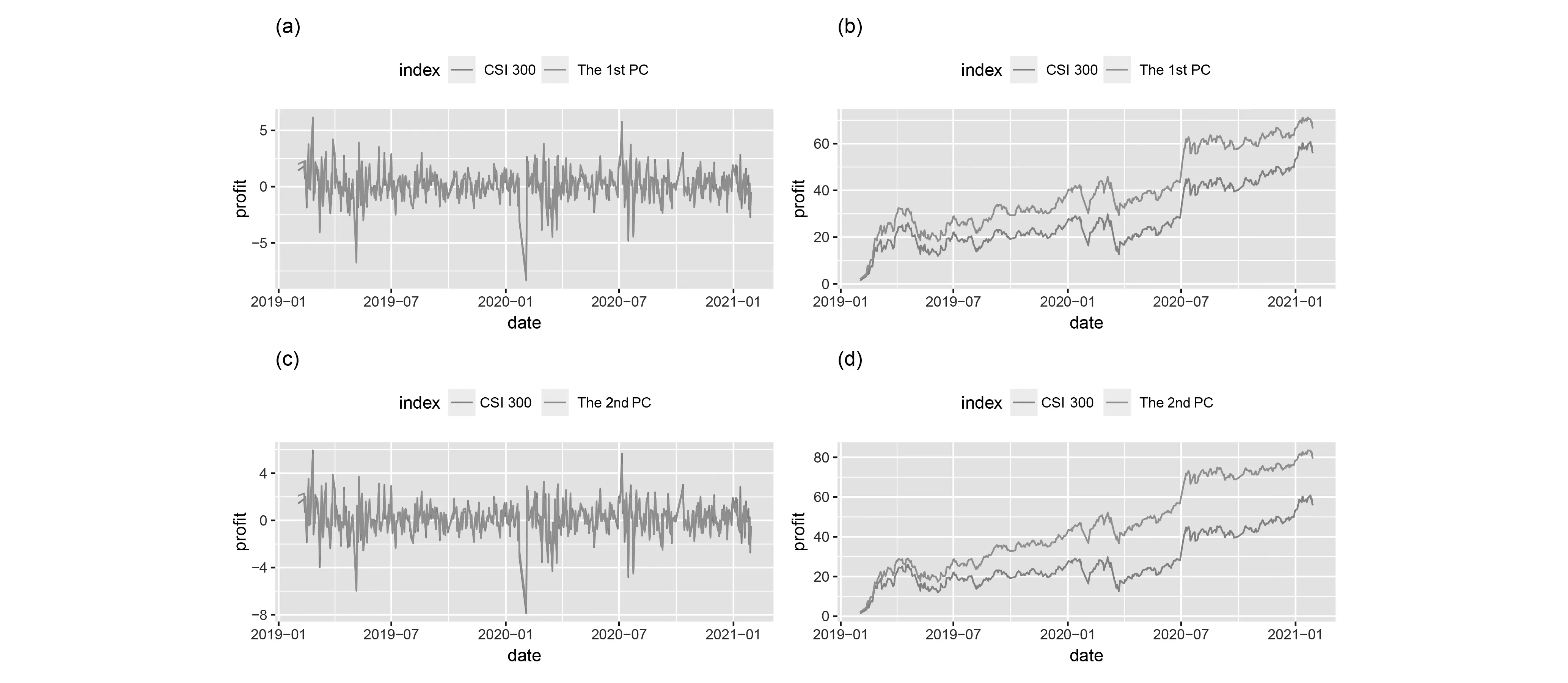
Figure 4. Portfolio for the stocks from the first two PCs. The CSI 300 index is also included for comparison. The daily and cumulative portfolios are presented in the left and right panels, respectively.

Figure 4 plots the return of the investment portfolio based on the first and second principal components and the CSI 300 index. It can be seen that both the portfolios from the first and second PCs have higher cumulative returns than the CSI 300 index. Furthermore, the portfolio returns of these two PCs are similar in 2019, but after January 1， 2020, the total returns of the portfolio of the second PC is significantly higher than those of the first PC. This might be due to that the sudden outbreak led to high demand in certain areas, which resulted in the growth of stocks in those fields. We will explore this furthermore via sparse PCA technique.

Figure 5 shows the daily profit by zooming in the top left panel of Figure 4 during the period of January 1, 2020 and April 20, 2020. In addition, the number of new domestic cases is included for comparison. We divide this period into five stages according to the portfolio changes.

(Ⅰ) The first stage (before January 9, 2020): The stock price fluctuates steadily, and there is no obvious upward or downward trend. At this time, news of “unexplained pneumonia” was only spread in a small area and had not attract the attention of the government and the public, so it had no obvious impact on the stock market.

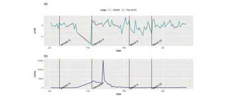
Figure 5. Portfolio for the stocks from the first PC and the CSI 300 index from January 1, 2020 to April 20, 2020. The number of new domestic cases is included in the bottom panel. The vertical black line indicates the division of five stages, which are defined by the portfolio changes.

(Ⅱ) The second stage (January 9, 2020 to February 3, 2020): On January 9, the expert evaluation team of the National Health Commission released information on the pathogen of Wuhan’s unexplained virus pneumonia and determined that the pathogen was a new type of coronavirus. Based on the fear of SARS, a coronavirus in 2003, the public panicked and began to stock up large amounts of medical supplies such as masks and disinfectants. On January 23, 2020, Wuhan and several cities in Hubei issued the “lockdown” rule. At the time of the Lunar New Year, the population movement was large, which caused the pandemic to spread to a certain extent across the country. The entire Spring Festival is the most severe period of the pandemic, and the surge in the number of confirmed cases continues to challenge the public confidence. Since the market is closed during the Spring Festival, the CSI 300 index fell by 8% on the first day of opening after the Spring Festival. Although the pandemic did not spread across the country, the CSI 300 index showed a volatile decline.

(Ⅲ) The third stage (February 4, 2020 to March 5, 2020): On February 3, Wuhan Huoshenshan Hospital received the first batch of patients. The P3 Laboratory in Zhejiang Province has isolated 8 strains of viruses, several of which are very suitable for vaccines.At the same time, with the unfolding of the anti-pandemic, the number of newly diagnosed patients has begun to decline, and public confidence has been greatly improved. The stock market has shown an upward trend amidst volatility.

(Ⅳ) The fourth stage (March 5, 2020 to March 23, 2020): On March, the pandemic in China was basically under control, but overseas pandemic s began to break out, and U.S. stocks experienced four circuit breakers. Affected by the U.S. stock market, the domestic stock market experienced a major decline.

(Ⅴ) The fifth stage (March 23, 2020 to April 20, 2020): In the second half of March, domestic confirmed diagnoses are basically cleared. With the resumption of work and production on a large scale, the stock market began to pick up and gradually returned to the average line before the pandemic.

(Ⅵ) The sixth stage (after April 20, 2020): Starting from the second half of April, the domestic pandemic has been well controlled, and the order of production and life before the pandemic has been completely restored. The stock market has also returned to a state of steady volatility before the pandemic. However, after experiencing such a rapid and powerful pandemic, the structure of the stock market in the post-pandemic era requires further analysis.

3.3 Results from the sparse PCA methods

The results from PCA shows how the pandemic influences the stock market. Next we will present more difference before and after the outbreak, especially the difference in the leading stocks set. We fix the number of the first and second PCs to be 10, and perform four sparse PCA methods mentioned in Section 2 on the stock data. We also include the simple truncating (ST)[2]method by keeping the top 10 elements of PCs (in absolute value) from the classic PCA method and truncating the remaining elements to be zero.

First of all, we applied all the above methods to the entire period. Table 3 shows the GIC of the nonzero elements in the first two sparse PCs. It can be seen that the stocks selected by the first PC mainly belong to the financial field, while those of the second PC mainly belong to the health care or industrial field except for the PM approach. We will provide further insight into it by separating the period by the outbreak.

Figure 6 and Figure 7 present the selected stocks in the first two PCs for the periods before and after the outbreak, respectively. The stocks are arranged according to the absolute value of the loadings. We also include the GIC sector that the stocks belong to in Table 4 and Table 5. It can be seen that before the outbreak, the stocks in the first PC are mostly from financial field for all methods except the VM method. Different from other methods, both the two PCs from VM have complicate constructions. For the second PC, both REM and SVD yields to a combination of industrial stocks. The second PC of PM methods still consists of financial stocks.

Table 3. The nonzero loading fields from different sparse PCA techniques on entire period.

Figure 6. The selected stocks in the first two PCs for the periods before the outbreak of the COVID-19 pandemic. The stocks are arranged according to the absolute value of the loadings.

After the outbreak, the selected stocks are totally different, especially for the REM and VM methods. For REM and VM, stocks from the health care field are identified to contribute to the first two PCs, while the stocks from financial and real estate fields disappear.This might be because of the urgent need of medical supplies during the period of the COVID-19 pandemic. It can be seen that the first and second PC of ST algorithm is close to the PM algorithm.

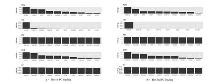
Figure 7. The selected stocks in the first two PCs for the periods after the outbreak. The stocks are arranged according to the absolute value of the loadings.

Table 4. The nonzero loading fields of of the first two sparse PCs (before the outbreak).

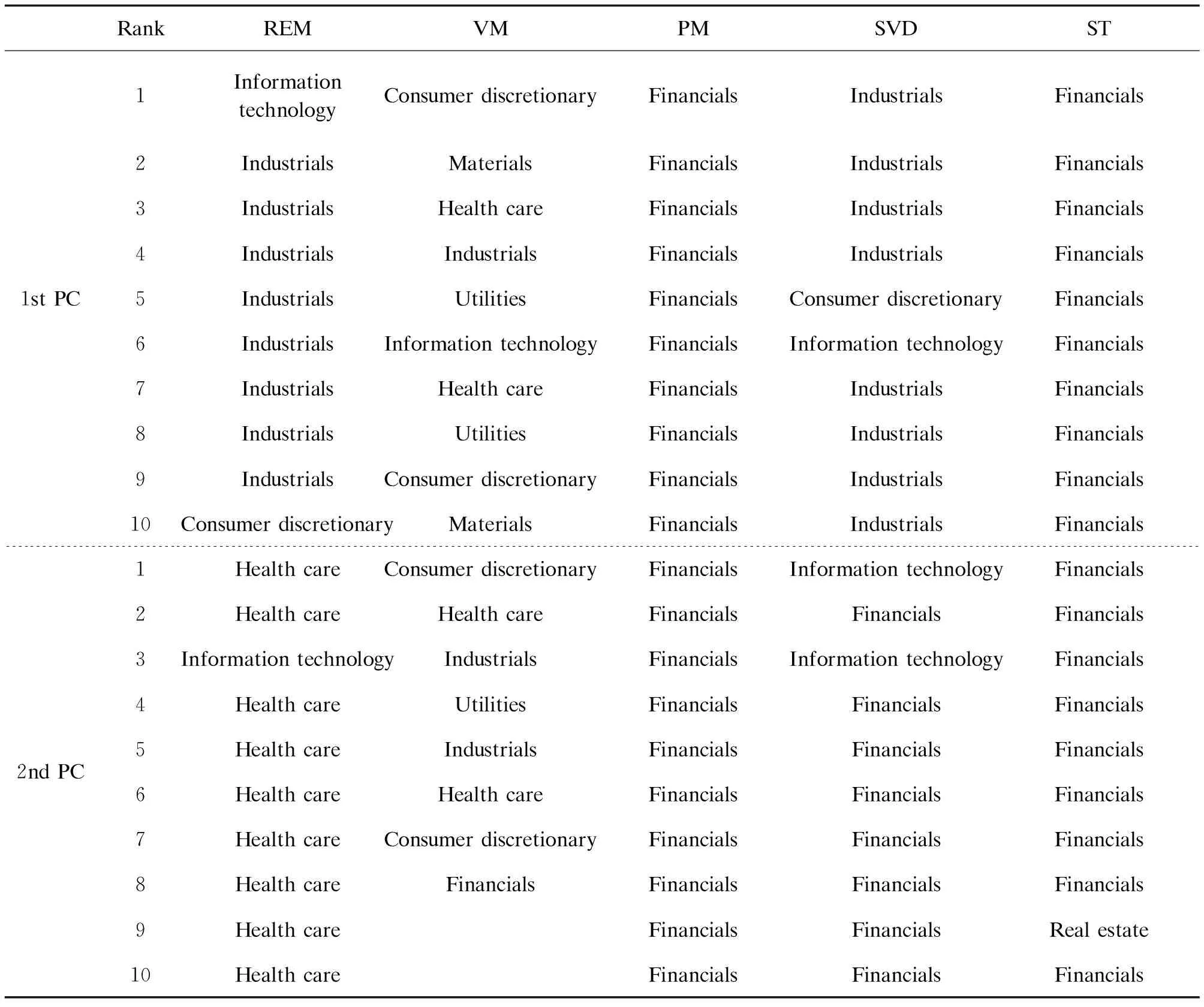
Table 5. The nonzero loading fields of the first two sparse PCs (after the outbreak).

In addition, according to the weights of sparse PCs, we can formulate a winning portfolio, which selects companies with nonzero loadings. As shown in Figure 8, the resulting portfolio will perform significantly better than the market because it invests in companies that have actually benefited from the pandemic. It can be seen that except for the PM and ST methods, all the other methods provide sparse PCs with better performance compared to the CSI 300 index. Regardless of whether it is formulated from the first or second PC, the return of PM and ST portfolio is lower than CSI 300 index. Based on the previous analysis, it may because that the stocks selected by PM and ST are mostly concentrated in bank stocks, which makes it difficult to diversify risks. The first PC of all methods has a similar trend to the CSI 300 index, which suggests that the first PC represents market risk. Compared with the first PC, the second PC of REM, VM and SVD portfolio are rising more steadily, surpassing most of the cumulative return of the first PC in the later period. In short, most of the sparse PCA methods yield better returns than the CSI 300 index, and the second PC has more robust and stable performance compare with the first PC. Combining the PCA results in Section 3.2, we can tell the reason that the cumulative returns of the second PC is higher than those of the first PC in the period after the outbreak. It is because the dominant stocks of the second PC are all from the health care and industrial fields, which have achieved rapid growth during the pandemic period.

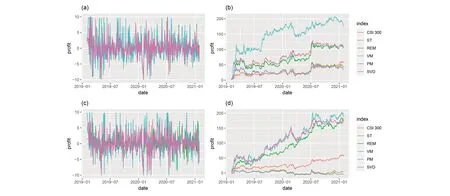
Figure 8. Portfolio for the stocks from the first two sparse PCs. The CSI 300 index is also included for comparison. The daily and cumulative portfolios are presented in the left and right panels, respectively.

Figure 9. Portfolio for the stocks from the first two sparse PCs. The CSI 300 index is also included for comparison. The 1st PC and 2nd PC are presented in the upper and down panels, respectively.

Finally, Figure 9 shows the return trend of the portfolio obtained from the sparse PC during the period of January 1, 2020 and April 20, 2020. We include the results of the REM and SVD methods as example. Compared with the classic PCA approach, the return trends show more volatility between the sparse PCA derived portfolio and the CSI 300 index. In specific, the portfolio of the first PC tends to have consistent performance with the CSI 300 index with a smaller variance, which is expected since it consists of stocks from the financial sector. The portfolio of the second PC have a total different trend, which can be explained by its composition, i.e., stocks are all from the health care and industrial fields.

4 Numerical research

In this section, we compare the performance of various algorithms on synthetic data. All programs are completed by R software, and the corresponding sparse principal component analysis methods are: ①VM, using R package: pcaPP; ②REM, using R package: elasticnet; ③M, using R package :Nsprcomp; ④SVD: Consider two algorithms: one is SVDb algorithm, the other is SVDc algorithm using R package: PMD.

4.1 Setting

In this section, we consider a more complex data generating mechanism by extending the studies in Hsu et al.[19]. Suppose we are given a sample covariance Σ coming from a “spiked” model of covariance, with

Σ=VVT+σ2Ip

where the columns ofV=(vij)∈p×3are the true sparse leading eigenvector,Ipis an identity matrix, andσ=0.1. A data matrixX∈n×pis then generated by drawingn=100 samples from a zero-mean normal distribution with covariance matrixΣ, that is,X～N(0,Σ).

Two dimension are considered:p=50 andp=100. In addition, we consider two different covariance structures:

① Non-overlap structure. (Figure 10(a))

② Overlap structure. (Figure 10(b))

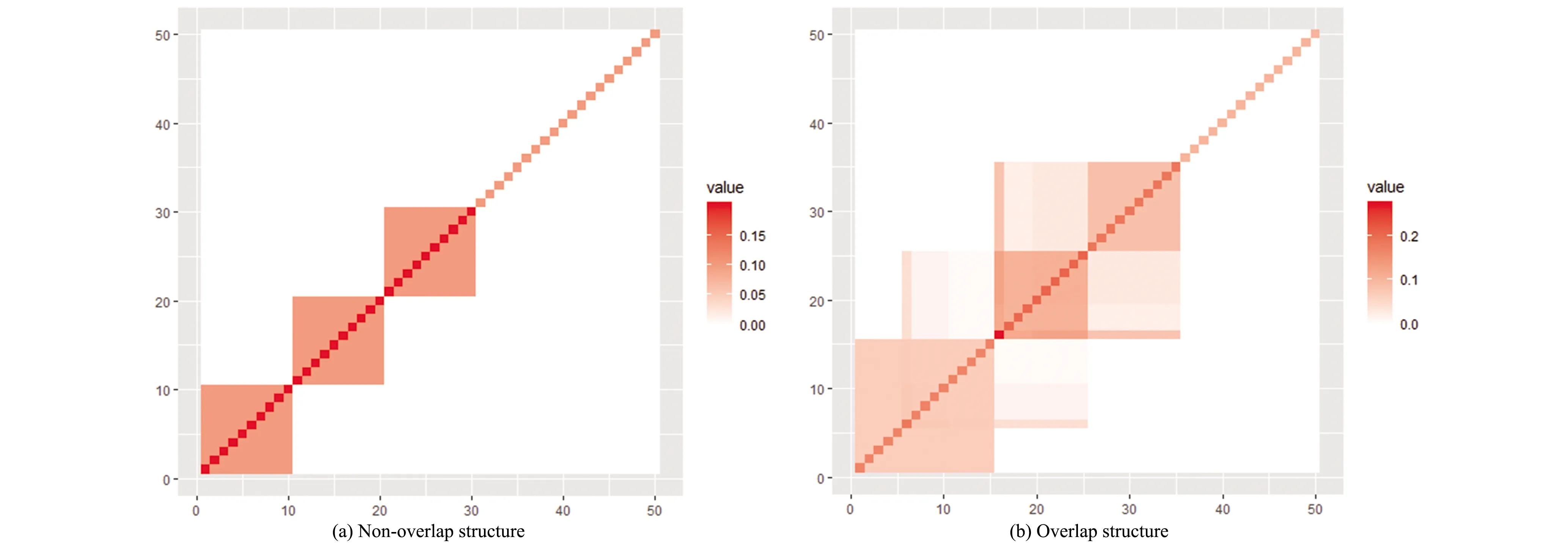
Figure 10. An illustration of the covariance structure in synthetic examples.

Therefore, four simulation scenarios are produced, they are: ①non-overlapping covariance structure, the number of variablesp=50; ②non-overlapping covariance structure, the number of variablesp=300; ③overlapping covariance structure, The number of variablesp=50; ④Overlapping covariance structure, the number of variablesp=300. The simulation in each case was repeated 300 times to estimate the first three principal components.

4.2 Results

Figure 11. Boxplots of the Consine values drawn by six algorithms: PCA, REM, VM, PM, SVDb and SVDc in four simulation schemes.

The results of the four simulation studies are plotted in Figure 11. Obviously, almost all sparse PCA methods perform better than classic PCA methods. This shows that the sparse PCA method can better estimate the load coefficient value. Comparing the non-overlapping covariance structure and the overlapping covariance structure, the sparse PCA method performs better in the case of non-overlapping covariance structure (Figure 11(a)-(b) versus 11(c)-(d)). In addition, for the sparse PCA method, it can be observed that the high coincidence rate of PC1 exceeds that of PC2 and PC3. Also, sparse PCA performs better when the number of variables is small (Figure 11(a) versus 11(b) or 11(c) versus 11(d)). From the four pictures in Figure 11, we can find that the REM algorithm, SVDb algorithm (R code written by Shen and Huang[11]) and SVDc algorithm (R software package PMD) perform well under any circumstances, while the VM algorithm and PM algorithm perform worse when the number of variables is greater than the number of samples (p>n). This shows that the REM and SVD methods are more suitable for high-dimensional small sample data. On the other hand, it shows that the stability of these two methods is stronger than the latter two algorithms.

5 Conclusions

The COVID-19 pandemic has caused serious public health and economic consequences throughout the world. It is very important to assess the impact of the pandemic on the economy, especially the stock market. It is of great interest to study the impact of the pandemic on the stock market via dimension reduction techniques such as PCA. In practice, it is important to figure out which stocks are inflected mostly by the pandemic and construct portfolio management based on them. To this end, we collected the CSI 300 stock data from February 1, 2019 to February 1, 2021, and divided them into two periods, i.e., before and after January 1, 2020, and applied PCA and sparse PCA methods to them. The results show that the outbreak of the pandemic led to changes in both proportion and constitution of the principal component of the stocks in the CSI 300 index. In addition, our research work compares four different sparse PCA procedures in CSI 300 data as well as simulated data, which would provide a practical guidance for financial applicants.

Studies have shown that the performance of each algorithm of principal component analysis varies greatly, and there still have room for improvement. In the future study, it is of interest to use other modern optimization algorithms (such as primal-dual active set algorithm[20]and mixed integer optimization algorithm[21]) to derive a more accurate estimation. In addition, our current work is based on historical data before and after the outbreak of the COVID-19 pandemic, which can be used as a dynamic tool for index selection in the future, so we need to think about ways to improve its generalization ability.