Least Squares Estimator for Fractional Brownian Bridges of the Second Kind

WANG Yihan(汪义汉)

(School of Mathematics and Statistics，Anhui Normal University，Wuhu 241000，China)

Abstract:In this paper，we study the least squares estimator for the drift of a fractional Brownian bridge of the second kind defined under the cases of parameter θ＞0 and Hurst parameter H∈We obtain the consistency and the asymptotic distribution of this estimator using the Malliavin calculus.

Key words:Fractional Brownian motion;Least squares estimator;Bridge

1.Introduction

LetT＞0 be fixed.For allθ＞0，the fractional bridge of the second kind{Xt}t∈[0，T)with initial value 0 is the solution of the stochastic differential equation(SDE)

In the case when the processXhas Hlder continuous paths of Hurst indexwe can consider the following least squares estimator(LSE)proposed in[8]，

as estimator ofθ，where the integral with respect toXis a Young integral.Thus，thanks to(1.1)，it is easily to obtain

In the same setup as fractional Brownian process of the first kind，the parameter estimation forθhas been studied by using classical maximum likelihood method or least squares technique by Barczy and Pap[4]，Tudor and Viens[13]，Es-Sebaiy and Nourdin[6]，HAN，SHEN and YAN[7]，respectively.In this paper，we consider the least squares estimatorin the setup of the fractional bridge of the second kind.The key point is the Lemma 3.6 in Section 3.

This paper is organized as follows.Section 2 deals with some preliminary results on stochastic integrals with respect to Malliavin derivative，Skorohod integral，Young integral.The consistency and the asymptotic distribution of the estimator are stated in Section 3.Almost all the proofs of the lemmas are provided in Section 4.

2.Preliminaries

We start by introducing the elements from stochastic analysis that we will need in the paper(see[1，11]).Letbe a fractional Brownian motion with the covariance function satisfying

The crucial ingredient is the canonical Hilbert spaceH(is also said to be reproducing kernel Hilbert space)associated to the Gaussian process which is defined as the closure of the linear spaceEgenerated by the indicator functions 1[0，t]，t∈[0，T]with respect to the scalar product

Therefore，the elements of the Hilbert spaceHmay not be functions but distributions of negative order.Let|H|be the set of measurable functionsφon[0，T]such that

It is not difficult to show that|H|is a Banach space with the norm‖φ‖|H|andEis dense in|H|.Forφ，ϖ∈|H|，we have

Notice that the above formula holds for any Gaussian process，i.e.，ifGis a centered Gaussian process with covarianceRinL1([0，T]2)，then(see[10])

ifφ，ϖare such thatdudv＜∞.

LetSbe the space of smooth and cylindrical random variables of the form

wheren≥1，f:Rn→R is a-function such thatfand all its derivatives have the most polynomial growth，andφi∈H.For a random variableFof the form above we define its Malliavin derivative as theH-valued random variable

By iteration，one can define themth derivativeDmF，which is an element ofL2(Ω;H⊗m)，for everym≥2.

For everyq≥1，letHqbe theqth Wiener chaos ofB，that is，the closed linear subspace ofL2(Ω)generated by the random variables{Hq(H(h))，h∈H，‖h‖H=1}，whereHqis theqth Hermite polynomial.The mappingIq(h⊙q)=Hq(B(h))provides a linear isometry between the symmetric tensor productH⊙q(equipped with the modified normandHq.Specifically，for allf，g∈H⊙qandq≥1，one has

On the other hand，it is well-known that any random variableZbelonging toL2(Ω)admits the following chaotic expansion:

where the series converges inL2(Ω)and the kernelsfq，belonging toH⊙q，are uniquely determined byZ.For a detail account on Malliavin calculus we refer to[11].

Letf，g:[0，T]R be Hlder continuous functions of orderμ∈(0，1)andν∈(0，1)respectively withμ+ν＞1.Young[14]proved that the Riemman-Stiltjes(so called Young integral)exists.Moreover，ifμ=ν∈(1/2，1)andΦ:R2R is a function of classC1，the integralsandexist in the Young sense and the following formula holds:

for 0≤t≤T.As a consequence，ifand(ut，t∈[0，T])is a process with the Holder paths of orderμ∈(1-H，1)，the integralis well defined as a Young integral.Suppose moreover that for anyt∈[0，T]，ut∈D1，2(|H|)，and

Then，by the same argument as in[1]，we have

In particular，whenφis a non-random Hlder continuous function of orderμ∈(1-H，1)，we obtain

Finally，we will use the following covariance of the increments of the noiseY(1)satisfying(see Proposition 3.5 in[9])

where

withCH=H2H－1(2H-1).Note that the kernelrHis symmetric.

3.Asymptotic Behavior of the Least Squares Estimator

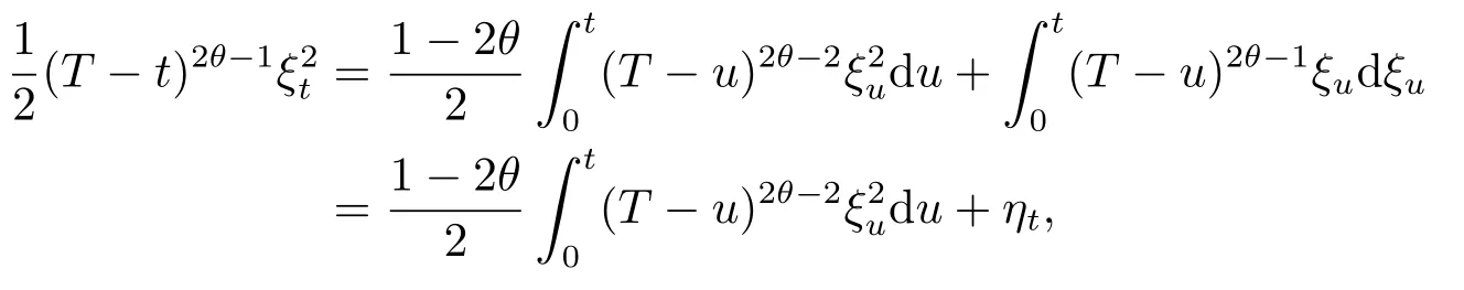
In this section we study the strong consistence and the asymptotic distribution of the estimator ofθtast→T.Consider the following processes related to{Xt}t∈[0，T):

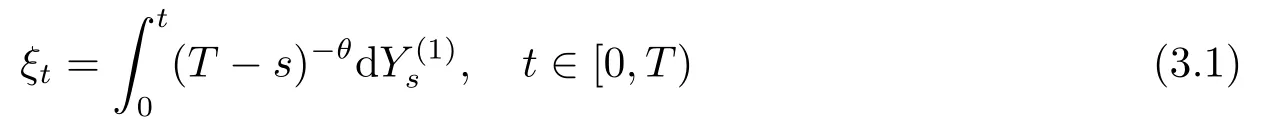
and

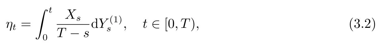
then，fort∈[0，T)and＜H＜1，

and

Using the equations(3.1)and(3.2)，the LSEdefined in(1.3)can be written as

ⅠConsistency of the Estimator LSE

The following theorem proves the(strong)consistency of the LSEFor simplicity，throughout this paper，letcstand for a positive constant depending only on the subscripts and its value may be different in different appearances，andstands for convergence in distribution(resp.probability，almost surely).

Theorem 3.1Letbe given by(1.3).Then

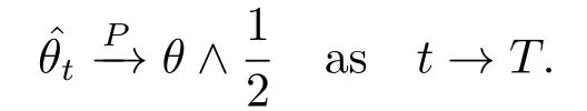
In particular，whenθ＜H，Hast→T.

In order to prove Theorem 3.1 we need the following two lemmas，and their proofs are shown in Section 4.

Lemma 3.1Supposeθ∈(0，H)，H∈and letξtbe given by(3.1).ThenξT:=limt→T ξtexists inL2.Furthermore，for allϵ∈(0，H-θ)there exists a modification of{ξt}t∈[0，T]with(H-θ-ϵ)-Hlder continuous paths，still denotedξin the sequel.In particular，ξt→ξTalmost surely ast→T.

Lemma 3.2Assumeθ∈(0，H)，H∈and letξtbe defined in(3.1).Then，ast→T:

1)if 0＜θ＜，then

2)ifθ=，then

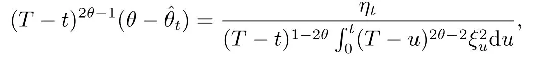
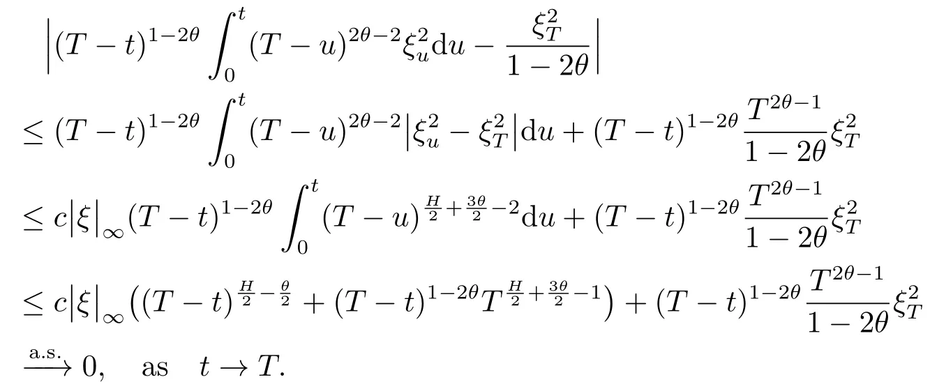
Proof of Theorem 3.1By the formula(2.6)，we obtain that，for anyt∈[0，T)，

which yields

Whenusing Lemma 3.2 and Lemma 3.1，we derive that

ast→T，respectively.Hence，we obtain thatast→T.

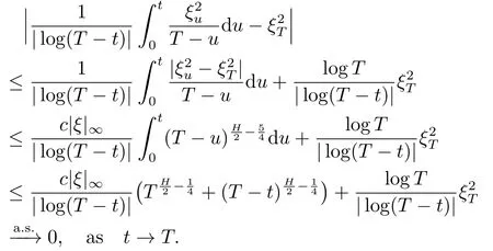
Whenθ=the equality(3.3)becomes

Analogously，by Lemma 3.2 and Lemma 3.1，we also deduce that

ast→T，respectively.Hence，we obtainast→T.

ast→T，respectively.Hence，(3.4)yields thatθ-ast→T，that is，

Finally，whenθ≥H，by(2.4)and(2.9)，and using the elementary inequality|ex-ey|α≤|x-y|αfor-1＜α＜0，x≥0，y≥0 andxy，we compute that

Hence，having a look at(3.3)and becauseast→T，we deduce thatast→T，that is，which implies the desired conclusion.

ⅡAsymptotic Distribution of the Estimator LSE

Theorem 3.2Assume＜H＜1 be fixed and setσ2=2H(2H-1)β(1-H，2H-1)withβ(a，b)=LetN～N(0，1)be independent ofY(1)，and letC(1)stand for the standard Cauchy distribution.

1)Ifθ∈(0，1-H)then，ast→T，

2)Ifθ=1-Hthen，ast→T，

3)Ifθ∈(1-H，)then，ast→T，

4)Ifθ=then，ast→T，

We also apply the following several lammas to prove Theorem 3.2，whose proofs refer to Section 4.

Lemma 3.3Letθ∈(1-H，H)，H∈and letηtbe defined in(3.2).ThenηT:=limt→T ηtexists inL2.Furthermore，there existsγ＞0 such that{ηt}t∈[0，T]admits a modification withγ-Hlder continuous paths，still denotedηin the sequel.In particular，ηt→ηTalmost surely ast→T.

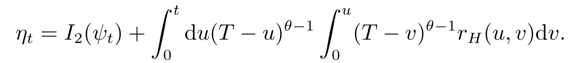
Lemma 3.4Letηtbe defined in(3.2).For anyt∈[0，T)，we have

Lemma 3.5Letθ∈(0，1-H]，H∈Then，ast→T，

Lemma 3.6Fix＜H＜1 and setσ1=σ2=2H(2H-1)β(1-H，2H-1).LetFbe anyσ{Y(1)}-measurable random variable satisfyingP(F＜∞)=1，and letN～N(0，1)be independent ofY(1).

1)Ifθ∈(0，1-H)then，ast→T，

2)Ifθ=1-Hthen，ast→T，

Proof of Theorem 3.21)Assume thatθ∈(0，1-H).By Lemma 3.4，we have

with clear definitions forat，bt，ct，etandft.Let us begin to consider the termsat，btandct.First，Lemma 3.6 yields

whereN～N(0，1)is independent ofY(1)，whereas Lemmas 3.1，3.2 imply thatandast→T，respectively.On the other hand，by combining Lemma 3.2 with Lemma 3.5，we can get thatandast→T，respectively.Let us summarize all these convergence together，we obtain that

2)Assume thatθ=1-H.By similar arguments as in the first point above，the counterpart of decomposition is the following:

By using Lemma 3.6 again，we obtain that，ast→T，

whereN～N(0，1)is independent ofY(1)，whereas Lemmas 3.1，3.2 also imply thatandast→T，respectively.On the other hand，by combining Lemma 3.2 with Lemma 3.5，we deduce thata ndast→T，respectively.By plugging all these convergence together we get that，ast→T，

3)Assume thatθ∈(1-H，).Using the decomposition

we immediately obtain that the third point of Theorem 3.2 follows from an obvious consequence of Lemmas 3.3，3.2.

4)Assume thatθ=By(3.4)，

4.Proofs of Several Lemmas

In this section，we present here the proofs of several lemmas used in Section 3.

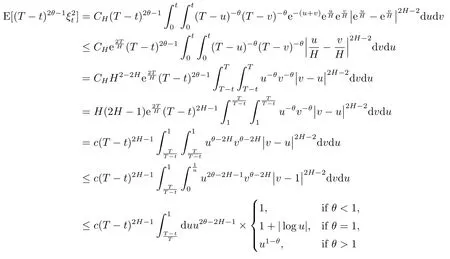
Proof of Lemma 3.1The idea mainly comes from Lemma 2.2 in[5]and Lemma 4 in[6].We give the main process as following for the completeness.In order to apply the Kolmogorov continuity criterium，we need to evaluate the mean square of the increment

with 0≤s≤t＜T.This is a Gaussian random variable and we will use the formula(2.4)in order to compute itsL2norm.The covariance of the processY(1)can be obtained from the formula(2.9).

Recall that the elementary inequality|ex-ey|α≤|x-y|αholds for-1＜α＜0，x≥0，y≥0 and.For all 0≤s≤t＜T，using(2.3)and(2.9)，we have

for some positive constantC(H，θ)depending onHandθ.By applying the Cauchy criterion，we deduce thatξT:=limt→T ξtexists inL2.Furthermore，because the processξis centered and Gaussian，for any positive integerm，we have

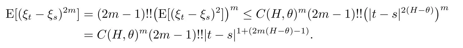
Hence，formsufficiently large satisfying 2m(H-θ)-1＞0，ξtareγ-Hder continuous for every=Therefore，the result follows directly from an application of the Kolmogorov continuity theorem.

Proof of Lemma 3.21)By Lemma 3.1，using the-Hlder continuity ofξt，we have

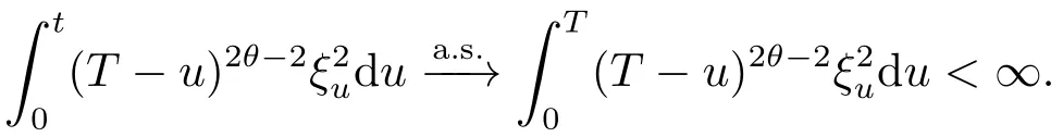
3)By Lemma 3.1，the processξis continuous on[0，T]，hence integrable.Furthermore，becauseu→(T-u)2θ－2is integrable atu=T.The convergence in point 3 holds with a finite limit.

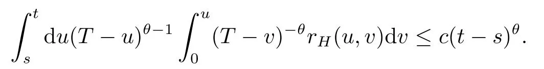
Proof of Lemma 3.3Letβ1，β2∈(1-H，H)be fixed.We first show that there existsε=ε(β1，β2，H)＞0 andc=c(β1，β2，H)＞0 such that，for all 0≤s≤t＜T，

In fact，by means of the change of variables，we have

≤c(t-s)εfor someε∈(0，1∧(2H-β1)-β2).

Therefore，the inequality(4.1)holds.

Now，using(2.7)，we shall separateηtinto two terms.Fort＜T，

Set

The identity(4.2)becomes

Therefore，by(2.5)，we have

Sinceψt-ψs∈H⊙2，we obtain that

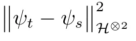
Notice the fact thatψt-ψsis symmetric，we easily get thatis upper bounded by a sum of integrals of the type

withβ1，β2，β3，β4∈{θ，1-θ}.Therefore，by(4.1)，there existsε＞0 small enough andc＞0 such that，for alls，t∈[0，T]，

On the other hand，for all 0≤s≤t＜T，we obtain again that

Thus，

Second，ifθ=2H-1 then

Thus，

Third，ifθ＜2H-1 then

Thus，

To summarize three cases above，there existsc＞0 such that，for alls，t∈[0，T]，

Substituting(4.4)and(4.5)into(4.3)yields that there existsε＞0 small enough andc＞0 such that，for alls，t∈[0，T]，

By using the Cauchy criterion again，we obtain thatηT:=limt→T ηtexists inL2.Furthermore，becauseηt-ηs-E[ηt]+E[ηs]belongs to the second Wiener chaos ofY(1)，the result follows directly from an application of the Kolmogorov continuity theorem.

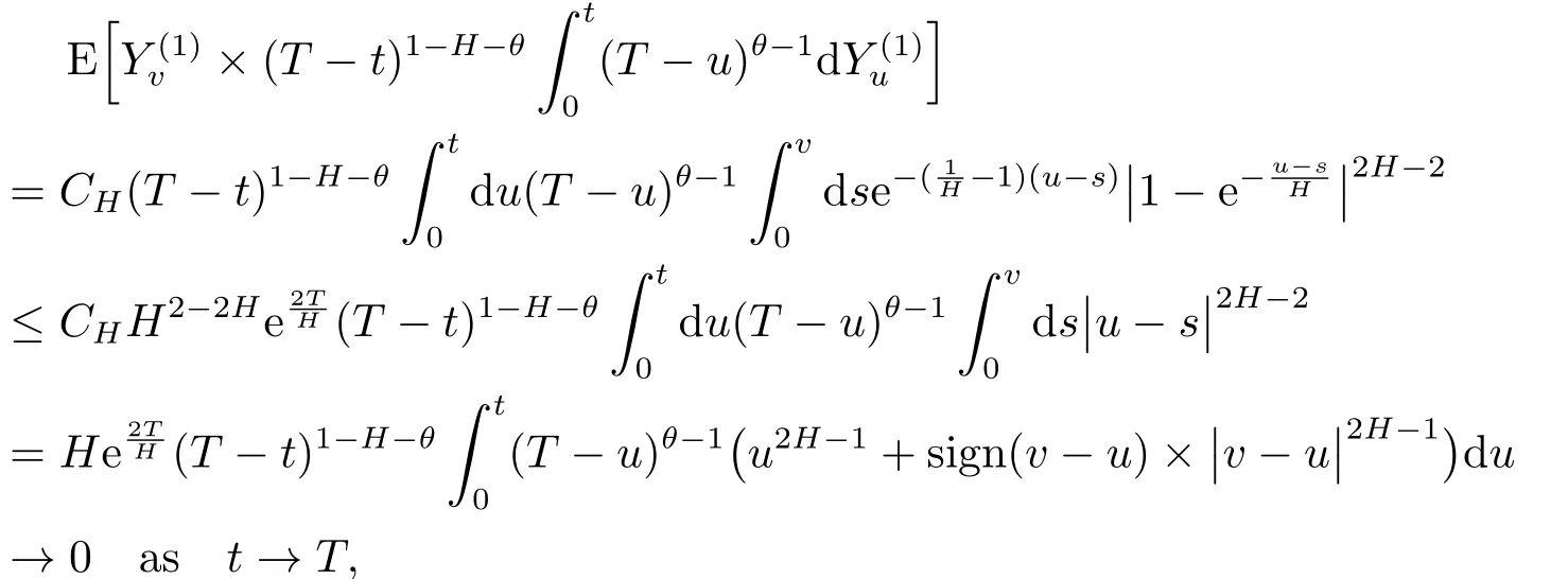
Proof of Lemma 3.4Lett∈[0，T)be fixed.By(2.6)，v)－θdY(1)vbecomes

Furthermore，it follows from(2.7)that

Hence，the result follows.

Proof of Lemma 3.5PutNotice thatφt∈|H|⊙2andwe obtain that

Sinceθ≤1-H，we obtain that

Furthermore，since 2H+2θ-3＜-1 andθ∈(0，1-H]，we obtain that

Hence，ifθ＜1-H，then

Assume now thatθ=1-H，then

Thus，by combining all the previous cases，we obtain that lim supt→Tis finite，which completes the proof.

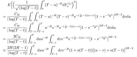
Proof of Lemma 3.61)We will use the approach from the proof of Lemma 7 in[6].It is enough to prove that for anym≥1 and anys1，...，sm∈[0，T)，we shall prove that，ast→T，

where，for|T-t|sufficiently small，

with

Thus，

On the other hand，by(2.9)we have，for anyv＜t＜T，

2)By(2.9)，for anyt∈[0∨(T-1)，T)and for|T-t|sufficiently small，we have

On the other hand，fixv∈[0，T)，by(2.9)，for allt∈[0∨(T-1)，T)，we have

whereσ2=2H(2H-1)β(1-H，2H-1).Therefore，the same reasoning as in point 1 allows to go from(4.7)to(3.6).The proof of the lemma is concluded.

AcknowledgmentsWe thank Professor Shen Guangjun for his guidance，including valuable suggestions and remarks and for his fund support.