PDE solution to UAV/UGV trajectory planning problem by spatio-temporal estimation during wildfires

Mohmmrez RADMANESH, Blji SHARMA, Mnish KUMAR,Donl FRENCH

a Aerial Mobility Group, NASA Jet Propulsion Lab (JPL), Pasadena 91016, USA

b Mathworks, Buffalo, New York, USA

c Department of Mechanical and Material Engineering, University of Cincinnati, Cincinnati 45221, USA

d Department of Mathematical Sciences, University of Cincinnati, Cincinnati 45221, USA

KEYWORDS State-estimation;Trajectory planning;UAV;UGV;Wild-fire

Abstract Unmanned Aerial Vehicles(UAVs)and Unmanned Ground Vehicles(UGVs)have been used in research and development community due to their strong potential in high-risk missions.One of the most important civilian implementations of UAV/UGV cooperative path planning is delivering medical or emergency supplies during disasters such as wildfires, the focus of this paper.However, wildfires themselves pose risk to the UAVs/UGVs and their paths should be planned to avert the risk as well as complete the mission. In this paper, wildfire growth is simulated using a coupled Partial Differential Equation(PDE)model,widely used in literature for modeling wildfires,in a grid environment with added process and measurement noise. Using principles of Proper Orthogonal Decomposition (POD), and with an appropriate choice of decomposition modes, a low-dimensional equivalent fire growth model is obtained for the deployment of the space-time Kalman Filtering (KF) paradigm for estimation of wildfires using simulated data. The KF paradigm is then used to estimate and predict the propagation of wildfire based on local data obtained from a camera mounted on the UAV. This information is then used to obtain a safe path for the UGV that needs to travel from an initial location to the final position while the UAV’s path is planned to gather information on wildfire. Path planning of both UAV and UGV is carried out using a PDE based method that allows incorporation of threats due to wildfire and other obstacles in the form of risk function. The results from numerical simulation are presented to validate the proposed estimation and path planning methods.

1. Introduction

Unmanned Air Vehicles (UAVs) have been used in military operations for a number of years.Recently,UAVs have generated increased interest due to their lowering cost and potential application in civilian domains such as emergency management, law enforcement, precision agriculture, package delivery, imaging/surveillance and providing Situational Awareness(SA).1SA is a broad term that refers to the comprehension of a set of event parameters of interest and their influence on the manner in which the event state evolves over a specific time horizon. The generation of real-time situational awareness for spatio-temporal processes such as wild-land fires, with the deployment of a multi-UAV system, presents a number of unique challenges in terms of fusion of data received from multiple distributed sources, often asynchronous,and additionally in terms of the computational complexity of processing large spatio-temporal data.2,3

Wildfire is the focus of this paper.In the past decade,the U.S Federal Government has spent 19.3 billion dollars to suppress wild-land fires which have destroyed 68.3 million acres of land.4,5Nine of the 25 fires that cost the federal government the most in U.S.history were described as forest, wild-land or wild-land/urban interface fires.6. The term Wild-land/Urban Interface(WUI)is typically used to describe areas where extensive vegetation mixes with numerous structures and their inhabitants. Around 32 percent of U.S. housing units and 10 of all land with housing are situated in the WUI regions,and WUI growth is expected to continue.7In windy regions,fire can be a threat to homes a mile or more away from the flame front making the neighboring regions prone to wildland fires.8Thus, wildfire can be the cause of economic and ecological losses and it poses a threat to people, property,and communities.9

This paper focuses on using a cooperative UAV/UGV system to perform critical tasks such as emergency supply delivery during wildfires. It should be noticed that, here, we define the cooperation as sharing the information from the UAV to the UGV for better path planning. Wildfires pose risk to the UAV and UGV, and their paths need to be planned so as to complete their mission as well as to be risk-averse.The UGV’s role is to reach a goal point,the UAV’s role is to provide information about wildfire to the UGV so that UGV can plan a risk-averse path. As such, there are three major components of the paper:(A)A computationally efficient solution for solving the wildfire model that predicts fire propagation based on initial information (that can be provided via satellites); (B) A computationally efficient correction method for predicting the fire propagation that uses a local and frequently updated information obtained by a UAV; and (C) a UAV/UGV cooperative path planning algorithm that uses the computationally efficient fire propagation method to plan its path which is safest and shortest.Here,we provide a background on current state of research on two aspects of this paper: (A) Fire propagation model; and (B) robotic path planning.

Modeling wild-land fires is a multi-scale multi-physics problem.Prior to this research,wild-land fires have been modeled based on data assimilation methods10,11and Dynamic Data-Driven Application System (DDDAS) techniques.12-14In the specific application of wild-land fires, the fire growth is typically modeled using a Partial Differential Equation(PDE) that can be solved using grid-based finite difference or finite element methods. Given the geographical spread of the environment over which such events occur and with the temporal aspect factored in, data from sensing systems for such processes are very high dimensional in nature, and thus developing a filtering mechanism that incorporates sensing data for online and real-time estimation and prediction for applications can be very challenging.The use of a multi-agent system in the sensing process adds to the complexity of the problem by introducing the additional challenge of sparseness, both spatially and temporally, in the data received.15

Path planning problem belongs to a class of Nondeterministic Polynomial-time (NP) hard problems which are usually solved for realistic problems by making some assumptions and using heuristics to reduce the complexity to that of the polynomial time problems.16The following studies covers the multitude of different motion planning algorithms for robots. In Refs.17-19, algorithms focus on polygonal obstacle field representations.Ref.20provides a survey of all the mathematical improvements in the field of motion planning.Ref.21considers the dynamic environment for robot path planning and provides information on computational bounds for limited cases. More recently,22,23studied sensor based path planning and probabilistic path planning methods. Ref.23emphasizes the implementation of these methods in ground vehicles.The following authors provide a comprehensive study of most of the available methods -24offers a review of all the applicable path-planning algorithms for different vehicles with an emphasis on ground vehicles,25presents the first comprehensive surveys carried out on heuristic methods. Surveys for UAV path planning have recently appeared in the literature and, among those,26provides a literature review for implementing path planning for autonomous vehicles.Ref.16specifically focuses on path planning of UAVs while27focuses on progress made in path planning and obstacle avoidance of Autonomous Underwater Vehicles (AUVs). There has been a lot of work carried out in the area of robot path planning on last few decades. Although the more commonly used path planning algorithms such as A*,Dynamic Programming, Gradient Algorithm, Newton Algorithm promise to find the most optimal solution,search space complexity due to large number of decision variables,which is more often what real world scenarios are all about, makes them extremely difficult to implement.28To address the issue of scalability, heuristic path planning algorithms such as artificial potential field, Genetic Algorithm (GA),29fuzzy logic,30Ant Colony Algorithm,31Particle Swarm Optimization (PSO)32and Grey Wolf Optimization (GWO)33have been used in literature.

Here, we introduce a PDE based method that combines mathematical rigor with scalability offered by the heuristic algorithms. PDEs are typically used to model system properties related to fluid mechanics and thermodynamics.They have also been proven useful in areas of modeling of mechanical and biological systems.34Partial resistance of fluid flow is among the first characteristics of the porous media to be considered.For example,fluid flows from a source to a sink point due to the sink point’s lower potential energy.During this process, the fluid finds the path with the highest permeability zones or the path of least resistance. The same behavior can be found in heat transport where the material’s thermal conductivity dictate the path that heat travels. This paper utilizes the fluid mechanical property of flow in porous media for the purpose of trajectory planning of UAV and UGV. The paths followed by the UAV and UGV correspond to the fluid streamlines that go from initial to final locations avoiding non-porous regions. In what follows, we first describe the problem addressed in this paper, and the contributions made by this paper.

1.1. Problem description

The problem considered in this paper is inspired from a search and rescue mission. In case of wild-fire, in vast areas, emergency supplies are considered to be delivered by trucks or as suggested in this paper, a UGV. The scenario starts with a given map of the environment. The UAV initiates its mission to scoop over the region for gathering the data on fire location.That information is used to predict the propagation of wildfire which is then used to help the UGV in planning of its path.Updates to the path are done in real time. The scheme of the mission can be explained in these steps:

· The initial map of the environment with hot-spot location is received from satellites.

· The above map is then used to predict fire propagation using the proposed spatio-temporal Kalman filter based on available information about topography and vegetation.

· Based on the fire propagation prediction, the trajectory for both UAV and UGV are obtained using the proposed PDE method35,36of trajectory planning.

· UGV and UAV start their missi（o n from） the depot(x0，y0，z0) to reach the goal position xf，yf，zf.

· UAV updates the fire-map based on partial data that it gathers and uses that to update the prediction using the proposed Kalman filter approach.

· Trajectory for the UGV is updated based on the current fire map

1.2. Contributions

The main contributions of this paper are to(A) develop a fast and efficient estimation process for event states evolving in space and time towards improved SA,and(B)propose a novel physics-inspired UAV/UGV trajectory planning that allows consideration of path-risk in obtaining optimal trajectories.This paper proposes a filtering method within the Bayesian framework harnessing concepts in Proper Orthogonal Decomposition (POD) for dimensional reduction. The rationale behind the proposed approach is that methods such as POD facilitate reduced-order modeling, thus reducing the computational complexity. Implemented in a grid-based model of the environment, the approach can eventually be integrated into Geographic Information Systems(GIS)for effective utilization of information and decision making for incident managers.

Fire growth is simulated using a coupled PDE model in a grid environment with added process and measurement noise.This simulated fire is used as ground truth data in all the numerical simulations presented in this paper. Using principles of POD,and with an appropriate choice of decomposition modes,a low-dimensional equivalent fire growth model is obtained for the deployment of the space-time Kalman filtering paradigm over the simulated data.The proposed space-time Kalman Filter based method of predicting the wild fire is used to obtain a risk function which is then utilized to derive collaborative UAV/UGV trajectory planning method. The trajectory planning method is inspired by use of PDEs in fluid mechanics,thermodynamics, circuits, and heat transfer. PDEs are used to model the fluid flow throughout the domain through the derivation of the surface’s porosity. The non-porous part in the fluid domain is considered to be analogous to threats in the environment where UAVs cannot pass through. The composite risk function used in this method considers threats that include fixed obstacles, detected threats, exclusion zones, fuel limits, required waypoints, UAV dynamics, and time constraints. Extensive flight path simulations were performed and the results confirmed the robustness of the proposed solution in large and complex domains/environments36.

Although this paper provides a use-case scenario for the trajectory planning in the area of wildfire, it should be noted that the proposed method can be extended to trajectory tracking of robots under any other scenario where risks could be modeled as spatio-temporal processes that capture the dynamic nature of the threat. Such spatio-temporal processes,represented by PDEs (similar to wildfire propagation model),for example, have been used in literature to model criminal or terrorist activities37. The rest of the paper is organized as follows.In Section 3,a mathematical model of wild-fire growth is presented.Here,first a popular PDE model used in literature for fire-propagation is presented. It may be noted that this model is used in this paper for simulating the ground truth wildfire data. Subsequently, a Kalman Filter (KF) based space-time filter based on the PDE model is proposed that provides a computationally efficient way of predicting the fire based on online sensor information. First, the Proper Orthogonal Decomposition(POD)technique that is used by the KF is explained, and then the KF based method is presented. Section 4 presents the path planning problem and the associated PDE/mathematical model in detail. A control solution using Cahn-Allen shape equation is proposed. Subsequently, risk evaluation and path post-processing are discussed this section.Finally, in Section 5, results and discussions are presented.

2. Fire growth model

This section presents a popular fire growth model based on coupled Partial Differential Equations (PDEs). This model is used in this paper for generating ground truth data of fire evolution over space and time. Subsequently, the underlying dynamics of the fire model is used in the Kalman Filter based computationally efficient method that is used to predict the fire growth. The fire growth can be represented by the set of coupled PDEs given by Eq.15:

The supply consumption rate is described by:

with the initial values s(t0)=1 and T(t0)=T0.

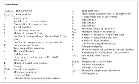
T(Λ，t ) and s(Λ，t ) represent, respectively, the temperature of the fire layer and the fuel supply mass fraction (relative amount of fuel remaining -s ∈[0，1 ]). The term Λ represents the vector of spatial variables, and t represents the temporal attribute.

Tarepresents the ambient temperature, and k represents thermal diffusivity. A is the rate of temperature rise at the maximum burning rate with full initial fuel load and in the absence of cooling. B and C1 are coefficients corresponding to the modified Arrhenius law and the heat transfer to the environment respectively. The fuel disappearance rate is given by Cs. The wind speed is represented by ν.

2.1. Proper Orthogonal Decomposition (POD)

The POD method relies on decoupling the spatial and temporal components of the event state to allow for a linear approximation to be constructed in a form represented by Eq.(3).38,39.

For mathematical convenience, Λ is stacked into a onedimensional spatial vector. ai(t ) represents time dependent amplitudes, referred to as time coefficients, and Ψi(Λ ) are spatial basis functions, also referred to in some works as trial functions. The method relies on the determination of the functions Ψi(Λ ) that have the largest amplitude ai(t )= ＜u(Λ，t )，Ψi(Λ )＞ in a mean-square sense, with＜...，...＞representing the inner product on Λ.

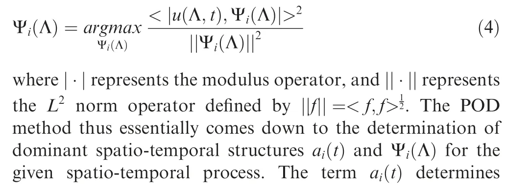
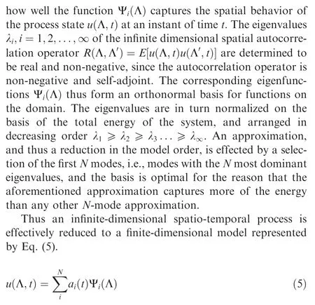
The spatial domain is typically discretized into a grid, and can very often lead to a very large spatial autocorrelation matrix. Solving the eigenvalue problem for such highdimensional data can be computationally very intensive. To circumvent this, the autocorrelation matrix for the eigenvalue problem can be constructed using what is referred to as the Method of Snapshots.Consider M snapshots of the event state u(Λ，t ) taken at regularly spaced intervals Δt with each snapshot defined by ui(Λ )=u(Λ，iΔt). The autocorrelation matrix is then approximated by Eq. (6) and facilitates, subsequently,the POD process with reduced dimensionality.

The spatial basis functions can then be computed as the linear combinations of the data snapshots using Eq. (7).

where Akrepresents the eigenvectors corresponding to the eigenvalues λkobtained from the solution of the eigenvalue problem discussed hitherto.

The matrix of time coefficients, A, can be computed as the solution of Eq. (8).

where S represents the m×m snanpshot matrix and Φ represents the matrix of spatial basis functions computed using Eq. (7), i.e., Φ= [Ψ1，Ψ2，...，Ψm].

Further,a selection of the first N dominant modes(N ＜m),with the maximum variance between them,allows for approximating the process with a reduced dimensional model. An optimal choice of N would in turn yield a fairly accurate, yet lower dimensional, equivalence without significant error. The matrices for the spatial basis functions, Φ, and time coefficients, A are consequently truncated to retain only those corresponding to the first N modes used for reconstruction of the process.

2.2. Space-time Kalman filter based estimation

Assuming the process and measurement models satisfy linear and Gaussian assumptions, a space-time Kalman filter can be implemented in a manner described ahead. The temporal dynamics of the time coefficients are modeled using a firstorder multivariate autoregressive model (AR1) represented by Eq. (9).

The terms H and Jηare obtained as parameters of the multivariate AR1 model, and form the basis for the process equations. The space-time Kalman filter, in conjunction with the decoupled spatial basis functions and time coefficients, is described in Eqs. (10)-(14).

The prediction equations for the state and covariance matrices are given by:

where j is the spatial error covariance matrix, and J= (Φ′Φ)-1Φ′, with Φ representing the matrix of spatial basis functions for the truncated set of modes, N.

The Kalman gain ι (t ) is computed as in Eq. (12).

The measurement updates for the state and error covariance matrices are presented ahead in Eqs. (13) and (14)respectively.

Once the filtered time-coefficients are obtained through the estimation process, the estimated process is determined by resynthesizing the decomposed model using Eq. (15).

2.3.Solution control by Cahn-Allen equation in spatio-temporal environment

The main aim of this section,is to provide a correction method for the estimation, provided in Section 2, which was resulted from the entry data to our fire propagation POD method.The motivation behind this correction is that, while the UAV is flying over the fire region, it can provide an actual observation for a state and fire status in the specific statespace. Upon having a disturbance in the region, such as a non-vegetation area, in the middle of vegetation region, the estimation requires corrections. The numerical method of corrections for this estimation method is provided in this section.

The finite difference method introduced in previous section is a numerical technique used to solve differential equations by partitioning the domain to be approximated into a finite space and then assembling simple elements to fill in the finite space.The main idea is to consider the current condition at time trto correspond to the prediction in function H(t，Λ )=∑

Λu(t，Λ ),where s in Eqs. (16) and (17) represents the numeration for Cahn-Allen method.Then H can be used as a history for each cell from the initial condition to the current condition,and ^u is the solution obtained from Eq. (15). Furthermore, in this problem, Λ ∈[x，y ]. Inspired by Cahn-Allen energy equation for reformation of PDE problems,40, we consider:

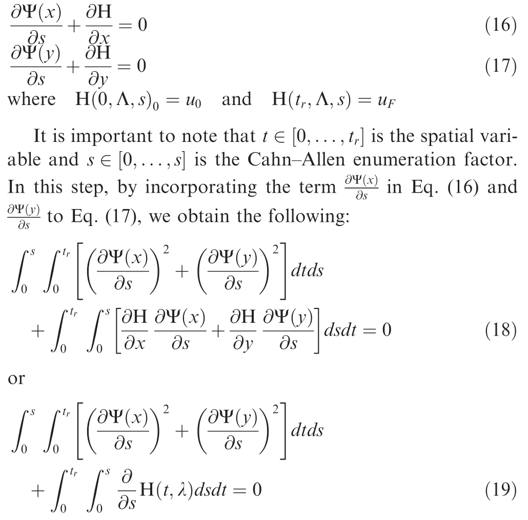
Approximation of Eq. (19) gives:

Since the right hand side of Eq. (20) is decreasing until the changes with respect to s for X and Y stop, we expect the left side to decrease and tend to a minimum.This control over the solution benefits the system for accuracy over the solution updates received from UAVs. In essence, H(Λ，t，0) is the first guess to this problem.If the second integral on the right handside of Eq. (20) tends to zero, then the function H(Λ，t，s) is a good guess for the update of the rest of the grids.By indication of the right hand side of equation and solving this for the uniform grids,the gradient of Ψ(Λ )can be generated and the estimation can be reformed from this step.

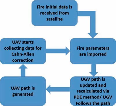
Fig. 1 Process of UAV/UGV path planning.

This method is used as feedback to correct the estimation generated via Kalman filter with consideration of time. The estimation is imported in the proposed algorithm in the scheme shown in Fig. 1.

2.4. Risk evaluation

The risk function is analogous to terms representing permeability in Eq. (27) in an opposite fashion. The risk functionhas low values in the areas of low risk. Since low risk areas are more favorable,the permeability values are higher in those areas. The fluid moves more freely through the cells with higher permeability values. Eq. (21) modifies the permeability as follows:

The function κ transforms the risk values of functioninto the permeability function.In this evaluated problem,the function κ is considered as:

The variable αis considered constant and β ∈R+. Physical values of κ are used to generate the optimal trajectory. If the risk value is very small it may be neglected from the analysis.Hence, in this work, the LΥis considered as the minimum risk and this value is neglected while the risk is not high.

LΥ∈R+represents a small constant and are considered in this paper to be small value near 0.

3. Path planning problem

3.1. Cost function

The path with minimal accumulated risk is determined through optimization of a cost function that integrates the risk function throughout the path. It may be noted that multiple solution paths may exist due to the nature of PDE solutions.For a path R in the 3-Dimensional domain Υ，FR, the total accumulated risk value can be found via Eq.(24),whererepresents the risk function.

The optimized path, R*is found through solving the optimization problem formulated as:

The two simple UAV/UGV constraints considered in this function are maximum path length (Lmax) and largest achievable path curve (ψmax). The term t is assigned to show that the path R is a continuously differentiable function to the degree t. Other constraints can be added to Eq. (25) to form the optimization problem.The risk(x，y，z)is evaluated using a discrete representation of the risk function for Υ where Υ is the constrained three dimensional domain.

3.2. Partial Differential Equations

The Continuity Equation of fluid mechanics is used as the basis function f for generating all of the possible path solutions in the porous domain Υ. This is represented in Eq. (26) where φ is the porosity of the evaluated three dimensional point, ρ is the density of the fluid, and u is the velocity of the fluid.

Darcy’s Law is applied to (27) to describe the flow of the fluid through the porous domain. The steady state solution of (26) can be presented as:

where κ is the permeability of porous medium.

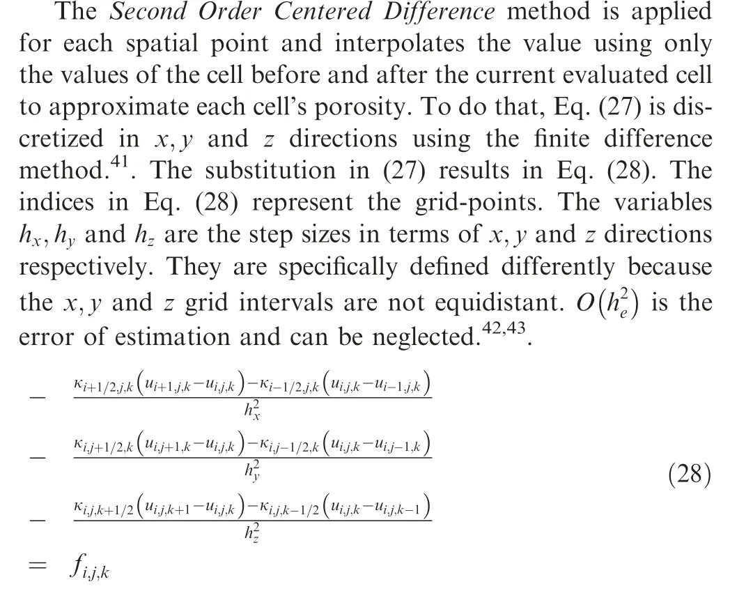
The variables (i，j，k) in Eq. (28) represent the cell labels of the tessellated area. The PDE Eq. (28) is solved for the entire domain Υ constrained by the boundary conditions.

3.2.1. Post processing of PDE

The results of Eq. (28) are multiple streamlines exposed to the gradient of u at every grid point. Since there is only one starting point and one final point in the domain, the number of solutions are reduced by applying the flux boundary conditional constraints which requ（ ire that） solutions start at t0at(x0，y0，z0) and finish at tfat xf，yf，zf.

In the domain Υ, multiple streamlines or flow paths from the origin to the goal position are generated. Incompressible flow dynamics represented by Eq.(28)dictates that the streamlines follow the velocity fields and finish at the goal position.The streamlines are evaluated with the optimization Eq. (25)and are converted to arrays of (x，y，z) points using the Runge-Kutta Method (RKM). Explicit one-step timestepping schemes of Eq. (25) can be expressed as:

It is noted that m is the number of functional evaluations and is also called the number of Runge-Kutta stages. In this paper, we are using the second order accurate scheme, developed by Cabuk et al.44

Eq. (29) returns all the routes that travel from the initial point to the goal position and have acceptable risk values. In other words,from Algorithm 1,we obtain components in each direction (i.e., for x and y and directions for 2D cases using a central difference method), such that there is no conflict with no-porous domain.By solving the equations of motion in porous medium(i.e.,Eq.(28))and finding all the possible streamlines which do not cross the obstacles, we have reduced the solution space to a manageable size.Considering that the risks represent the solid(non-porous part)space in porous medium,the solution streamlines represented by parameters k1，k2，...do not cross the areas with high risk values. Dynamical and kinematic constraints of the robots are then applied to the rest of the post processing.

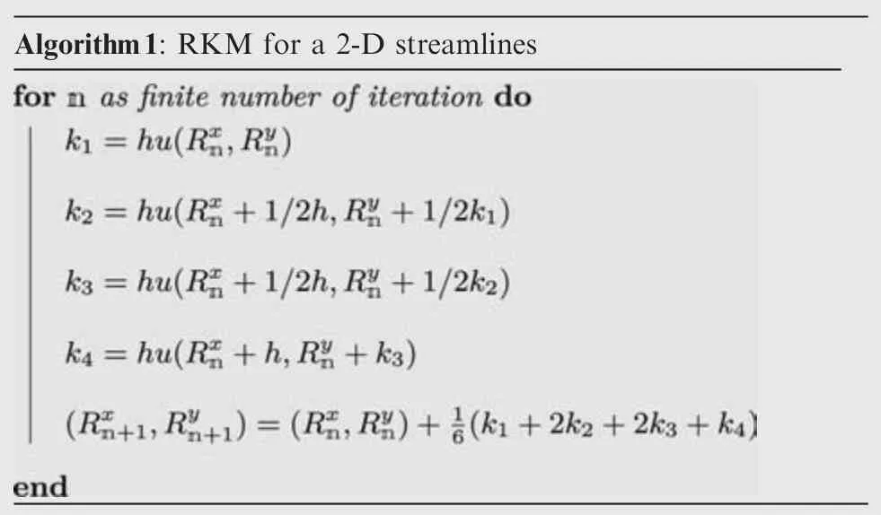
Algorithm1: RKM for a 2-D streamlinesimages/BZ_613_1282_1968_2109_2428.png

3.2.2. Minimal risk constraint

The cost function, defined in Eq. (24), is evaluated in the discrete domain during the computation of every path R. Eq.(31) produces the accumulated risk for path R.

Variable v represents the cells in path R.The RKM process restricts path length and eliminates undesirable paths.

3.2.3. Constraints on trajectory length

Undesirable trajectories are eliminated using the constraints described in Eq. (32). This eliminates several paths that are results of the path generation process.

It is noteworthy that Lminand Lmaxcould be defined for the type of UAV/UGV and the average fuel consumption for the vehicle.

3.2.4. Boundary conditions of PDE

Shown in Eq.(33),zero flux boundaries,also known as homogeneous Neumann boundary conditions, are used in problems with domains of extensive size.

The variable n is the unit vector along x，y or z direction.These conditions force the generated streamlines to become parallel to the boundaries of domain Υ when they become sufficiently close to them eliminating chances of paths going out of the domain.

After adding the boundary conditions to Eq.(34),the PDE can be represented as:

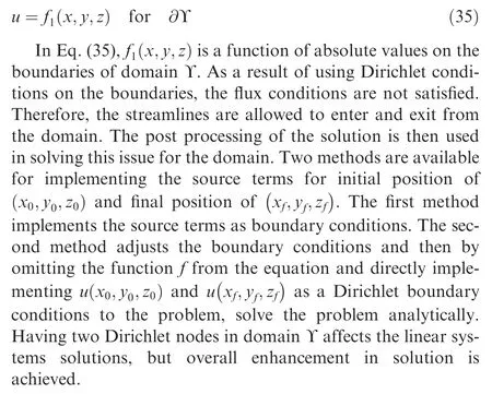
The Homogeneous Neumann conditions implemented on the whole boundaries of domain cause fluctuating streamlines near the boundaries as a solution for linear system of equations. Dirichlet boundary conditions shown by Eq. (35) can solve this issue.

3.2.5. Computational domain Υ and error evaluation

The computational domain is a tessellated area of uniform grids in the x-y plane and varying size in z directions. The aim is to calculate the near optimal trajectory in the uniform grids. However, another possible method for discritizing the domain uses an unstructured grid and solving with Finite Element Methods (FEM) but, these methods, may generate many erroneous results and are computationally expensive45.

Theorem 1. If a topographical function, defining the surface on which the fluid flows,is considered a flat surface in the indicated domain Υ,the error of the numerical solution of path planning is negligible.

Proof for Theorem 1 is provided in Appendix A.

Based on Theorem 1, for non-flat topographical maps, a solution is presented as follows:

-Tessellation of an area must be done in a way to generate group of cells with flat and smooth surface.

- For solution, the undesired cells which cause a nonsmooth topographical map must be removed.

- A combination of unstructured cells near surface and structured cells above surface should be maintained.

The proposed method is a desirable approach as it has shown to provide acceptable solutions that require less computational time.The method was applied to realistic flight scenarios and it was shown that the proposed method has a better performance than some of the other popular methods in literature in terms of optimality and computational time.35

3.3. Fixed obstacles and waypoints to visit

The presence of a fixed obstacle in the risk functions must be represented by an extremely high value. In this case an array O(x，y，z) which represents the obstacles, is defined as show in Eq. (36).

where UΥis a large positive number representing an upper bound of risk value.The UAV/UGV has predefined waypoints to visit during its mission. There are intermediate waypoints set for the UAV/UGV to visit during its mission before reaching the goal position.The priority of the waypoints are defined a priori. The waypoints are handled by successively setting each waypoint as the goal location and the analysis is repeated iteratively for each consecutive waypoint.

3.4. Cost evaluation

The scenario for fire temperature is different from that of the fixed obstacles. These areas with higher temperature is predicted by Section 2. Then, a higher risk value needs to be assigned for the cells within areas which have higher predicted temperature.In this paper,the value of the risk associated with the cells in these areas has been set to uΥand is shown by Eq.(37).

By combining the result of permeability and the temperature profile, the cost function is reformed based on the accumulation of temperature and fixed obstacle cost.

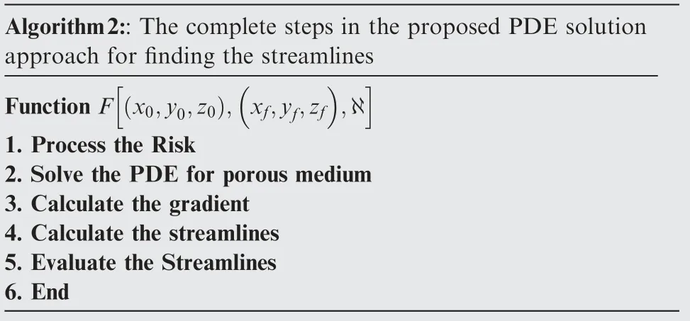
The total PDE solution for finding the streamlines can be summarized in Algorithm 2.

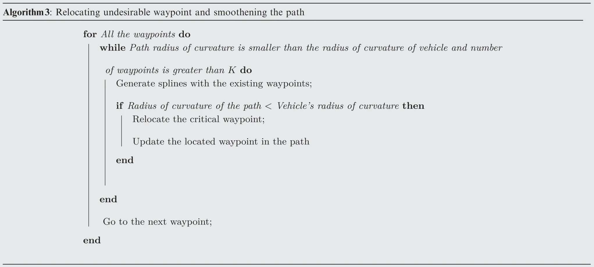
3.5. Post processing of path

A thorough comparison of the proposed method with other methods are provided in Ref.35It is shown that this technique provides more efficiency and better performance for highly complex trajectory planning problems in dynamic environments.

4. Results and discussion

?

In this paper,it was tried to direct the UGV to goal position in wildfire land to deliver supplies and goods. The process starts with the fire growth and the estimation process. Then this fire will propagate and the estimation is kicked into predict how the fire would react. Next step is to launch the UAV and UGV and perform the proposed path planning solution. During the results and discussions,multiple scenarios were studied to provide the performance of the solution.

It is assumed that the vehicles presented here,have a simple kinematic model as:

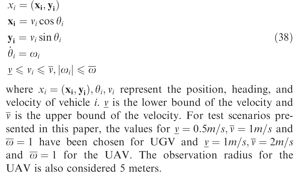
For this study, the fire growth data is generated using the model described in Eqs. (1) and (39) and is corrected via Eq.(20). The parameters for the fire growth model are listed below,considered from the fire growth model parameters presented in Ref.47The influence of ambient wind conditions is considered negligible.

Algorithm3: Relocating undesirable waypoint and smoothening the path?

k=0.2136 m2/sk3

A=187.93 k/s

B=558.49 k

C1=4.8372e(-5 ) 1/k

Cs=0.1625 1/s

T0=Ta=300 K

4.1. Estimation process

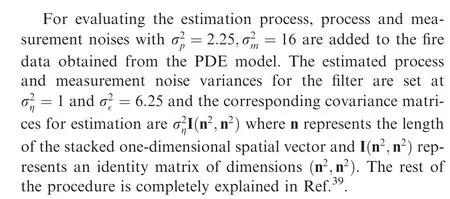
The initial conditions of the fire are represented in Fig. 2. For fire propagation,we use two methods:(A)Use finite-difference solution for PDE model presented in Section 3 obtained over a spatial grid of dimensions 415×415 units, and for a temporal length of 400 time-steps with a resolution of 1 unit. This represents, in this paper, ground truth fire data (i.e., how the fire propagates actually).;and(B)Use the proposed Kalman-Filter and POD based method for prediction based on information obtained from the UAV. This represents the predicted data.

In Fig.2,black circles and grey circles represent the hottest and nearby spots in the area. These are the places that the UAV and UGV need to avoid,while traveling within the area.

4.1.1. Scenario 1: Static condition/without any prediction

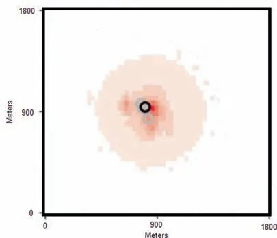
Fig. 2 Initial conditions for wild-fire.

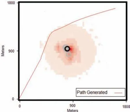
Fig. 3 Scenario 1: Initial path generated for the UGV without any prediction for wild-fire (considering current conditions).

The initial map of the area with fire, and the path which was generated ‘‘without” considering any prediction of fire at time t0is shown in Fig.3.Here,we assume static condition,i.e.,fire does not propagate. The UGV decides its path based on current condition. Here, to demonstrate the effectiveness of the PDE trajectory planning technique, the UGV trajectory planning cost with static fire, provided in Scenario 1, is compared with the potential field path planning algorithm48. The path length for the PDE technique (i.e. Fig. 3) was better than the cost provided in potential field function (path length for PDE technique is 2124 meters and path length for potential field path planning algorithm is 2523 meters).

4.1.2. Scenario 2: Estimation without uncertainty

In this scenario,the fire is assumed to grow but with conditions fully known.Under these conditions,the predictions based on the POD-Kalman Filter based method would be very similar to that of the actual fire growth. The estimation process is implemented as discussed previously, and the results are presented ahead. All computations are performed in the MATLAB R2016b environment on a 64-bit Windows-based PC with a dual core processor with a clock speed of 3.10 GHz and 8 GB of RAM. The estimated propagation of fire using the POD-Kalman Filter model is shown in Fig. 4.The actual path for the UGV obtained using the proposed PDE based path planning method using this predicted information at the end of t=400 time steps is shown in Fig. 5.

4.1.3. UAV waypoint generator

4.2. Path planning uncertain and unknown conditions

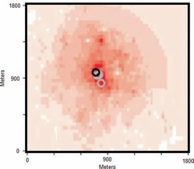
Fig. 4 Scenario 2: Estimation of wild-fire at t=400 time steps.

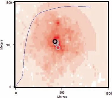
Fig. 5 Scenario 2: Path calculated for UGV by considering the risk function of wild-fire in t=400) time steps; path length is 2561.3 meters.

In this case, it is assumed that the Kalman filter provides the estimation of fire in presence of geographic and environmental effects such as change in wind direction or fuel supply (which in Scenario 2 were kept constant).These effects are not known a-priori. Here, the propagation of fire is expected to change(with respect to simulations with constant values assumed earlier) at each time step. As such,

4.2.1. Scenario 3: Environment with less uncertainty

In this experiment, the UAV starts to fly around the environment and collects the data from its sensor footprint.The actual propagation of wild fire for time steps t=220 and t=400 is shown in Fig.6.The UAV continues to fly in the environment following the pre-defined waypoints and collects the information. The partial information thus collected is fed to the Kalman Filter which predicts the fire propagation. That information is used to update the risk function in an online fashion which is then used to drive the UGV towards the goal position.

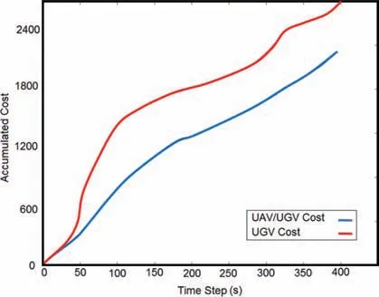
Fig. 7 Scenario 3: The accumulated cost function for the two cases: i) UGV only (no updates from UAV) and ii) UAV/UGV collaborative scenario.

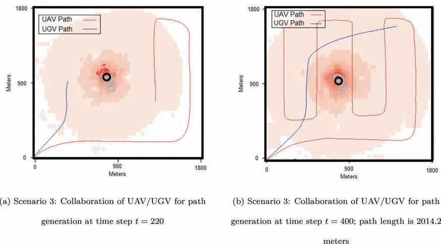
Fig. 6 Scenario 3: Environment with less uncertainty.

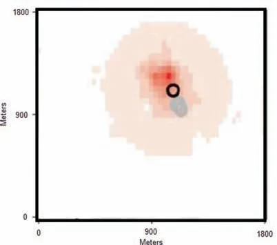
Fig. 8 Scenario 4: Initial conditions for wild-fire in second scenario.

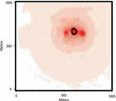
Fig. 9 Scenario 4: Estimation of wild-fire at t=400 time steps.

The accumulated cost (risk) function for two cases are shown in Fig. 7: (A) where UGV acts alone based on initial information obtained from the satellite; and (B) where UGV acts based on updated information obtained from the UAV.As can be seen, the total cost function is also reduced from 2561.3 to 2014.2 at the 400th time step.Furthermore,the path length of the UAV, is improved by 20% which indicates the importance and the effect of the proposed method.

4.2.2. Scenario 4: Environment with high uncertainty

In this scenario, wind is assumed to blow with the magnitude of 30m/s in the -x direction, starting from time step 0. It causes the wild-fire to propagate faster than the earlier scenario. Figs. 8 and 9 represent the initial hot spots and the fire propagation estimation, using space-time Kalman filter,resulting from constant condition at t=400 time steps respectively.

Fig.10 represents the two method of trajectory planning for the second scenario. It is noteworthy that in UGV method(without updates from UAV), the UGV is passing through the fire at t=343 time step. This result represents the significance of the UAV/UGV collaborative trajectory planning.

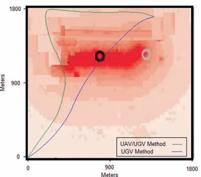
Fig. 10 Scenario 4: Trajectory of UGV in second scenario for the two cases:i)UGV only(no updates from UAV)and ii)UAV/UGV collaborative scenario at t=400 time steps.

4.2.3. Scenario 5: Complex environment

In this scenario, the complexity of the environment has been increased by adding two sources of fire at t=0 and a fixed obstacle, shown in red rectangle. The initial condition for the fire is shown in Fig. 11 and the UGV path, using the UAV/UGV method is shown in Fig. 12 at t=400. As it can be inferred from the figures, the proposed method is capable of finding the path in highly complex wild-land fires.

Also the paths of the UGV,withing higher uncertainty and low uncertainty are shown in Fig. 13.

4.3. Urban environment with random Wind parameter

In this scenario, the fire is propagating with a random wind parameter which is added to Eq. (1) which leads to Eq. (39).

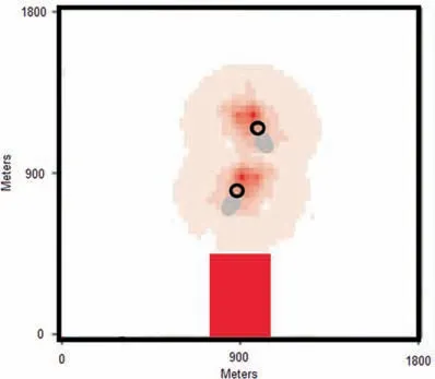
Fig. 11 Scenario 5: Initial conditions for wild-fire in second scenario.

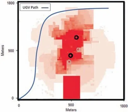
Fig. 12 Scenario 5: UGV path calculated using UAV/UGV method with the of wild-fire estimation at t=400 time steps.

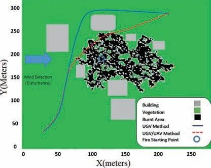
Fig. 14 Scenario 6: UGV path calculated using UAV/UGV method with the of wild-fire estimation at t=120 time steps.

5. Conclusions

In Eq.(39),Υx∈[0，1 ]is a random variable that pushes the fire in positive values in x direction through the urban environment.Since modeling the buildings in fire propagation is out of scope of this paper,we have considered the urban environment as lack of vegetation in the model. The Fig. 14 represents the details of this scenario. The UAV parameters are the same as the previous scenarios.

As it can be seen from Fig. 14, the UGV path obtained without collaboration (UGV method) represents a safer path obtained at sacrifice of time and distance reach to the goal position. This happens because of lack of update of information that leads to more conservative path. The UGV path obtained via collaboration (UAV/UGV method) is more optimal as well as safe,since it uses updated information obtained from UAV.

This paper, focuses on the implementation of a space-time Kalman filter for computationally efficient, real-time wildfire monitoring and estimation. The novelty of this work lies in the development and implementation of an estimation framework incorporating a theoretical fire growth model based on coupled partial differential equations into a space-time Kalman filter, for state estimation in the presence of noisy measurement information. To this effect, Proper Orthogonal Decomposition methods are incorporated for use with the spatio-temporal filter for achieving reduced dimensionality in computations for real-time deployability. The proposed space-time Kalman filter is then used to obtain the paths of UAV or UGV using the proposed PDE based method. The proposed method has the ability to accept and assimilate partial information gathered from UAV in making future predictions. The significance of this approach is demonstrated using simulation studies carried out where it is shown that the proposed method can reduce the risks to UGVs due to fire in a significant manner.

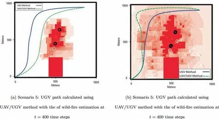
Fig. 13 Results for simulation of Scenario 5: Complex environment.

Declaration of Competing Interest

The authors declare that they have no known competing financial interests or personal relationships that could have appeared to influence the work reported in this paper.

Appendix A. Proof of Theorem 1

The optimal path is computed on a regular (x，y ) grid where elevation is added to the z component. As required from acceptable numerical solutions, the error needs to be quantified and proven to be the negligible. The Poisson problem can be derived from Eq. (34) to reduce the effect of the quantified error by considering constant permeability (e.g., κ=1)on domain Υ and is considered in Eq.(A1).

The error is evaluated, without losing the problem’s generality, by solving the equation in a two dimensional domain.

Eq. (A1) is transformed by using Green’s Relation for the Laplacian and an arbitrary test function B can be written in Eq. (A2).34No pressure gradient is assumed in y direction.

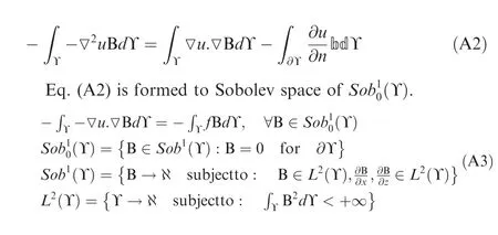
This problem formulation is transferred into a reference domain as u(x，z )→^u(ζ，η ) where (ζ，η ) represents a point in the reference domain ^Υ. Gradient of the flow in the reference domain can be calculated as Eq. (A4).

where:

The variables are transformed to the reference domain using a Jacobian transformation matrix. We define matrix G in Eq. (A6).

By using matrix G, Eq. (A3) is combined with (A6) and rewritten as:

The variable I is defined as Eq. (A8).

Eq. (A9) represents the mapping function used for transforming the data to the reference domain.

In Eq. (A9), g ∈C1(Υ ) is the geographical profile and is assumed to be continuous. The following equation is a result of implementing the mapping function on Eq. (A7).

The integral function of Eq.(A7)are emphasized due to the contribution of the topographical function g. By considering g=0 as a flat surface, Eq. (A10) can be written as Eq. (A11).

Eq. (A12) defines the error in the numerical solution.

Eq. (A12) can be written as Eq. (A13).

As it can be seen in Eq. (A13), the following result can be found:

This equation shows the result of the algorithm and provides the sufficient proof to the theorem. In this case, the method gives us zero error as g ≅0 and g′≅0.From this theorem, it is clear that the result of implementing a non-smooth topographical map (g′≫1) causes Δ ＞1, which is undesirable.50