An analysis and enhanced proposal of atmospheric boundary layer wind modelling techniques for automation of air traffic management

Jesu´s GONZALO, Diego DOMI´NGUEZ, Deibi LO´ PEZ,Adria´n GARCI´A-GUTIE´ RREZ

Aerospace Technology Research Group, Universidad de Leo´n, Campus de Vegazana s/n, Leo´n 24071, Spain

KEYWORDS Air traffic automation;Atmospheric Boundary Layer (ABL);Aviation weather;Data assimilation;Wind forecasting

Abstract The air traffic management automation imposes stringent requirements on the weather models,in such a way that they should be able to provide reliable short-time forecasts in digital formats in almost real time.The atmospheric boundary layer is one of the regions where aircraft operation and coordination are critical and therefore atmospheric model performance is also vital.This paper presents conventional and innovative techniques to improve the accuracy in the forecasting of winds in the lower atmospheric layer, proposing mechanisms to develop better models including deterministic and stochastic simulations.Accuracy is improved by optimizing the grid,assimilating observations in cycling simulations and managing a number of ensemble members. An operationdriven post-processing stage helps to incorporate detailed terrain definitions and real-time observations without re-running the model.The improvements are checked against mesoscale weather simulations at different scales and a dedicated flight campaign.The results show good performance of the model without sensitively increasing the required throughput.

1. Introduction

Growing air traffic,and subsequent air space congestion problems, have prompted a research effort to increase the level of automation of Air Traffic Management (ATM). Several approaches have been proposed with the aim to improve the efficiency of the ATM,maximize its capacity,minimize delays and environmental impact, and improve system reliability.1,2All these systems, regardless of their nature, require to estimate and predict real-time network conditions and generate consistent, anticipatory route guidance.3When ATM is referred to,this goal cannot be properly achieved without an appropriate knowledge of the atmospheric and weather conditions,in particular the wind fields.

Weather consistently generates around a third of all ATM delay in the European network,with weather-related problems increasing in recent years.4Furthermore,wind conditions have the potential to notably penalize fuel consumption (e.g. head winds that increase flight duration or storms that require route modifications). However, the impact of weather conditions on flight operations will fully arise once the currently emerging commercial UAS (Unmanned Aerial Systems) activities become fully operational.5This will not only produce an important increase in highly automatized flight operations,but also make the airplanes themselves more sensitive to wind conditions.This is due to their lower size and flight speed,and also because they mostly operate in the lower part of the atmosphere(the Atmospheric Boundary Layer or ABL),where it is more difficult to produce reliable, accurate enough, forecasts.

The ABL is the region of the atmosphere that is closest to the Earth’s surface. Its depth ranges from just a few meters to several kilometers depending on the local atmospheric situation. In our opinion, the appropriate modeling of the ABL flow is a key factor to generate weather forecasts useful for the future highly automated ATM.

Two main problems arise in studying the ABL:its complex mathematical description and the difficulties in its measurement.6The ABL in stationary conditions has been generally modelled within the first 30 to 60 m above ground level by Monin-Obukhov theory and scaling laws.7However, more advanced techniques are required in the case of higher levels,complex terrain or non-stationary studies.7

Reynolds-averaged Navier-Stokes (RANS) codes are still used as a robust and reliable tool to simulate the atmospheric boundary layer in complex terrain.8RANS studies focus on the effects of structures,9the air pollution dispersion and dilution,10and wind energy.11

In the last few years, LES simulations have proliferated,including fundamental studies of the ABL over rough surfaces,12urban canopies13and their application to wind energy harvesting.14The simulations typically use pseudo/spectral and finite-difference solvers,with special focus on parallel computing.15Three lines of research can be found:1)subgrid models to study the effect of the unresolved scales of motion,162)wall models17and 3) the implementation of robust numerical schemes.18

Numerical simulations need to be complemented with field measurements and wind tunnel experiments.19The latter usually try to simulate the neutrally stratified boundary layer,modeling the turbulence scales,the mean velocities distribution and the energy spectrum.20Great efforts have been made to study the complex unsteady wind configurations,21the flow separation and reattachment,22and urban areas.23

Relative to field measurements, sounding balloons, sonic anemometers and other fast-response sensors have been traditionally used to derive ABL properties.6In recent years, the relevance of alternative remote sensing instruments has grown such as in the case of satellite scatterometers,24UAS25and platform-based light detection and ranging (LIDAR), both over land26and sea.27Micro-pulse LIDARs have been recently deployed to study the aerosol vertical structure28and shortterm ABL evolution.29

This paper firstly reviews the tools currently used to forecast weather conditions (with special attention paid to the ABL modelling and the wind fields) and how the available meteorological information is disseminated to support ongoing flight operations. Once the necessity of new approaches for aviation weather data is presented, we propose the implementation of different improvements that entail not only with numerical prediction, but postprocessing and dissemination.The suitability of the suggested methodology and software tools is then tested by performing a dedicate flight campaign,whose results are briefly presented.

2.Generation and dissemination of aviation weather information

The International Civil Aviation Organization(ICAO)and the World Meteorological Organization (WMO) have established international standards to ensure high-quality meteorological reports.30Those reports mainly rely on the results from state of the art Numerical Weather Models complemented with insitu measurements.

2.1. Weather forecast models

Modern weather forecasting relies mostly on numerical models that simulate the evolution of the atmosphere, based on fluid dynamics and thermodynamics equations.31When specifically referring to the ABL,and because of the complexity of the processes taking place there,it is very difficult to formulate a numerical model capable of reproducing all of them accurately.

Apart from the influence of the synoptic tendencies, the ABL is influenced by a significantly large number of smallscale features that are very difficult to capture in a numerical model where space and time resolution are limited. This becomes especially true when an operational model is pursued and tradeoff resolution quality is required for shorter processing time.31Modeling the eddy transport and vertical fluxes that occurs in the ABL requires a very fine grid,but these grids are not affordable for a mesoscale numerical model. This is why special techniques have been developed in order to handle these processes in the ABL.

Specifically,ABL schemes are implemented in the numerical meteorological codes.The ABL schemes are in charge of the calculation of the flux profiles within the well-mixed boundary layer and the stable layer,and thus provide atmospheric tendencies of temperature,moisture(including clouds),and horizontal momentum in the entire atmospheric column.The schemes are one-dimensional,and they assume that there is a clear scale separation between sub-grid eddies and resolved eddies.This difference is more difficult to see when grid sizes are below a few hundred meters, where boundary layer eddies may start to be resolved. In these situations, the one-dimensional scheme should be replaced by a fully three-dimensional local sub-grid turbulence scheme such as the TKE diffusion scheme.32Such kind of meshes can also be resolved making use of Large Eddy Models that will be discussed later.

ABL models can be divided into two big groups33:

(1) First-order closure schemes. They do not require any additional prognostic equations to express the effects of turbulence on mean variables. Most popular models are MRF34, YSU35and ACM2.36

(2) One-and-a-half order closure schemes (also known as TKE closure schemes). They require one additional prognostic equation of the TKE. Some well-known models are MYJ37, QNSE38, MYNN39and BouLac.40

2.2. Meteorological services for air traffic management

Meteorological services for civil air traffic are regulated by ICAO Annex 3 - Meteorological Service for International Air Navigation. Each member state of the organization is responsible for establishing the meteorological services meeting the operational needs described in the aforementioned Annex 3.41These products can be grouped in three categories42:

(1) Observations. METARs (METeorological Aerodrome Reports) are a report of current weather conditions at an airport.

(2) Forecasts. They can be divided into two categories,those provided for a single aerodrome site and those provided for an area, region or route.

(A) Aerodrome Forecasts: TAFs are forecasts issued for a given aerodrome at a specified time, which contains a concise statement of the expected meteorological conditions. Landing Forecasts or Trends are a forecast appended to the METAR including some details about the expected changes in one or more of the elements.

(B) Area and Route Forecasts: Forecasts of the meteorological conditions which are expected over an area or route are generally referred to as AIRMETS or GAMETS. They are usually provided for a specific Flight Information Region(FIR).

(3) Warnings. They provide information about specific meteorological phenomena that imply risks for aviation.They are the SIGMETs (short period warnings of hazardous weather expected to affect aircraft in flight within a specific area or FIR),Aerodrome Warnings(meteorological conditions which could adversely affect aircraft on the ground and aerodrome facilities and services)and Wind Shear Warnings(information of the observed or expected occurrence of wind shear).

However, these meteorological services provide a limited amount of information and are not enough for all the modern requirements of new Air Traffic Management (ATM) concepts. Efforts in Asia, Europe and North America to streamline ATM to permit greater capacity and efficiency demand improved meteorological services.43

To address modern requirements for ATM-specific weather services, the World Meteorological Organization (WMO)Commission on Aeronautical Meteorology(CAeM)is defining the gaps between information provided by legacy products and information required by current and emerging needs to develop a prototype for improved meteorological services.

It is clear that a demand exists for new products that better serve the needs of the global aviation community for accurate and timely weather information, including wind field.

3. Discussion on some improvements for generation of aviation weather data

The need for higher resolution forecasts has historically driven numerous methodologies to generate more detailed outputs.44Different possibilities, that were applied to the model developed by the researchers, are now discussed and organized in three groups: those to be applied to the NWM itself, to the output postprocessing and some other off-line improvements.

3.1. Improvements on numerical models for wind forecasting

3.1.1. Grid selection

Grid resolution needed to accurately reproduce flow state properties is strongly related with the rate of change of such properties. When the value of a certain parameter quickly decreases or grows, a finer mesh is needed in order to have a sufficient number of points to sample such changes. This happens in the ABL,where flow variables notably change within a relatively very short distance.

Many regional model simulations make use of a vertical grid system of 28 levels with the model top located at 50 hPa.33When applying this vertical resolution,there are nine layers below 2000 m. The lowest level above the ground is 0.990 (pressure level) and the first mass point is located at approximately 40 m.

Increasing the total number of vertical levels allows researchers to improve the resolution at the bottom of the boundary layer. By defining 37 vertical levels, the first mass point is located at about 10 meters and there are 17 layers below 2000 m.

3.1.2. Implementation of LES techniques

Another way to improve the accuracy of the forecast is increasing the horizontal resolution of the grid that is being used for the calculations.The resolution commonly used by the numerical weather prediction models usually ranges from 200 km or above in the global or synoptic models and between 2 and 200 km for the mesoscale models. When moving to grid resolutions notably lower than 2 km, a new technique for turbulence modeling should be applied. It is known as Large-Eddy Simulation(LES)model.This model explicitly resolves the largest scales of the turbulence,something only feasible when the resolution of the grid is sufficiently large. The implementation of the LES model is very demanding in terms of computational power and it is still far from operational applications.

LES is capable of achieving a better performance,for example when investigating45:

(1) The dynamics of convection in the ABL and convective clouds and rainfall.

(2) The impact of urban areas on the microclimate.

(3) The influence of abrupt changes in the local landscape and land cover on atmospheric flows and landatmosphere exchanges.

It is obvious that, by increasing the horizontal resolution,the number of terrain features that are modeled by the software increases.This approach has a higher computational cost as a consequence of two issues: on the one hand, the higher number of grid elements that are required and, on the other hand, the higher complexity of the equations to be solved for the LES model. These costs are clear and obvious; however,there are also some hidden costs that should be faced in order to achieve better accuracy:new high-resolution data should be provided for vegetation/soil/land use, soil moisture or topographic shading. This is especially important for complex terrains where the characteristics and properties of the terrain change notably in short distances.

3.1.3. Local data assimilation

Assimilation of observations is a widely used technique in order to improve forecast accuracy. Observations of the current, or past, state of the atmosphere are combined with the results from the model to produce a new forecast,which is considered as ’the best’ estimate of the atmosphere conditions at the analysis time. The increasing availability of observations,in terms of coverage and refresh time,has notably contributed to improving the forecast accuracy during the last decade.

The same principle can be applied to the atmospheric boundary layer. Such measurements can be obtained using towers, tethered balloons, and manned or unmanned airborne systems. Since aircraft travel over large distances in comparatively short time,airborne systems are able to take a‘snapshot’of the atmospheric flow.Length scales between convection and small scale turbulence are covered. For that reason, airborne measurements are a good supplement to ground-based measurements and remote sensing.46Different systems have been developed for that, such as the manned research aircraft CASA-212-200(INTA),the helicopter-borne turbulence probe Helipod47and the Unmanned Aerial Vehicle (UAV) named Meteorological Mini Aerial Vehicle (MMAV).46

3.1.3.1. Discrete or continuous data.

The measurements collected by these methods can then be used to improve the forecasting process. They are assimilated into the numerical model by means of different techniques:empirical methods (nudging), statistical methods (variational data assimilation) and advanced methods (Kalman filter)

Newtonian relaxation, also known as Four-Dimensional Data Assimilation(FDDA) or just Nudging,does not employ statistical methods in order to define the most probable state,but forces the model to modify initial state values in order to bring them nearer to the obtained observations.

Variational (Var) data assimilation combines observations and forecasts through the iterative minimization of a prescribed cost (or penalty) function. Typically, the cost function is defined as the sum of the squared deviations of the analysis values from the observations weighted by the accuracy of the observations, plus the sum of the squared deviations of the forecast fields and the analyzed fields weighted by the accuracy of the forecast. Differences between the analysis and observations/first guess are penalized(damped)according to their perceived error. This ensures that the analysis does not move too far from observations and forecasts that are known to be reliable. It can be applied in two different ways:

(1) 3D-VAR. It combines all the available information about the atmospheric conditions in a certain period of time(T-1 to T+1 in Fig.148,where T is the analysis time) and they are treated as if they were at T+0 which is close to their average time.

(2) 4D-VAR. The variational analysis compares observations with background model fields at the correct time and combines observations at different time during the 4D-VAR window in a way that reduces analysis error.

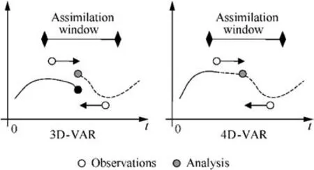
Fig. 1 Differences between 3DVAR and 4DVAR (Adapted from Barker et al.48.

Kalman filtering has been the last tool incorporated into meteorological forecasting, becoming a relevant one for mesoscale model initialization by means of data assimilation.Kalman filter performs an analysis at each timestep of the(discrete)model,using only the observations available during that timestep.Fig.248shows the differences between Kalman Filter and 4D-Var method. Two main Kalman filter methods have been developed: the Ensemble Kalman Filter, that generates the most probable atmospheric state according to the uncertainties associated with available measurements as well as those associated with the atmospheric state,and the Ensemble Transform Kalman Filter, similar to the previous one but, in this case,covariance matrix that determines the level of uncertainty in the system is also propagated at each iteration.

3.1.3.2. Usage of historical data.

The execution of variational analysis requires a certain number of historical forecasts to compute what is known as the background error of the model. Background error covariance statistics are used in the variational analysis cost-function to weight errors in features of the background field.The assimilation system will filter those background structures that have high error relative to more accurately known background features and observations.49

One common method for the estimation of climatological background error covariances is the NMC-method. In this process, background errors are assumed to be well approximated by averaged forecast difference statistics (e.g. monthlong series of 24-12 h forecasts valid at the same time).

3.1.4. Simulation cycling

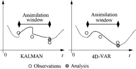
Fig. 2 Differences between Kalman filter and 4DVAR.(Adapted from Barker et al.48.

When dealing with short propagation intervals from real time(also called nowcasting or short term forecasts), the model should be initiated at a former time to allow for system stabilization and to be able to assimilate known measurements.Thus,the simulation is composed of two stages:the first driven by assimilated data and a second of free running propagation.Once the simulation is completed, the results are ready for usage along the forecast interval; however, as time passes,new observations may be available.

Adapting the forecasts to the new measurements could lead to solutions not compatible with the physical weather models.Depending on the nature of the observations and the particular applications of the final products, this option could be of interest.

A more elaborated technique implies re-running the model every time new observations are available. Obviously, the excessive frequency may lead to invaluable redundant forecasts with high computational effort.Moreover,the second and following runs may take initial conditions from their own generated products instead of coming back again to global model data (that would otherwise be likely to remain unchanged).This mechanism is called simulation cycling.

In recent years, nudging assimilation has shown good performance for short term forecasts. Discrete variational assimilation is slightly costlier, but more versatile as observations are interpolated to forecast time. However, the stability of the simulation may suffer,especially during the first simulated intervals. Finally, continuous variational assimilation is computationally intensive.

The implementation proposed in this article is based on nudging assimilation and simulation cycling as can be seen in Fig. 3. In this way, the atmospheric model is developed in three different stages:

(1) Preparation of initial and boundary conditions from global models, generating a baseline sequence for the whole interval of interest

(2) A first simulation assimilating all measures up to the model’s initiation and generating the atmospheric status at the initial time

(3) Simulations started at baseline times, using the baseline forecasts as the initial condition, assimilating the observations available at those times

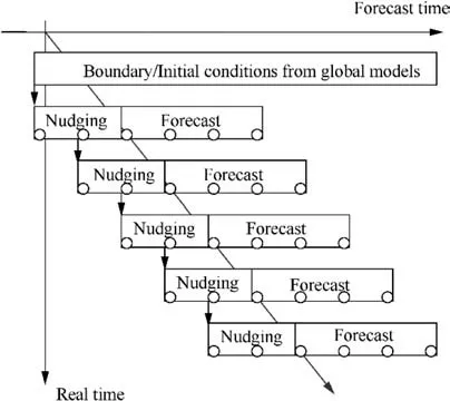
Fig. 3 Simulation cycling scheme.

The nudging parameters allow the tuning of observation propagation in space and time.With respect to the space propagation, horizontal influence may depend on the homogeneity of the terrain(relief and radiometry).Vertical coupling follows similarity theories in atmospheric boundary layers. Recent papers50provide some rules to tune time persistence parameters in combination with other model configurations.

3.1.5. Ensemble forecasts

Once a propagation model has been setup, an obvious technique to extract more information from it consists of running it multiple times with slightly different configuration parameters or initial/boundary conditions.This is known as ensemble forecasting. If multiple simulations produce very similar results, forecast confidence levels may be considered higher.Of course, the nature of the perturbations introduced in each of the ensemble members is crucial to make this consideration true.

When configuration parameters are changed, all the elements discussed above are valid. However, the simulation cycling provides a natural mechanism of ensemble generation as, in every cycle, new observations are assimilated during the nudging stage and hence the model forecasting interval starts with different conditions from previous runs.In the current concept, boundary conditions are kept constant during longer time but they could also be included in the cycling.

As the campaign progresses,new members are added to the ensembles up to a maximum given by the number of outputs in the forecasting stage(Fig. 4)and decrease with forecast times.Should a more homogeneous ensemble forecast be required,forecast stages of each cycle can be extended to the campaign end time, producing ensembles with a stable number of members (Fig. 5).

The members of the ensemble do not need to have the same weight in a hypothetical summary forecast.It seems reasonable to have greater confidence in recent simulations, including recent observations,than in old runs.Thus,a weighted average forecast could be a good representation of the atmospheric status at a certain point in time.

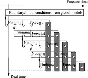
Fig.4 Heterogeneous ensemble forecast made of multi-temporal simulations.

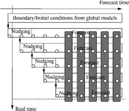
Fig.5 Homogeneous ensemble forecast made of multi-temporal simulations.

The weight distribution could also be changed for successive forecast times.For example,when interested in immediate atmosphere variables, the last run can provide better captures of fresh observations, but for further forecasts, weighting can be more homogeneous so that very recent variations could be temporal or local and not so relevant in the future. For the sake of clarity, this scheme of weighting is shown in Fig. 6 for an ensemble generated in successive hourly simulations run from 9:00 h to 14:00 h, and composed final forecast products from 14:00 h to 22:00 h. For short term forecasts, recent simulations are more relevant, whereas for mid-term products the weights are more uniform.

3.2. Forecast data post-processing

Some improvements are also proposed,which does not involve the NWM itself, as they deal with the outputs of the model.Numerous methodologies for statistical downscaling based on different, and usually complex, principles have been proposed: analogues,51interpolation52or machine learning models.44We propose an interpolation technique specifically developed to maximize data accuracy within the ABL.

After the successful execution of mesoscale weather models,three problems arise for interpolation during post-processing:

(1) How to vertically interpolate wind values among grid points, especially in the ground contact cells

(2) How to adapt the grid-based data to a more detailed terrain model, typically available at local domains

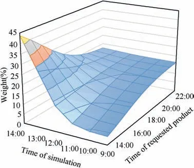
Fig. 6 Proposed relative weighting of forecast members among recent and past simulation for various future forecast time.

(3) How to horizontally interpolate from grid points to generic points using that detailed model

The decoupling of horizontal and vertical interpolations responds to the existence of a privileged direction following the gravity force. The boundary layer approximations and the adaptation of real terrain height affect only this direction.The right order in which vertical and horizontal interpolations are performed is not a priori obvious, and requires some discussion.

3.2.1. Vertical wind interpolation at surface layer

The similarity theory provides an acceptable way to interpolate wind speed values in the surface layer in the form:

where Uwis the wind speed modulus,u*the friction velocity,h the geometric height above ground, k the Von Karman constant (usually taken between 0.35 and 0.4, regardless of wind flow or surface), z0the roughness length and ψ the stability correction term that can be derived from Ref.53as a function of the height relative to the Obukhov length (L).d0is the displacement height, very useful to cope with the existence of ground structures that elevates the zero-wind level above the zero-height reference. It may be used to adapt the weather model terrain data (mesoscale grid) to a more detailed digital elevation model

For the bottom first cells, exceptional operations may be required. The model results provide data at height-center of the cells.That means that the first data is several meters above ground.Regardless of other data provided by the model,a neutral surface layer can be considered to reasonably interpolate data within the first cell.In the case of wind speed,two extra considerations apply when considering Eq.(1),that includes three unknowns(z0and d0dependent on ground and streamline history and u*dependent only on air flow)and hence several matching points are needed(Fig.7).Zero wind is achieved at a height of z0+d0,being the usual roughness length quite small(much less than 1 m in airport-like flat areas).

Moreover, change in wind direction between the two first cells is normally small, so that the profiling can be performed with the modulus of the wind estimates given by the mesoscale model. The wind direction can be interpolated to ensure continuity of the wind profile with altitude.

3.2.2. Adaptation to detailed terrain models

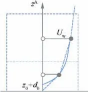
Fig. 7 Scheme of log wind profile in bottom boundary cells.

Regarding the second point, topographical features captured by mesoscale models are much rougher than the usual terrain maps available for local domains(Fig.8).This introduces sensitive errors if the point of interest is given by its height above the real terrain and injected in the mesoscale grid. Sometimes this can provide unrealistic results as they correspond to points situated under the ground surface;in other cases,large inaccuracy may exist because wind velocity changes quicker with height in the surface layer region.

The first method to adapt the vertical profile to the real terrain altitude is to solve the wind logarithmic vertical function by forcing the new altitude into d0and then using two known wind values (U1and U2at h1and h2respectively):

Fig.9 represents a reference line for the wind speed in a real(and characteristic)case where first cell is located at 10 m over the terrain and second one around 35 m.If a more detailed terrain definition confirms that ground level is+2 m from that reference, a new curve is provided. The problem arises when the mismatch between mesoscale ground reference and the new relief is close to (or larger than) the first cell position.Fig. 9 also plots the error between wind reference and the adapted curve. Maximum values of 5% are possible only if the terrain difference is lower than 80% of the first cell center height (+8 m in this case).

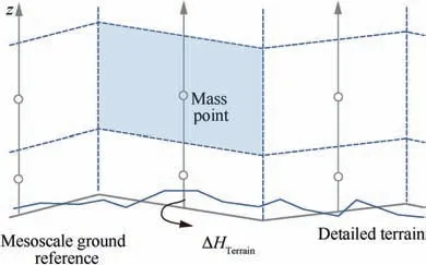
Fig. 8 Scheme of detailed terrain model on top of grid.

When the new reference is high enough to make the first cell point unusable,the next two points may be used.In that case,the errors with respect to the initial reference may turn out to be unacceptable. Better results are achieved if a roughness length is assumed and a single matching point used. The estimated z0can be calculated from the reference mesoscale curve,Eq.(2),as the land use and streamline paths are kept.Updated curves are shown in Fig.9(b),where error is calculated for the first curve that uses a single matching point. Relative error reaches 10% close to the detailed terrain height but decreases very rapidly with altitude.

Another completely different way of adapting the existing meteorological mesoscale data to detailed terrains is moving the whole curves in the vertical axis. In order to minimize the errors in the interpolation mechanisms, but without running a new simulation with a more detailed terrain model,the terrain-following hydrostatic pressure level η can be used for the vertical coordinate.54

where Phdenotes hydrostatic pressure and TOA stands for the top of the atmosphere.Thus,for a vertical grid line such as the one shown in Fig. 10, the vertical position of the cells is given by their η level. If a mismatch exists between mesoscale and local terrain models, vertical values of atmospheric variables may require some kind of correction to meet basic physics laws such as hydrostatic forces or mass conservation, as proposed in the following paragraphs. Given a result of the mesoscale model,pressure,temperature,wind speed and turbulent kinetic energy are estimated as a function of η all along the grid points of the domain. The inverse is always possible and η can be derived when a pressure or geopotential height is given, as these functions are monotonous. Let us add an asterisk to the variable names corrected for fluctuations in terrain altitude with respect to the mesoscale reference (ΔHTerrainin Fig. 8).

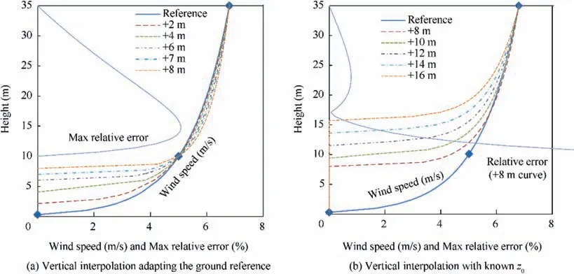
Fig. 9 Logarithmic interpolation at lower cells using two matching points and refined ground references above the original one and using one matching point and an estimated roughness length.

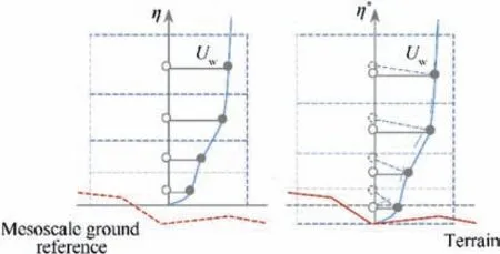
Fig. 10 Scheme of wind profile matching to terrain model.

As explained before, the wind profile within the surface layer is dependent on the wind values given by the model in the bottom first cells. Furthermore, wind speed gradient is large in this region,and therefore,sensitive errors may appear if the terrain reference is changed carelessly.

The original cells are defined by the terrain-following η levels.Considering low slopes with land homogeneous properties,the boundary/surface layer could be fully developed along the upstream air flow, and thus it can be considered that the vertical wind profile, upwards from ground, is almost unchanged(Fig.10).This means that it is reasonable to adapt the original wind profile to the new terrain reference by using the η*parameter in a similar fashion to the temperature correction.

One could think of this as violating basic mass conservation laws. A more detailed correction can include a wind modulus increment/decrement that compensates the slight change in cell height due to the use of η*levels instead of η levels.In practice,a bottom cell of 20 m height,when a positive terrain mismatch(ΔHTerrain)of 100 m is present and the atmosphere top height is 20 km, shows a change of only 0.5%, that would be the error induced to the uncorrected wind speed, being well within the wind speed error of mesoscale outputs.

Thus,a good estimate for the pressure is the same given by the model, extending the data along possible terrain depressions using the hydrostatic law (in other words, allowing η to take values lightly larger than 1). It can be written as

On ground, the pressure expression would be:

where Ra=287J/kg·K is the ideal air constant and air conditions at η=1 are the surface values on the mesoscale terrain.Following this approach,a corrected η*level can be defined as

Now, new temperature and wind profiles can be obtained by re-scaling the original model using the corrected input variable to consider the new terrain altitude.This modifies the temperature field maintaining the ground temperature given by the mesoscale analysis.

Now, new temperature and wind profiles can be obtained by re-scaling the original model using the corrected input variable to consider the new terrain altitude.This modifies the temperature field maintaining the ground temperature given by the mesoscale analysis.

3.2.3. Horizontal interpolation

Conventional consideration in horizontal interpolation processes is the mathematical interpolation method to get the value of a 2D function given three or more known values at known points. Some of the available interpolation methods include four-point bilinear,sixteen-point overlapping parabolic,simple or weighted four-point average, simple or weighted sixteenpoint average,nearest neighbor,breadth-first search(or nearest valid neighbor)and model grid-cell average(used when data resolution is higher than grid domain resolution).

When considering the use of a terrain model that is more detailed(and mismatching)than the mesoscale grid,other side effects are related to the order in which vertical and horizontal interpolations occur. Horizontal grid spacing is normally constant,so the access to the proper cell(and neighbor identification) is trivial. However, vertical levels are not iso-spaced,which implies that:

(A)Horizontal/vertical:horizontal interpolation provides a new profile that can be easily used for vertical interpolation and terrain matching. This obvious procedure presents the problem that,for a single request,the horizontal interpolation of all the height levels(of the four grid neighbors)is necessary previous to the vertical interpolation. This is because there is no a-priori information about the vertical level required, and a further iteration on the interpolated data is necessary. In other words, η*is unknown in the target point and does not necessarily need to be equal than the ones in the corners. All this decreases the agility of the algorithm.

(B) Vertical/horizontal: vertical interpolation can be first executed on the four nearest neighbor grid points, with each one adapted to the real terrain height. Then, the horizontal averaging can be performed. This mechanism is lighter than the previous one. However, as the terrain height of the point of interest is not used,it could provide bad results in unfavorable cases such as the surface layer shown in Fig. 11, where inner terrain is higher than the one at grid points.

In principle, the horizontal/vertical scheme is preferred. If data access speed is a driver, a trade-off solution could be to use a vertical/horizontal scheme but considering that, for the four corners, ΔHTerrainis one of the requested points. This ensures there is no underground outputs and the surface layer consistently matches the terrain height (Fig. 12).

3.3. Other offline improvements

Finally,another method known as real time re-analysis is proposed to improve the accuracy of the wind forecast products with no need of additional executions of the model. Weather model cycling is able to ingest current observations in the model,as pointed in Section 3.1.4.Unfortunately,the process requires to run again a full simulation and makes it impractical.Alternatively,there are ways to embed fresh observations directly into the final products, assuming they are close to predicted values and thus they can be considered as small perturbations in the variable fields.A clear example is the case in which an airplane is flying following a programed path within the estimated wind field. As part of the flight instruments, airspeed and ground speed are always measured and monitored.It could be interesting to use the real-time in-situ measurement to improve,at least locally and momentarily, the wind field estimate. The same is applicable to other atmospheric variables.

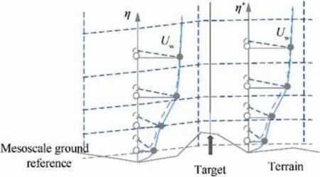
Fig. 11 Scheme of vertical/horizontal interpolation with problems to adapt detailed terrain model to existing grid profiles.

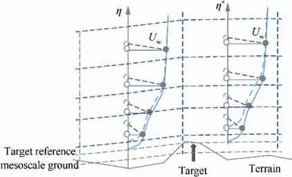
Fig. 12 Scheme of vertical/horizontal interpolation with height corrections at grid points taken from target point.

Nudging is a common practice in quick observation assimilations. Good results have been obtained from comparative re-aliases exercises. Trying to keep the physical meaning of the perturbations, temperature nudging can be performed in a conventional way(Fig.13)that resembles a local atmosphere heating due to whatever reason. Delta pressures, however, are more delicate as pressure gradients have a relevant impact on wind fields. Considering that this is a post-processing correction,it seems reasonable to embed pressure as an extra hydrostatic delta pressure affecting the whole vertical profile.

If this approach is too aggressive (even ground pressure is affected), a relaxation factor can be included to moderate the effect. For local effects, pressure nudging should be executed in a way that does not permit larger pressures at higher regions within the same vertical profile (Fig. 14).

Wind velocity is responsible for advection of fluid properties.This transport mechanism is more efficient than diffusion,and hence it is quicker.This allows the development of a more complex set of procedures for real-time nudging of fluid internal properties in which the local velocity is considered to guess the impact of a given observation, both in space and time.Apart from the nudging scale that normally depends on the 4D distance to the observation point/time, this distance can be measured along the trace of the particles.

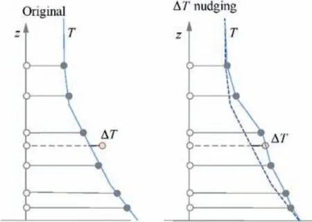
Fig. 13 Scheme of post-processing temperature nudging.

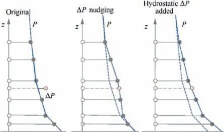
Fig. 14 Scheme of post-processing pressure nudging.

In order to seamlessly integrate the velocity measurements,it would be interesting to fulfill the mass conservation constraint. This is difficult as soon as observed velocities differ from the ones expected by the model. A nudging function is proposed to add changes in wind velocity Δ=(Δuw，Δvw)in the North direction:

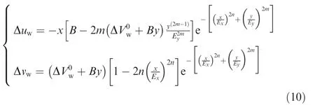
The above process allows for the inclusion of a single recent observation in a final product. When several of these observations are available,weighting factors can be used to avoid over constraining of the assimilation problem.

4. Operational validation

4.1. Architecture and model implementation

A dedicated testbench named Atmospheric Model has been built to validate the performance of the proposed forecasting methodology and to serve as a precursor of the final system.The testbench includes (Fig. 15):

(1) The ensemble-enabled Numerical Weather Model based on the open-source widely validated WRF code

(2) A scheduler module

(3) A database with the available observations

(4) A database with the resulting files and comprehensive logging architecture for all the processes

(5) An Application Programming Interface(API)with a set of functions implementing data access algorithms with the improvements presented in this paper related to terrain matching and data interpolation.

(6) A simple viewer software to visualize the forecasts and to allow tabulated outputs (wind profiles, horizontal cuts, streamlines, iso-level lines, etc.)

Data produced and updated regularly are timely served to operators through a client-server architecture using CORBA middleware.A publishing/subscribing procedure is used to distribute the products among the active users. In order to save communication bandwidth, the transactions are designed to mount meteorological hyper-cubes at client side in a progressive way. A dedicated Application Programming Interface(API)has been produced to access the data in a quick and efficient manner from most of common computer languages.

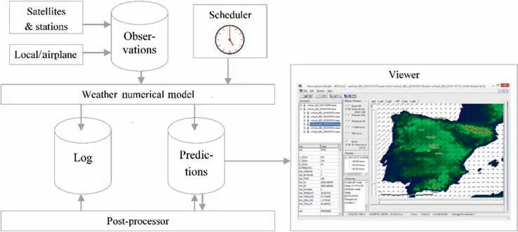
Fig. 15 Model architecture.

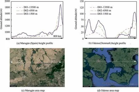
Fig.16 Ground altitude profiles as seen by mesoscale NWM for each domain:D01(cell size 13.5 km),D02(cell size 4.5 km),D03(cell size 1.5 km).

4.2. Results

In order to check the accuracy of the proposed methodology implemented in our Atmospheric Model,tests have been developed on two sites of very different orographic characteristics:Odense airfield,in the Danish Fionia island and Maruga´n airfield in a mountainous region close to Madrid, Spain. WRF model is run with three nested domains (European level at 13500 m resolution [D01], regional level at 4500 m [D02] and local level at 1500 m [D03]). Each domain sees the terrain at different definition levels (Fig. 16) which obviously results in differences for the vertical profiles of each variable at a given location (the airfields located at Maruga´n in Figs. 16(a)-(c)and Odense in Fig.16(b,d)).Six ensemble models are launched every hour (Fig. 17).

Regarding wind intensity,a relevant variable for ATM,differences in grids sizes tend to produce misalignment in wind profiles. In some occasions, coarse resolution models tend to clearly underestimate wind strengths whereas in others the overestimation is almost negligible. The impact is quite well correlated to the type of terrain and the variability of the ground slope pattern.For example,in low altitude Odense site the boundary layer profiles are quite independent from the grid size selected, whereas in the mountains of Maruga´n this parameter is a result driver.

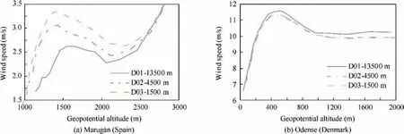
Fig. 17 Wind profiles forecasted by mesoscale NWM at each domain for ABL (2 km height).

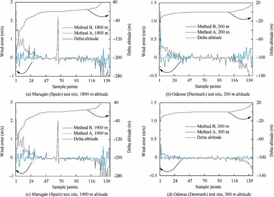
Fig. 18 Comparison between ground altitude correction methods A and B at 144 test locations around test sites.

With this data, an inter-model comparison is developed to check the effect of the different resolutions in the definition of the atmospheric variables in the ABL. In this test, the coarse regional model is adapted to a finer ground resolution. To do that, the terrain values of the detailed domain are used.

As defined in Section 3.2, two interpolation methods are proposed to downscale mesoscale forecasts to a better detailed terrain. They will be named as:

(A) Method A:logarithmic curve in first cells,linear interpolation for the rest

(B) Method B: re-scaled profile curves in vertical axis

At a total number of 144 test locations falling within the surroundings of each airfield, interpolation methods A and B will be used to compare the downscaled meteorological products from coarse regional domain with those originally obtained using the finest domain. Results are depicted in Fig. 18. For the sake of clarity, the samples have been sorted with respect to the difference between mesoscale terrain model and detailed height (ΔHTerrain).

Apart from the obvious dependence of the wind speed error with the correction height, the performance of method A versus method B is clearly showed. The main difference is that,close to the surface, the presence of small hills, which are not captured by the coarse grid, produces a correction towards higher winds in method A and towards lower winds in method B. According to experience and confirmed by the full-physic fluid models used in the NWM, the first option is more accurate.

In order to provide a better view of this effect, the vertical wind profile is plotted at two locations close to each airfield using the intermediate and the fine domain. Then, the profile of the single cell in the coarser domain can be compared to the corresponding nine cells in the second domain (see Fig. 19). In the Odense plot, where ΔHTerrainis about 20 m, it is well recognized that,from the reference model,a better estimation of wind speed for a detailed terrain is obtained by moving up following the existing wind profile curve (interpolation method B) than by inventing a new re-scaled curve above the original. The Maruga´n sites present much more dispersion due to the large difference in ground altitude among the nine points, and hence the above conclusion, although also true,is not obvious.

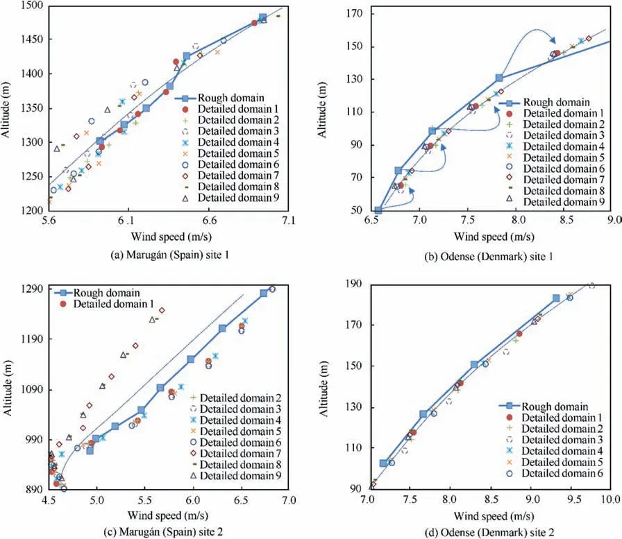
Fig. 19 Wind vertical profiles forecasted by the intermediate domain and the detailed one in two locations close to experimental sites.

Finally, last analyses focus on the results that can be achieved by our Atmospheric Model thanks to the implementation of an NWM where the different capabilities described in Section 3.1 have been used. Aiming to have near real-time wind forecasts and then provide valuable operational data for ATM automation, new forecasts are made available every hour for the next 4 hours.

The value for ATM automation of having such a high temporal resolution is shown in Fig. 20. The hourly evolution of the ABL is depicted and it is possible to identify how the wind profile changes. In this case, the boundary layer is evolving towards a narrower thickness and hence accelerating the winds close to the surface.

As to the probabilistic capability of the Atmospheric Model, Fig. 21 represents the wind speed profile in the ABL for six different versions of the same simulation, composing one single ensemble once averaged. Different physics were applied to each member, modifying the radiation model, ABL model, microphysics and cumulus parameterization. Dispersion among the models is more conspicuous in the entrainment layer, where free atmosphere fuses with terrain boundary layer (around 1000 m above ground in this example).

Finally, an additional and more detailed test is presented,simulating near real-time data assimilation. This is done using wind measurements derived from flight data collected during a test flight (Fig. 22) carried out by BRTE UAV within a flight dynamics test campaign. Site and dates are undisclosed.

Due to the high frequency of the measurements, they show a notable dispersion from the average value that is not present in the numerical forecast. They are processes to obtain timeaveraged values that could be used for the test.Wind measurements are firstly compared to the forecasts given by the model executed two hours earlier, showing a reasonable agreement(Fig. 23).Also, the execution of the model was repeated again using data assimilation from an in-situ anemometer in order to diminish the difference between the forecast and the airborne measurements, as well as to check the validity of data assimilation in the ABL. The result is also shown in Fig. 23. After data assimilation, wind velocities forecasted by the model are smaller and closer to observations (from green to blue lines).Additionally, the ensemble forecast characteristic was activated for this case, providing a range of wind estimations for each position and time of the airplane. For the 5 min flight time,a relative±3%dispersion(3-sigma)was estimated when considering equi-probable forecast members.

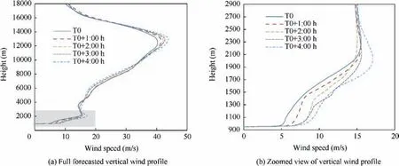
Fig. 20 Wind profile evolution along 4-hour simulation in Maruga´n for the detailed domain.

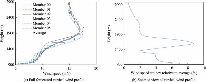
Fig. 21 Wind profile ensemble after 4-hour propagation in Maruga´n detailed domain.

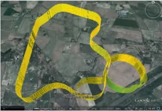
Fig. 22 Ground track and 3D view of test flight campaign (site undisclosed).

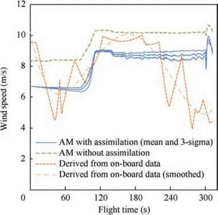
Fig. 23 Wind speed measured and estimated during test flight.

5. Conclusions

Nowadays, there is a need for modern wind models that not only focus on accuracy, but also are closer to operational needs in terms of time execution, time and spatial resolution,etc. Regarding air traffic management support, readiness of accurate 4D-digital information is of paramount importance.Moreover, given the relevance of aircraft operations, maneuvers and the required automation for UAS operations in airport areas, the performance requirements of the meteorological products in these regions are stringent. Unfortunately, the lower part of the atmosphere, the Atmospheric Boundary Layer (ABL), is the most difficult to model accurately.

(1) The first place of improvement is the selection of the grid and turbulence parameterization. The Large Eddy Simulation (LES) techniques are promising although somehow constrained from the computational point of view.On the other hand, the assimilation of observations is very useful to tune the model while it is being propagating. From simple forcing to complex Kalman filtering,this external information enables better accuracy and confidence. However, even if this approach is optimum for meteorological re-analysis (simulation of past times when observations are available), they can only serve as initial conditions when developing forecasts.To overcome this limitation, once a forecast is fully developed,the concept of simulation cycling helps to embed the atmospheric truth in the resulting products.Hot simulation runs use outputs from former simulations to deliver new products quicker. Even so, the old-fashioned data can be used within the ensemble, although with less weight in the average. A weighting function has been proposed in this work to boot recent simulations in near future forecast times.

(2) The second place of improvement has been proposed during product post-processing. Without running again the model, we propose some specific downscaling techniques based on interpolation to improve the accuracy within the atmospheric boundary layer. This vertical and horizontal interpolations should be done carefully,as they are coupled and the terrain height at the requested point does not need to be the same as the one present at grid points. The analysis showed that the proposed approach can be used successfully to match the mesoscale data to more detailed terrain definitions.

(3) Finally, real-time re-analysis is a trial to embed known variables (normally coming from local observations)into the final products without disturbing too much the essence of fluid motion laws. A way is proposed to nudge temperature and to adapt new pressure values keeping hydrostatic forces. Besides, a mechanism to include wind velocity values maintaining conservation laws is presented.

(4) These three blocks are quite independent and fully compatible when trying to improve the modelling of the ABL. While all the mentioned techniques are useful to improve the results, not all of them result equally feasible. Processing time is strongly penalized when propagating LES turbulence models and the associated highly detailed mesh. The implementation of ensemble forecasts to provide stochastic predictions can be considered a more affordable approach, as load grows lineally with the number of ensemble member. In that case it can be efficiently executed in parallel, optimizing the existing computational resources.Finally, data assimilation is a highly efficient utility to improve ABL modelling at a variety of computational costs, from virtually null if used as initial condition to quite complex variational techniques; in any case, the availability of meteorological sensors in the domain of interest can be difficult to achieve, furthermore off ground. Depending on the available resources, the techniques can be prioritized or, ideally,applied at the same time.

(5) On the other hand, the proposed post-processing techniques that define a set of interpolation rules and make it possible to match the terrain reality from rougher grids are recommended in every situation.They enhance the accuracy of the results at little cost.In particular,for the application of automation of ATM addressed in this work,a continuous and quick forecast re-analysis is proposed to embed data acquired in flight. This provides a near real-time forecast capability that offers the best performance from the available computing resources.

(6) The above concepts have been tested in several sites and atmospheric situations, providing a first-hand impression on their value. Ensemble forecasts have shown levels of divergence in the models,allowing the development of a pre-operational forecast system, including the observation assimilation and simulation cycling. The data obtained by BRTE UAV flights allowed us to check the post-processing techniques, comparing the results with the real observations of the airplane, with accuracy enough to encourage the team for further studies on these techniques.

Declaration of Competing Interest

The authors declare that they have no known competing financial interests or personal relationships that could have appeared to influence the work reported in this paper.

Acknowledgement

The research presented in this paper has been funded by Boeing Research & Technology Europe during 2019.