Reliability estimation of mechanical seals based on bivariate dependence analysis and considering model uncertainty

Rentong CHEN, Cho ZHANG, Shoping WANG,d,*, Yujie QIAN

a School of Automation Science and Electrical Engineering, Beihang University, Beijing 100083, China

b Research Institute for Frontier Science, Beihang University, Beijing 100083, China

c Beijing Advanced Innovation Center for Big Data-Based Precision Medicine, Beihang University, Beijing 100083, China

d Ningbo Institute of Technology, Beihang University, Ningbo 315800, China

KEYWORDS Bayesian Model Average;Copula;Dependence analysis;Mechanical seal;Model uncertainty;Reliability estimation

Abstract The reliability estimation of mechanical seals is of crucial importance due to their wide applications in pumps in various mechanical systems.Failure of mechanical seals might cause leakage, and might lead to system failure and other relevant consequences. In this study,the reliability estimation for mechanical seals based on bivariate dependence analysis and considering model uncertainty is proposed. The friction torque and leakage rate are two degradation performance indicators of mechanical seals that can be described by the Wiener process, Gamma process, and inverse Gaussian process.The dependence between the two indicators can be described by different copula functions. Then the model uncertainty is considered in the reliability estimation using the Bayesian Model Average (BMA) method, while the unknown parameters in the model are estimated by Bayesian Markov Chain Monte Carlo (MCMC) method. A numerical simulation study and fatigue crack study are conducted to demonstrate the effectiveness of the BMA method to capture model uncertainty. A degradation test of mechanical seals is conducted to verify the proposed model.The optimal stochastic process models for two performance indicators and copula function are determined based on the degradation data. The results show the necessity of using the BMA method in degradation modeling.

1. Introduction

Mechanical seals are dynamic seals that are widely used in aviation pump systems.1The seals prevent the leakage of pressurized fluids and exclude contamination. Mechanical seals in aviation pump systems have to function under harsh working conditions, including high rotation speeds, varying load sequences, and strong vibration. Accurate reliability estimation and life prediction of mechanical seals are of great importance to the longevity of aviation pumps.Degradation tests of mechanical seals have several advantages over traditional life tests because the latter requires a long testing time to obtain a sufficient number of failed samples. The degradation data also reflect the dynamic degradation process or the stress of the seals during a relatively short time test.2,3

The thermo-elasto-hydro-dynamic (TEHD) model of mechanical seals has been adopted by several studies.4-6The Reynolds equation, heat transfer equation, and energy equation are solved numerically and iteratively in this model. The friction torque, leakage rate and temperature of the seal interface are indicators to evaluate the performance of mechanical seals. The film thickness may be affected by elastic distortions due to pressure loading and thermal distortions from the heat caused by friction in the contact area, affecting the reliability of mechanical seals. However, the calculation process is time-consuming.4In addition,heat transfer is difficult to quantify and does not reflect the harsh operating conditions and stresses.4It is also challenging to establish an accurate physical model of mechanical seals. However, data-driven models are flexible and effective to describe the degradation process of mechanical seals and perform reliability estimation.Stochastic process models accurately identify the random variation and capture the random effects in degradation processes7and have been used to describe the degradation process of mechanical components. Commonly used stochastic process models include the Wiener process model8-11, Gamma process model12-14, and inverse Gaussian (IG) process model15-17.The Wiener process has been used to describe nonmonotonic degradation, whereas the Gamma process and IG process have been utilized to model monotonic degradation.Some studies also showed that the Wiener process was suitable for monotonic degradation modeling18-20.Therefore,different types of stochastic processes can provide similar fits to the degradation data.

In general,more than one performance indicator is used to describe the degradation process of mechanical components.The friction force and leakage rate reflect the degradation process, and they are dependent on each other. Therefore, it is necessary to consider the dependence of the two performance indicators.Bivariate degradation models are commonly developed using the copula theory21-24since the copula function is suitable to describe the dependence of the two degradation performance indicators. Pan et al.25proposed a reliability model for O-rings under storage conditions considering two degradation performance characteristics, i.e., the compression set and the compressive stress relaxation. A bivariate timevarying copula was used to capture the relationship using an autoregressive moving average model (ARMA). Sun et al.26developed an s-dependent nonlinear accelerated degradation test (ADT) model for multiple performance indicators using the Wiener process and copulas. The selection of the copula function affects the accuracy of the lifetime prediction and reliability estimation27. Various types of copulas, including the Clayton, Gumbel, Gaussian, and Frank copulas, have been widely used in degradation models. It is challenging to determine the right copula function for degradation modeling.

Existing models for reliability estimation and lifetime prediction assume that the model can be fit to the degradation data without considering alternative models and comparing potential models using different performance metrics28. More than one model might be suitable to describe the degradation process for a given data set.As discussed above,the stochastic process model of each performance indicator and the copula function describing the dependence of the two performance indicators have uncertainty.The uncertainty involved in model selection is called model uncertainty,and it is caused by a lack of confidence in selecting the optimal model among possible models29,30. In statistics, several model selection criteria have been developed from different perspectives and have been used in engineering applications, such as the Akaike information criterion (AIC), Bayesian information criterion (BIC), and deviance information criterion (DIC). The AIC and BIC are model selection metrics based on the log-likelihood; they prevent over-parameterization related to the number of model parameters,as well as the sample size.Li et al.28used degradation path models that considered various combinations of fixed effects and random effects.The AIC and BIC were used as statistical criteria to choose the best model.Zhang et al.31applied the DIC to select the best time-varying form of the dependence parameter in the copula function. However, the statistical selection approach focuses on the balance between the goodness-of-fit of the degradation data set and the model complexity.32In addition,inference errors of the lifetime prediction or reliability estimation caused by model uncertainty are not taken into account.33

Zio and Apostolakis34proposed that two methods, including adjustment factor method and model average (MA)method, should be applied to deal with model uncertainty.The adjustment factor method uses one model as a reference,and the model is updated or modified based on the adjustment factor. Wang et al.35integrated laboratory-based ADT data and field-based failure data. Calibration factors were used to integrate the two types of data to perform an accurate reliability estimation. This approach was also used in a nuclear reactor study36and groundwater flow and contaminant transport.34The MA method considers the probabilities of all possible models.29,30,37,38The MA method has been extended to the Bayesian model average (BMA) method,which uses the Bayesian framework,29and has also been widely applied in engineering problems. The BMA uses the prior probability of the model and the likelihood function.The prior probability can be determined based on expert knowledge. Liu et al.39addressed model uncertainty issues and used the BMA to evaluate the results of a constantstress ADT. Yu et al.40proposed a modified Bayesian Doptimality considering degradation model uncertainty. However,none of the previous studies focused on the BMA method for bivariate degradation modeling.

In this study,the BMA method is applied to both stochastic process selection and copula function selection while considering model uncertainty in bivariate degradation modeling to obtain accurate reliability estimations. We use degradation data of the two performance indicators and apply the BMA method to select the suitable stochastic process from the candidates, including the Wiener process, Gamma process, and IG process. The unknown parameters in each stochastic process of the performance indicators are estimated using the Bayesian Monte Carlo Markov Chain(MCMC)method.Subsequently,the BMA method is used to select the potential copula functions among a set of copula functions. The marginal distribution is obtained based on the stochastic process models, which are used as input for the copulas. One advantage of the BMA method for selecting copulas is that the unknown parameters in the copula do not have to be estimated. After the selection of the optimum copula, the unknown parameters are estimated using the Bayesian MCMC method. Then, the degradation model that considers the dependence of the two performance indicators is obtained.Finally, reliability estimation and lifetime prediction are performed.

The rest of paper is organized as follows. In Section 2, the Unified Stochastic Process (USP) is proposed to represent three possible types of stochastic processes and is used to describe the degradation process of the leakage rate and friction torque. The copula functions are utilized to describe the dependence between the two performance indicators. Statistical inference based on the Bayesian MCMC method is used to estimate the unknown parameters. In Section 3, the BMA method is used to choose the best stochastic process model and optimum copula function. The most suitable bivariate degradation model is obtained by choosing the model with the highest weight. Section 4 describes the simulation study used to verify the proposed algorithm. In Section 5, an experiment with mechanical seals is conducted to verify the performance of the proposed model, and the errors due to model uncertainty are analyzed. Section 6 concludes the paper.

2. Model development

2.1. Failure mechanism of mechanical seals

The schematic of mechanical seals is shown in Fig. 1. Generally, a mechanical seal consists of two flat annular rings. The one linked to the pump housing is called the static ring, and the one linked to the shaft is called the rotating ring.The interfaces between the static ring and rotating ring are lubricated by maintaining a thin film of sealing fluid. The lubrication film separates the two rings to avoid wear and excessive heat,thereby ensuring the reliability of the seal.4

The performance of mechanical seals is affected by film distribution. When a mechanical seal is operating, the profile of the seal faces and the film thickness can be affected by thermo-elastic distortions due to the thermal and mechanical loadings of the seal rings.5,41The friction heat generated between two seal rings during the operation is primarily caused by friction torque, and heat is also generated by viscous friction between the fluid and the rotating ring.41Heat changes the lubrication state of the film. In addition, the film can also affect the friction torque of the mechanical seals.The viscosity of the oil changes due to the change in temperature,which will also affect the leakage rate.The film thickness can also change because of changes in the leakage rate. Several studies have shown that both the friction torque and leakage rate were suitable as performance indicators to evaluate the reliability of mechanical seals.4,5,42Therefore, it is reasonable to assume that the friction torque and leakage rate affect each other during the degradation process of mechanical seals.

2.2. Unified stochastic process degradation model

The degradation process for each performance indicator is assumed to be described by a stochastic process, such as the Wiener process, IG process, and Gamma process. The USP is defined as Y(t )=USP (t ) to express the stochastic process.Regardless of the type of stochastic process that Y(t ) represents, it has the following properties18:

(1) The initial degradation value Y (0 )≡0 with probability one.

(2) The degradation increment ΔY (t)=Y (t+Δt)-Y (t ) is s-independent for separate time intervals.

(3) ΔY (t) follows a distribution that is subject to the stochastic process.

The mean and variance functions of Y(t ) are expressed as:

where μ ＞0,σ2＞0,and Λ(t )are nonnegative increasing timescale functions, which are used to denote the property of the degradation process. If the degradation process is linear,Λ(t )=tapplies.If the degradation process is nonlinear,in general, the function has the exponential form Λ(t )=tq.26Other nonlinear functions, such as the power-law function,exponential function, and physical model-based functions,43have been used in several studies.

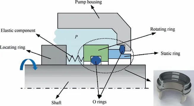
Fig. 1 Schematic of mechanical seals.

The Probability Density Function (PDF) of the USP is dependent on two parameters: α(t ) and β(t ). Both have the functions of μ, σ, and Λ(t ). The Y(t )=USP(t ) can be expressed as Y(t )=USP(α (t )，β(t )).

A predefined threshold for the performance indicator is d,and the failure time T when the threshold is exceeded for the first time is defined as:

(1) Wiener Process

When the USP is a Wiener process with the mean value μΛ(t ) and variance σ2Λ(t ), the following applies:

where α(t )=μΛ(t ) and β(t )=σ2Λ( t ). The PDF of Y(t ) is defined as follows:

The independent increment ΔY(t )=Y(t+Δt)-Y(t ) follows a normal distribution:

where ΔΛ(t )=Λ(t+Δt)-Λ( t ).Therefore,the PDF of ΔY is:

The Cumulative Density Function (CDF) of ΔY is:

The reliability function based on the Wiener process is defined as:

(2) Inverse Gaussian Process

When the USP is an IG process with the mean value μΛ(t )and variance σ2Λ(t ), the following applies:

The independent increment ΔY(t )=Y(t+Δt)-Y(t ) follows an IG distribution:

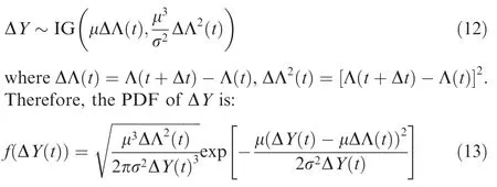
The CDF of ΔY is:

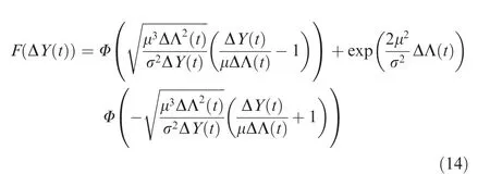
The reliability function based on the IG process is defined as:

(3) Gamma Process

When the USP is a Gamma process with the mean value μΛ(t ) and variance σ2Λ(t ), the following applies:

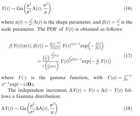
where ΔΛ(t )=Λ(t+Δt)-Λ( t ).Therefore,the PDF of ΔY is:

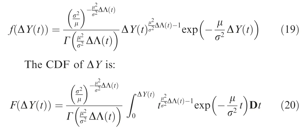
The reliability function based on the Gamma process is defined as:

where γ(·) is the lower incomplete gamma function.

Table 1 shows the relationship between α(t ), β(t ) and μ, σ,Λ(t ). Based on the previous discussion, the marginal distribution of the two performance indicators is obtained and is used as the input data for the copula function.

2.3. Reliability estimation based on the bivariate copula model

A copula function is an effective method to combine the multivariate probability distribution of different performance indicators into a combined distribution. Based on Sklar’s theory44, a bivariate copula function can be defined as:

where θ represents the strength of dependence between two variables.F1(x1)and F2(x2)are two uniformly distributed random variables with the interval [0，1 ]. In the following discussion, u and v denote F1(x1) and F2(x2), respectively. The density of a copula function is defined as:

The density function is expressed as:

Table 2 shows several copula functions that are used in this study. All these seven copulas can represent the main familied of copula function, and they commonly applied in reliability estimation for mechanical components. The density function of the copula function is shown in Appendix A.

Kendall’s tau is a non-parametric measure of the dependence between two variables in copula functions. It is defined as the probability of concordance minus the probability of discordance of two independent vectors. In a copula function,Kendall’s tau is calculated as:

Table 1 Parameter definition for the three stochastic models.

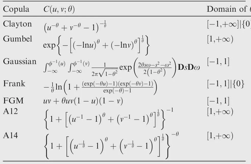
Table 2 Definition and parameter domain of different copula functions.

Table 3 shows Kendall’s tau values and the corresponding domains of the different copula functions.

Let d1, d2denote the threshold for the performance indicators Y1(t ), Y2(t ), respectively. The reliability function is expressed as:

If two performance indicators are independent,Eq.(26)can also be defined as:

If two performance indicators are dependent, Eq. (26) can be obtained through the Monte Carlo method45.

The mean time to failure (MTTF) is expressed as:

2.4. Statistical inference

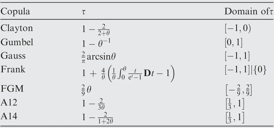
Table 3 Kendall’s tau and its domain.

The degradation model of the test samples considering the univariate degradation model uncertainty and the dependence between the two dependent performance indicators is defined as:

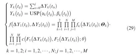
where Θk= (μk，σk，qk) represents the unknown parameters in the unified degradation model of each performance indicator,and θ represents the dependence parameter in the copula function.

All the unknown parameters in Eq. (29) need to be estimated, and a MA method is used to determine the optimal model and reliability function. The log-likelihood function based on the degradation data D and the degradation model is derived as:

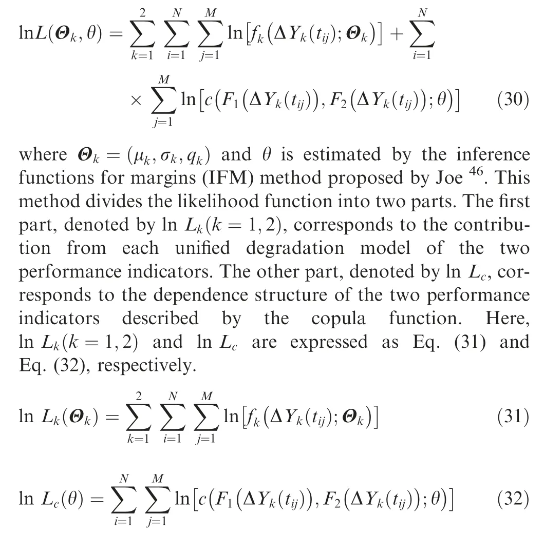
where ln Lk(Θk) are obtained using Eqs. (33), (34), and (35),assuming that the models M1, M2, and M3denote the Wiener process, IG process, and Gamma process, respectively.

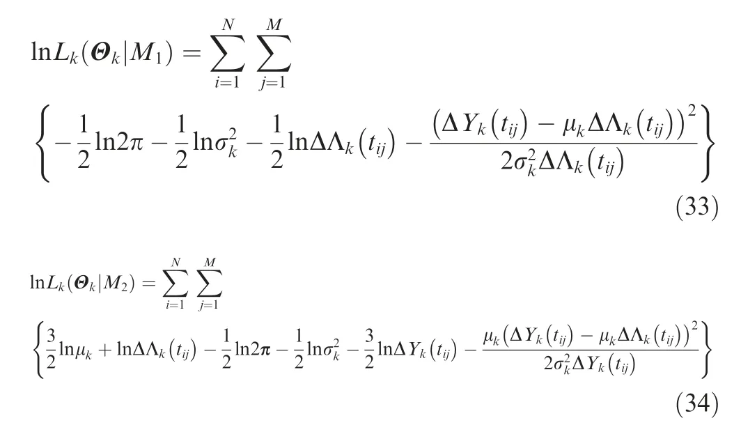
The IFM method estimates the parameters in two stages.The MCMC method is utilized to estimate the unknown parameters in each stage. A Markov chain with a stationary distribution as the prior distribution is used to obtain the samples of the posterior distribution by observing the chain after a number of steps. The closer distribution to posterior distribution of unknown parameter can be obtained. Various algorithms exist for constructing the chains, including Metropolis-Hastings algorithm and Gibbs sampling algorithm.The estimation process is conducted in the software Open-BUGS by using Gibbs sampling algorithm. In the first stage,Θk= (μk，σk，qk) in the USP degradation model is estimated based on the log-likelihood lnLk(Θk). In the second stage, θ in the copula function is estimated based on the loglikelihood lnLc(θ ). Non-informative priors for the parameters are selected in our study.The posterior probability of Θkand θ are expressed as Eq. (36) and Eq. (37), respectively.

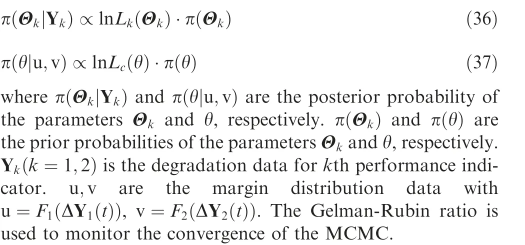
After all the unknown parameters have been estimated,the reliability function and MTTF are obtained.

3. Bayesian model average method

It is possible to identify an optimal model since we have obtained the three stochastic process degradation models describing the degradation process of each performance indicator and the copula function set that includes seven copulas describing the dependence between the two performance indicators.The BMA method,which integrates prior knowledge of the model and the log-likelihood function of the degradation data, is used to choose the probable model37. The BMA method is well suited for dealing with the uncertainties of degradation models and has been applied in many fields.

3.1. Bayesian model average

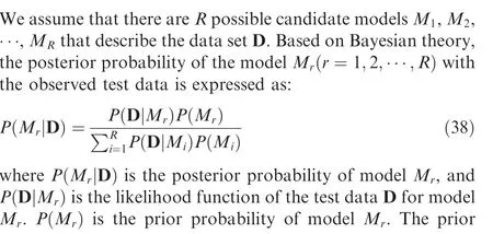
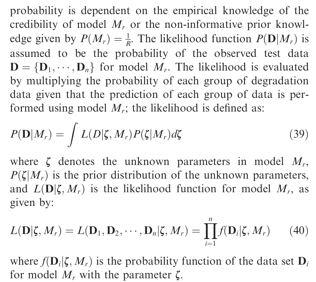
The posterior probability of model Mr, which is also the probability of selecting model Mr, is proportional to the prior model probability and model likelihood based on the discussion above; we assume that:

All plausible models should be taken into account, and their weight can be calculated by Eq. (41). Then, the MA method is used to average the weighted model predictions as follows:

where Wris the weight of model Mr. The model with the largest value of Wrshould be selected.

It can be concluded that the BMA method considers the model uncertainty and the parameter uncertainty by integrating model predictions weighted by model probabilities. In the following section, we will show how the MA method is used to select the stochastic process model for each performance indicator and each copula function.

3.2. BMA method for the selection of the stochastic process model

The BMA method is utilized to select the suitable model for each performance indicator and copula function. The integrated function in Eq. (39) cannot be easily computed. Therefore, the MCMC in OpenBUGS is used.

The goal of degradation modeling is to select the model that best captures the degradation process using the available degradation data. The Wiener process, Gamma process, and IG process are commonly used to describe the degradation process, and they are selected as candidate processes in our study.

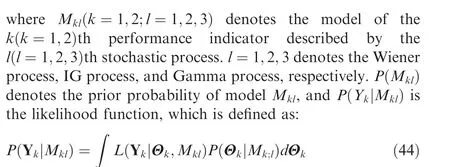
(1) Model Prior Probability P (Mkl)

P(Mkl) is the prior probability or the degree of belief that model Mklis the best approximation to describe the degradation process of the performance indicator. It can be set based on expert knowledge or as non-informative prior knowledge.In our study, non-informative prior knowledge is adopted and is expressed as:

(2) Unknown Parameter Estimation

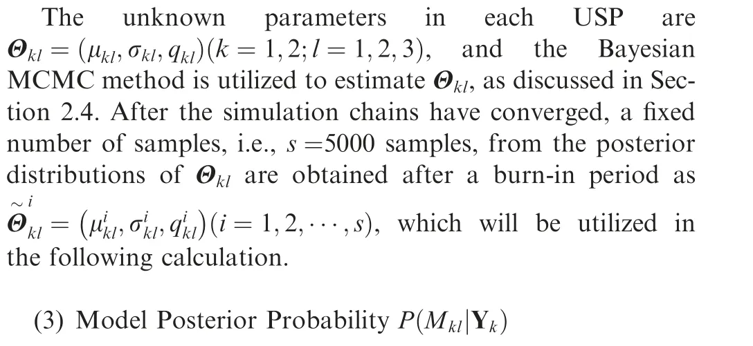
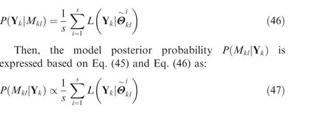
The approximation function in Eq. (46) is substituted into the integrated likelihood function in Eq.(44)by using the samplesfrom the posterior distribution of the unknown parameters37:

(4) Model Average

We define Qklbased on Eq. (41) and Eq. (47) as:

The weight Wklfor model Mklbased on the BMA theory and Eq. (42) is expressed as:

The corresponding USP with the highest weight, i.e., the largest value of Wkl,is the optimal degradation model for each performance indicator.

3.3. BMA copula selection

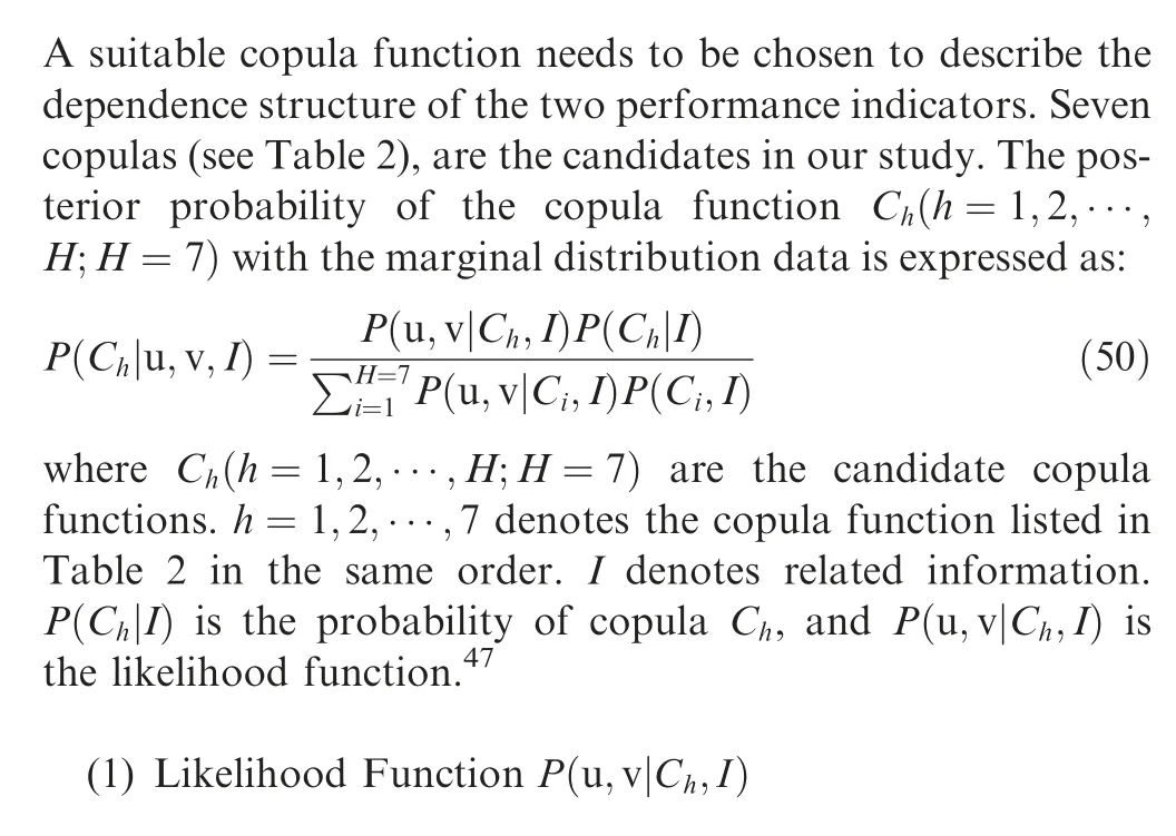
As discussed in Section 2.3, Kendall’ s τ is in one-to-one correspondence with θ, and the value range is always limited.Therefore, with Kendall’s τ, the posterior probability P(Ch|u，v，I) is expressed as:

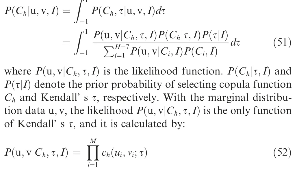
where ch(ui，vi;τ) is the density of the copula function Ch, and M is the number of data points.

(2) Model Prior Probability P (Ch|τ，I) andP (τ|I )

The prior knowledge in Eq. (51) includes the prior knowledge of τ(P(τ|I ))and the prior knowledge of the copula function (P(Ch|τ，I)). Thus, we divide the additional information I into two parts: (i) Information I1on the prior knowledge of Kendall’s τ; (ii) Information I2on the prior knowledge of the copula function Ch.

(i) P (τ|I1):The prior knowledge of τ is the additional prior knowledge of the relationship between the two performance indicators. τ belongs to the set Ψ and each outcome of τ ∈Ψ is equally likely. No additional information is available in our study; therefore, Ψ is assumed to be [-1，1].

where λ(Ψ ) denotes the Lebesgue measure, which is the width of the interval spanned by Ψ.

(ii) P (Ch|τ，I2): For a given τ, all copula function families satisfying τ ∈Ωhare equally probable.Ωhis the domain of τ for the hth copula Ch.

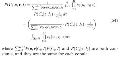
From the discussion above, Eq.(51)can be transformed as follows:

(3) Model Average

We assume that:

The weight Wchfor each copula function Chis expressed as:

3.4. Selection of the modified degradation model

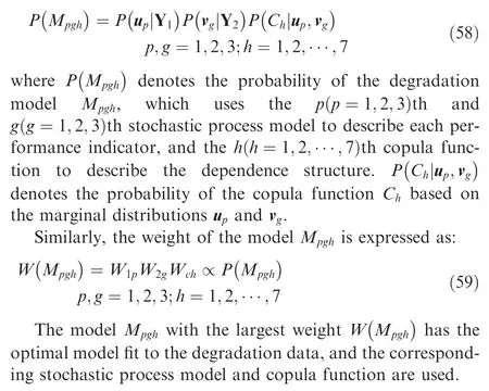
In Section 3.2 and Section 3.3, the uncertainties regarding the stochastic model selection and copula function selection have been addressed. For a group of given degradation data, the combination of the best stochastic model for each performance indicator and the copula function that best describes the dependence structure might not be the best degradation model.The marginal distribution data of each performance indicator are the input data for the copula function, and they could affect the selection of the copula functions. Therefore, it is advisable to consider both aspects simultaneously and choose a suitable degradation model.

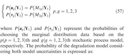
The selections of the marginal distribution and the copula function are independent selections. It is reasonable to assume that the probability of choosing the marginal distribution data for each performance indicator is the same as the probability of choosing the corresponding stochastic model, i.e.:

4. Simulation study

4.1. Case I: Accuracy of the proposed algorithm

A simulation study is conducted to validate the accuracy of the proposed model selection method.We assume that the performance indicator Y1(t )follows an IG process with the parameters μ1=1.94,σ1=0.3534,and q1=1.36,and Y2(t )follows a Gamma process with the parameters μ2=7.46,σ1=1.04,and q1=1.45.The dependent relationship between Y1(t )and Y2(t )is described by the Gaussian copula with the parameter θ=0.9834. The sample size N is 4, and the number of measurements M is 50. The failure thresholds for the two performance indicators are d1=2.5 and d2=15, respectively. The time interval is assumed to be Δt=0.02. The Monte Carlo method is used to generate random degradation data. The degradation path is shown in Fig. 2.

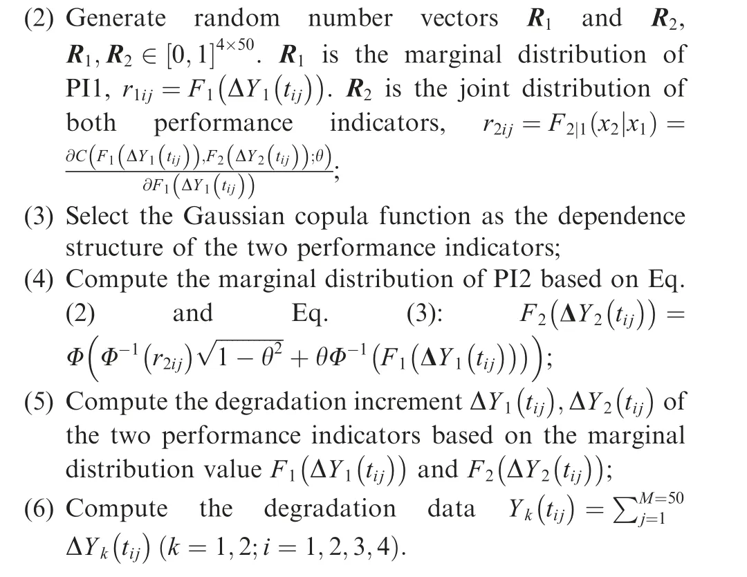
The generating process for each performance indicator is as follows48:

(1) Select the IG process and Gamma process as degradation models for the performance indicator 1 (PI1) and performance indicator 2 (PI2), respectively;

The Wiener process, IG process, and Gamma process are utilized to fit the degradation data of PI1 and PI2,respectively.The estimation results are shown in Table 4. Standard errors and confidence intervals are shown in the Appendix B. The posterior distribution and the Brooks-Gelman-Rubin (BGR)convergence results for each parameter of the IG process of PI1 and each parameter of the Gamma process of PI2 are shown as examples in Fig. 3.

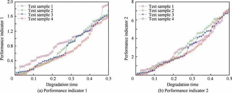
Fig. 2 Degradation path of performance indicators.

Table 4 Parameter estimation results.

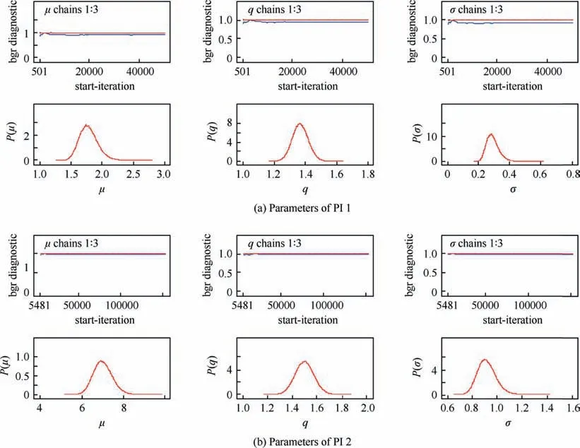
Fig. 3 Posterior distribution and BGR results of parameters of PI1 & PI2.

All the degradation increments of the two performance indicators are positive;therefore,the three stochastic processes are suitable to describe the degradation process. We assume that the prior probability of the model P( Mkl)=(k=1，2;l=1，2，3). Based on Eq. (46) and the estimation results,5000 samples from converged estimation samples are used in the subsequent calculation. The weights of the stochastic processes for each performance indicator are shown in Fig. 4.

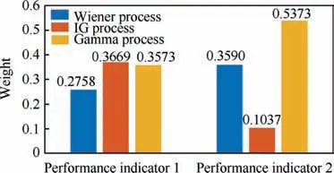
Fig. 4 Weights of stochastic processes of PI1 & PI2.

Fig. 5 shows the scatterplots of the marginal distribution for different stochastic model combinations for PI1 & PI2.Fig. 5(a) shows the comparison of the IG-Gamma and the Gamma-Gamma processes. Similarly, Fig. 5 (b) shows the comparison of the IG-Gamma and the Wiener-Wiener processes.Fig.4 shows that the weights are highest for the IG process for PI1 and for the Gamma process for PI2, indicating that these are the best models to describe PI1 and PI2,respectively. The BMA selection result is the same as the predefined stochastic process for PI1 and PI2.It should be noted that for PI1,the weights are similar for the IG process and the Gamma process.Therefore,it is likely that both the IG process and the Gamma process provide a good fit for the degradation data for PI1. However, differences in the marginal distribution are observed in Fig. 5 (a). The Gamma-Gamma values (red dots)are slightly higher than the IG-Gamma values(blue dots).The selection of the stochastic model for PI1 affects the marginal distribution. For PI2, the weights of the IG process and Gamma process are quite different, and the weight of the Wiener process is larger than that of the IG process.Although the IG process and Gamma process both describe monotonic degradation processes, they do not provide a good fit of the degradation data of PI2 in this study. Although the Wiener process is used to describe non-monotonic degradation processes, it can also be used to describe monotonic degradation processes, and sometimes might be better than the IG process or Gamma process. As shown in Fig. 5 (b), the lowest values for the Wiener-Wiener processes are around (0.2, 0.2), and those of the IG-Gamma processes are around(0,0).This result indicates that different model selections will affect the dependence of the degradation data and affect the copula function selection.

The estimated parameters are utilized to compute the marginal distributions of the two performance indicators of each stochastic process and also as input into the copula functions.For each copula function in the copula set,the prior probability is the same, and the prior probability of τ, P(τ|I ), is also assumed to be the same. The weights of the copula function for different combinations of the stochastic processes for each performance indicator are shown in Table 5 (Eqs. (54)-(56)).The degradation model weights are shown in Table 6. The results show the largest copula function weights of each combination of PI1 and PI2 and the eight largest weights among the 54 combinations.

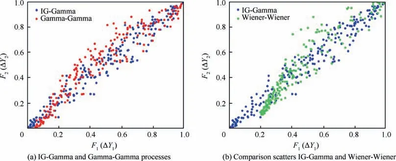
Fig. 5 Scatterplots of marginal distribution for different stochastic model combinations for PI1 & PI2.

Table 5 Weights of copula function for different combinations of stochastic processes.

Table 6 Weight ranking.

Table 6 shows that the largest weight is obtained by using the IG process for PI1 and the Gamma process for PI2 and the dependence relationship described by the Gaussian copula function. The second-largest model weight is obtained when both performance indicators are described by the Gamma process,and the dependence relationship is described by the Gaussian copula. However, there is model uncertainty. The results of the weights calculated by the BMA method are identical to that of the predefined selection.

A reliability estimation is also conducted. Fig. 6 shows six different cases ranging from the 1st to 6th and corresponding to the list in Table 6.The right graph in Fig.6 is a partial magnification of the reliability estimation curve from 1.1 to 1.5 h.It is observed that the reliability curves are substantially different for the six cases. The solid red line denotes PI1 described by the IG process, PI2 described by the Gamma process,and the dependence relationship described by the Gaussian copula function (IG-Gamma-Gaussian combination). The Gamma-Wiener-Gaussian curve is lower than the IGGamma-Gaussian curve.The other four types of combinations are all higher than the IG-Gamma-Gaussian combination.Both the reliability estimation plots and the MTTF results show the errors contributing to model uncertainty. It is necessary to choose an accurate degradation model to describe the degradation process.

Fig. 6 Reliability estimation results of stochastic processes and copula function.

Table 7 Comparison of initial and estimated parameters.

The parameters in the Gaussian copula are also estimated by the Bayesian MCMC method. Table 7 compares the initial and estimated parameters. Regardless of the model selection and parameter estimation, the model selection based on the BMA method is the same as the initial assumption.The sample size (N=10), the number of measurements (M=100), and the relative errors are listed in Table 7.The parameter estimation results have higher accuracy when the sample size and number of measurements are large.Fig.7 shows the reliability estimation results of the three cases,and Table 8 compares the MTTF results for different sample sizes and number of measurements. It is observed that more test samples and more measurements result in more accurate reliability estimation results.The applications and assumptions for this data can be found in Ref.[21].The degradation paths for Crack A and Crack B are displayed in Fig.8.The degradation process of Crack B is not strictly monotonic; therefore, it can only be described by the Wiener process. Crack A can be described by the Wiener process, Gamma process, or IG process. The dependent relationship is described by seven copulas, as shown in Table 2.

Table 8 Comparison of MTTF for different sample sizes and number of measurements.

4.2. Case II: A fatigue crack study

The proposed model is used to analyze fatigue crack data from Ref. [49]. Crack A and Crack B are assumed to be dependent.

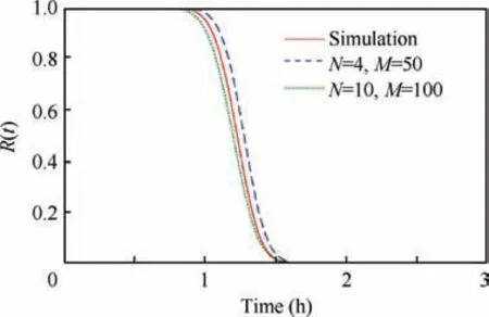
Fig. 7 Reliability estimation results for different sample sizes and number of measurements.

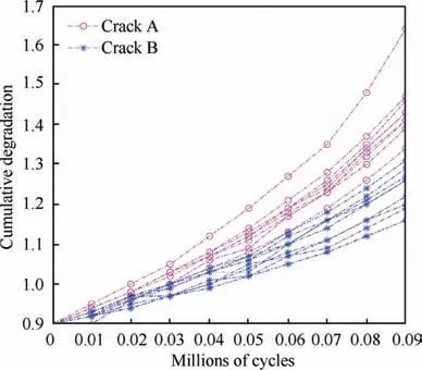
Fig. 8 Degradation paths for Crack A and Crack B.

Table 9 Weights of the models for stochastic processes of Crack A & Crack B.

The selection process is the same as described in Section II and Section III, and the BMA selection results are shown in Table 9 and Table 10, respectively. For Crack A, the Gamma process is the best choice,and the Wiener process has the lowest weight.Regardless of the stochastic process of Crack A,the Frank copula is the most suitable function to describe the dependence relationship between Crack A and Crack B. The selection result is the same as the AIC selection result in Ref.[21].Table 11 shows the weight ranking of the different model combinations. The Wiener process for Crack A and Crack B with the Frank copula has the highest weight, and this combination is the most suitable choice for the degradation model.This result indicates that although the Gamma process is the best selection for Crack A, the weight for the combination of the Gamma process for Crack A,the Wiener process for Crack B,and the Frank copula is lower than that of the Wiener process for Crack A and Crack B with the Frank copula. The stochastic process model uncertainty and the copula uncertainty should be considered simultaneously.

5. Experimental validation

5.1. Introduction to experiment

A degradation test of mechanical seals was conducted to monitor the two performance indicators (leakage rate and friction force) of the mechanical seals, as shown in Fig. 9. The test rig consisted of four parts, including a force adjustment device,test chamber, bearing box, and electro-drive system. Two mechanical seals were installed symmetrically in the test chamber to prevent an axial force due to an increase in the hydraulic pressure. The bearing box was used to avoid axial displacement and runout. The friction of the mechanical seals was measured. The force adjustment device was placed at the tail of the seal, and on-line detection was performed using a pressure sensor. The leakage rate was determined by placing a measurement cup under the test chamber.

Leakage rate and friction force measurements were collected to monitor the degradation process of the test seals.After being conditioned by a signal conditioning module, the signals were collected by a data collection system. The data collection and processing software was programmed in theNational Instruments LabWindows CVI®,and data collection was automatically performed every four hours.For the friction force and contact temperature signal, the sample rate was 1000 Hz, and each collection lasted 20 s. The failure of each seal was manually assessed by the test operators based on the friction force, temperature, and leakage. Once a seal had failed, it was removed from the test rig. A new seal was then installed, and the test was resumed. The operating conditions of the test are provided in Table 12.

Table 11 Weight ranking.

5.2. Model selection using the model average method

The degradation data of the three test seals were used to conduct the reliability estimation. Fig. 10 shows the degradation paths of the test seals from 450 h to 1000 h. Since no leakage occurred from 0 to 450 h for all test seals,the degradation data during this time were not considered.

The degradation increment data of the friction torque were transformed into absolute values. All the degradation data of the two performance indicators were normalized to conduct unknown parameter estimation and reliability estimation.

The degradation increments of both performance indicators are positive. The three stochastic models are suitable to fit the data of the two performance indicators.The unknown parameter estimation results are shown in Table 13. Standard errors and confidence intervals are shown in the Appendix C. The BMA model selection results are shown in Fig.11.The IG process has the highest weight for both leakage rate and friction torque. The weights of the three stochastic models are similar for the leakage rate. For the friction force, the weights of the IG process and Gamma process are similar, and that of the Wiener process is the lowest.Fig.12 shows the posterior distributions and BGR convergence results for the two performance indicators described by the IG process.

Table 14 shows the weights of the copula function for the nine stochastic model combinations of the two performance indicators. Fig. 13 shows the bar chart of the same data. The weights of the copula functions for the leakage rate and friction torque described by the IG process is shown in Fig. 13(a). The Gaussian copula has the highest weight, and the Frank copula has the second-highest weight. The result indicates that the Gaussian copula is the most suitable selection for the IG-IG combination. The weights of the copulafunctions for the leakage rate described by the Wiener process and the friction torque described by the Gamma process are shown in Fig. 13 (b). In this case, the Gaussian Copula also has the highest weight, and the value is higher than that of the IG-IG combination.

Table 10 Weights of copula function for different combinations of stochastic processes.

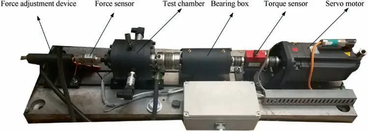
Fig. 9 Degradation test rig used for degradation test of mechanical seals.

Table 12 Operating conditions of degradation test.

Table 15 shows the nine largest weights of the model out of sixty-three combinations. The largest weight is observed for the combination of the leakage rate described by the Wiener process, the friction torque described by the Gamma process,and the dependence described by the Gaussian copula(Wiener-Gamma-Gaussian). Therefore, this combination is most suitable to describe the degradation process of mechanical seals. The IG-IG-Gaussian model, which is the model based on the most suitable stochastic model for each performance indicator, has the fifth-largest weight. The model

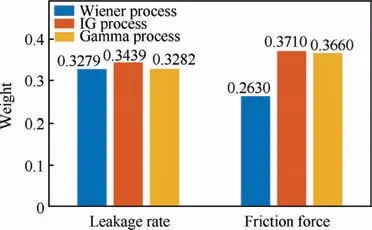
Fig. 11 Weights of stochastic processes of leakage rate and friction torque.

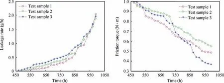
Fig. 10 Degradation path of leakage rate and friction torque.

Table 13 Parameter estimation results.

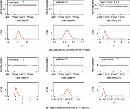
Fig. 12 Posterior distribution and BGR results of parameters for leakage rate and friction torque.

Table 14 Weights of copula function for different combinations of stochastic processes.

ranking results indicate that the weight of the stochastic model and the copula function should be considered simultaneously to obtain the optimum degradation model and accurate reliability estimation. The model based on the suitable stochastic model for each performance indicator might not be the best model to describe the overall degradation process.

5.3. Reliability estimation & model uncertainty analysis

The reliability estimation results of the mechanical seals under the given working conditions are shown in Fig. 14. Six different models are considered, including the Wiener-Gamma-Gaussian, Gamma-Gamma-Gaussian, Wiener-Wiener-Gaussian, IG-IG-Gaussian, leakage rate, friction torque, only and considering independent relationship between leakage rate and friction torque. The dashed green line (friction force) is much higher than the other models, and the dashed cyan line(Wiener-Wiener-Gaussian model) has the lowest values. The partial magnification of the curves of the other five models from 750 h to 850 h is shown on the right in Fig. 14. The reliability curves are quite different due to the model uncertainty issue in model selection. The MTTF and relative errors are shown in Table 16. The true lifetime is obtained from the degradation test after the mechanical seal has failed. The Wiener-Gamma-Gaussian model has the lowest relative error,indicating that this combination is the most suitable model to describe the degradation process. The friction force has the highest relative error, demonstrating that the use of only one performance indicator does not provide accurate lifetime estimation.

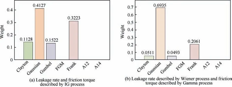
Fig. 13 Weights of copula function.

Table 15 Weight ranking.

Fig. 14 Reliability estimation results of mechanical seals.

Fig.15 shows the joint PDF of the leakage rate and friction torque based on the Eq.(24).The different models provide different PDF distributions at the given degradation time. The distribution of the Wiener-Gamma-Gaussian model (solid red line)is much narrower than that of the other models,indicating that the Wiener-Gamma-Gaussian model has higher accuracy than the other models.

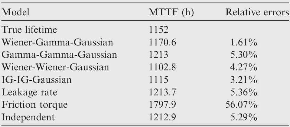
Table 16 Comparisons of MTTF for different sample sizes and number of measurements.

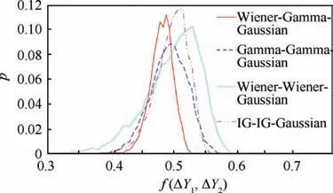
Fig. 15 Joint PDF of two performance indicators at 600 h.

6. Conclusions

A reliability estimation model for mechanical seals was established based on the failure mechanism and using bivariate dependence analysis.The friction torque and leakage rate were used as performance indicators of the degradation process of the seals. The degradation was described by the Wiener process, Gamma process, and IG process, and the dependence between the performance indicators was described by different types of copula functions. The BMA method was utilized to analyze model uncertainty in the stochastic process degradation models of the performance indicators and the dependence between the two performance indicators. The degradation model was selected by considering the weights of the stochastic process models and the weights of the copula function simultaneously. The unknown parameters in the degradation model were estimated by the Bayesian MCMC method. A degradation test of the mechanical seals was conducted to validate the proposed model. The validation results and model uncertainty analysis of the reliability estimation demonstrate the excellent performance of the proposed model. In addition, a numerical simulation study and a fatigue crack study also verified the accuracy of the degradation model. In the future, we will extend this work by conducting an ADT and considering model uncertainty for other mechanical and electrical components. The prior probability of potential models can also be obtained by expert knowledge or engineering experience.

Declaration of Competing Interest

The authors declare that they have no known competing financial interests or personal relationships that could have appeared to influence the work reported in this paper.

Acknowledgements

This study was supported by the National Natural Science Foundation of China (Nos. 51875015, 51620105010).

Appendix A

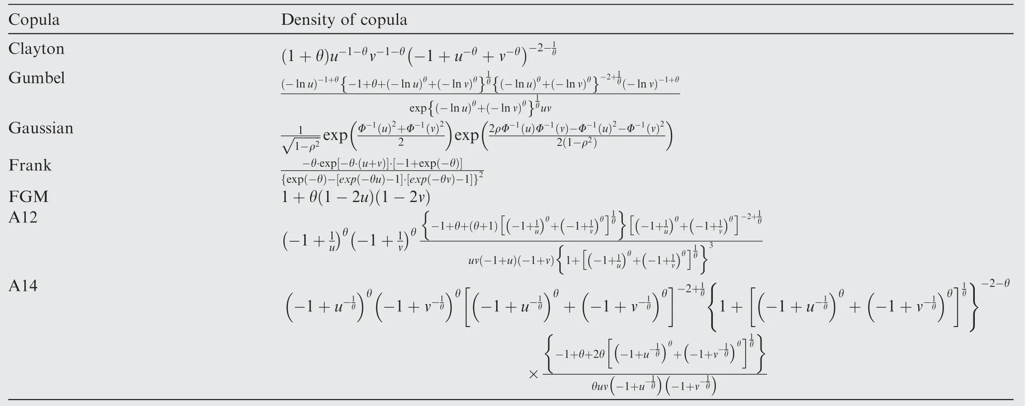
Table A1 Density function of copula used in this study.

Table A2 Mean value, standard errors (Sd) and 95% confidence intervals(CI) for parameters in Table 4.

Table A3 Mean value, standard errors (Sd) and 95% confidence intervals(CI) for parameters in Table 13.