Identification of key factors affecting the failure of aviation piston engine turbochargers based on an improved correspondence analysis-polar anglebased classification

Mengyo BAO, Shuiting DING, Guo LI,*

a Civil Aviation Management Institute of China, Beijing 100102, China

b Aircraft/Engine Integrated System Safety Beijing Key Laboratory, Beihang University, Beijing 100083, China

KEYWORDS Failure-inducing factors;Improved correspondence analysis;Polar angle;Turbochargers;Whole-machine system model

Abstract Turbocharging is an efficient approach for addressing power reduction and oil consumption increase in aviation piston engines during high-altitude flights.However,a turbocharger significantly increases the complexity of a power system,and its considerably complex matching relation with the engine results in a coupling of failure modes.Conventional analytical methods are hard to identify failure-inducing factors. Consequently, safety issues are becoming increasingly prominent.This study focuses on methods for identifying failure-inducing factors. A whole-machine system model is established and validated through experimentation. The response surface method is employed to further abstract the system simulation model to a surrogate model (average error: ～3%)in order to reduce the computational cost while ensuring accuracy.On this basis,an improved Correspondence Analysis (CA)-Polar Angle (PA)-based Classification (PAC) is proposed to identify the key factors affecting the failure mode of turbochargers.This identification method is based on the row profile coordinates G varying with the numerical deviations of the key factors, and is capable of effectively identifying the key factors affecting the failure. In a validation example, this method identifies the diameter of the exhaust valve (e2) as the primary factor affecting the safety margin for each work boundary.

1. Introduction

Aviation piston engines are an important choice for power systems in aircraft and thus used in the majority of aircraft.1,2Turbocharging is an efficient approach for addressing the power reduction and oil consumption increase during highaltitude flights.However,a turbocharger significantly increases the complexity of a power system. Safety issues related to turbochargers are becoming increasingly prominent.According to a survey report published by the U.S.National Transportation Safety Board (NTSB), 111 aircraft accidents caused by turbochargers occurred from 1988 to 2008, leading to 29 deaths and 38 injuries.3-5Most of these accidents were attributed to engine power failure caused by turbocharger malfunctions.Therefore, the U.S. NTSB has recommended that the U.S.Federal Aviation Administration (FAA) pay particular attention to turbocharger-induced power reduction and loss in aviation piston engines.3Additionally, the U.S. NTSB has also stated that ‘‘due to the lack of measures for preventing turbocharger failure in previous engineering practice,it is recommended that the factors affecting turbocharger failure and the potential factors causing turbocharger failure be identified to prevent turbocharger failure”.6Therefore, how to identify the key failure-affecting factors during actual operation is vital for accurately formulating failure risk control strategies for operation and maintenance,as well as for ensuring general aviation flight safety.

Generally, the failure of a turbocharger is attributed to its inherent lag and positive feedback resulting from its pneumatic connection with an engine.(A)Lag refers to the inability of the compressor in the turbocharger to respond when there is a change in the engine conditions. (B) Positive feedback refers to the following behaviours:when the engine load is low,a relatively low exhaust energy results in an insufficient working capacity of the turbine, which further worsens the intake air conditions for the engine, or even shuts down the engine altogether; when the engine load is high, a relatively high exhaust energy results in an increase in the work done by the turbine and its rotational speed, which further increases the intake air pressure and can easily cause the engine to race and knock.Therefore, the turbocharger and the engine exhibit a strong,complex matching relation and closed-loop characteristics,resulting in a coupling of failure modes.7,8Consequently, it is difficult to use conventional analytical methods to decompose and identify failure modes that occur during operation and determine their affecting factors.For example,these methods are unable to perform a fault tree analysis in the system safety analysis and address ‘‘closed-loop events” in complex systems.9During actual operation and maintenance, it is even more difficult to use these methods to accurately formulate and implement targeted failure risk (or safety) control strategies. Additionally, these methods are unable to fundamentally address turbocharger failure or ensure operational safety.

To overcome the limitations of conventional analytical methods in solving complex coupled engineering problems,model-based failure-causing factor analytical methods have been developed in recent years.10,11In model-based failurecausing factor analysis, a complex system model specific to a study object is introduced into the failure mode analysis. In other words, an established model is used to test a system through a simulation at each stage of the failure mode analysis in order to determine whether the system can operate according to functional requirements. During this process, the same model is used in the failure mode analysis and the system examination. This will reflect the matching and coupling between systems and then effectively identify the failure mode.The Advisory Circular 20-115C issued by the U.S. FAA has officially confirmed that the DO-331 model-based analysis and testing can be used in an airworthiness certification of airborne systems and equipment development.12

Hence,this study examines a certain aviation piston engine and its two-stage turbocharging system. Based on an established system model, an improved Correspondence Analysis(CA) method is proposed, which is combined with Polar Angle-based Classification (PAC) to identify key factors affecting the failure mode of the turbocharger. The results of this study will directly support the identification of affecting factors and potential factors causing the failure of turbocharging systems for aviation piston engines during actual operation. Additionally, the results of this study will facilitate the formulation of targeted preventative measures. This article consists of six sections. Section 2 describes the mechanisms by which the improved CA and PAC are applied to turbocharger failure. Section 3 introduces an established wholemachine system model for a typical turbocharged aviation piston engine and examines its accuracy. Section 4 presents the identification of the key factors affecting the failure of the turbocharging system. Section 5 discusses identification analysis results. Section 6 summarizes main conclusions.

2. Analysis of application mechanisms of an improved CA and PAC

2.1. Analysis of CA mechanism

CA,also referred to as correlation analysis or R-Q factor analysis, is a new multivariate dependent variable statistical technique developed in recent years to analyse dependent variables.13Because CA was developed based on R and Q factor analyses, this method essentially uses a dimensionality reduction approach to simplify the data structure.14-16Generally, the entire process of CA consists of two parts, namely, a contingency table and a two-dimensional (2D) plot. The contingency table is a 2D table composed of rows and columns.Each row represents one attribute of the objects and is arranged in a proper order, while each column represents different objects and is composed of a sample set. Additionally,each row or column of the contingency table can be represented by a point in the 2D plot to more visually describe the interrelations between the states of an attribute variable and between the attribute variables themselves.17-19See Appendix A for the basic principle and application process of CA.

2.2. Proposal of an improved CA and an analysis of its mechanism

The original plan was to use CA to analyse the key factors affecting the failure of the turbocharging system examined in this study. Specifically, the key influencing factors and work boundary safety margins are treated as sample points (row points) and variable points (column points), respectively. The extent to which each of the key factors affects the turbocharging system is then determined based on the relationship between the key influencing factors (independent variables)and the work boundary safety margins(dependent variables).8However, there are several issues when directly introducing CA:

(1) The results of CA depend on the influencing factors and work boundaries. Therefore, to obtain the complete influencing factor and work boundary information from the original data,it is necessary to maximally sample the system model. This, however, will result in a high computational cost.

(2) CA requires that the variable points in the original data have the same dimensions(or be dimensionless)and that the error caused by the difference in the order of magnitude between the influencing factors be minimized.20When analysing a turbocharging system, selecting work boundary points such as the turbine inlet temperature and rotor speed as influencing factors will cause some problems.Firstly,there is a difference in the dimensions between these factors. Secondly, there is also a significant difference in the extent of data variation between these factors. Therefore, direct CA is impossible.

In view of the aforementioned problems, the following improvement measures (i.e., improved CA) are proposed:

(1) The response surface method is thus employed to represent each work boundary outputted by the system model with a key influencing factor function, i.e., to construct an equivalent surrogate model to replace the actual model.21-24On this basis, the surrogate model is randomly sampled to generate the basic data requirement for CA.This measure significantly reduces the computational time required for sampling and improves the analytical efficiency.

(2) Prior to further analysis of the failure model and the relationships between the key influencing factors, the data outputted by the surrogate model is subjected to type normalization, i.e., the work boundaries are converted to work boundary safety margins.

2.3. Analysis of key influencing factor identification mechanism based on improved CA and PAC

During an actual development process, how to determine the factors affecting the failure of a turbocharging system based on the observed failure data is the core of the key influencing factor identification. In essence, the process of identifying the key influencing factors based on failure data is the reverse of CA. Thus, in the basis of the improved CA, an identification method based on the variation of the row profile coordinates G and the classification of polar angles with the numerical deviation of the key influencing factors is proposed. Here,the use of PAC mainly involves three steps,namely,PA calculation, cluster centroid determination, and cluster validation.

2.3.1. PA calculation

In most actual cases, when m is set to 2 for the R-Q factor matrix in Appendix A, a point plot can be produced on the same 2D plane based on the row profile coordinates G and the column profile coordinates F.16Based on the Euclidean distances between the corresponding points in the 2D scatter plot,the relationships between the correlated row and column points can also be analysed. However, the row profile coordinates G and the column profile coordinates F will vary with the numerical deviation of the key influencing factors. These variations can be measured based on changes in the relative distance and direction in the 2D scatter plot.

Generally, it is more effective to identify the key factors based on a change of the direction than a change of the distance.14Thus, the change in the direction of the row points or column points in the 2D scatter plot can be measured using the PA.Fig.1 shows the PAs of 2D scatter points used in CA.

(1) The following equation shows the expression of the PA θiof a row point:

where Gi,1and Gi,2are the first and second vectors of the row profile coordinates G, respectively.

(2) Similarly, the following equation shows the expression of the PA φiof a column point:

where Fj,1and Fj,2are the first and second vectors of the column profile coordinates F, respectively.

The key influencing factors can be identified by observing changes in the distance and the PA of a sample point set composed of row points after a numerical deviation of a certain influencing factor occurs. The PA measurement is illustrated in Fig. 2, which shows a schematic diagram demonstrating the variation in the row profile coordinates G with the numerical deviations of the key influencing factors.

(1) As shown in Fig.2,when there is a change in the numerical values of the influencing factors, the sample point row profile coordinates G will deviate from their original positions.However,factors 1 and 2 cause the row profile coordinates G to deviate in different directions. Additionally, the direction of deviation of the sample point row profile coordinates G that occurs when factors 1 and 2 both deviate from their respective original numerical values also differs from that when either factor 1 or 2 deviates from its original numerical value alone.Thus,it is possible to identify the key influencing factors based on the direction of deviation of the sample point row profile coordinates G.

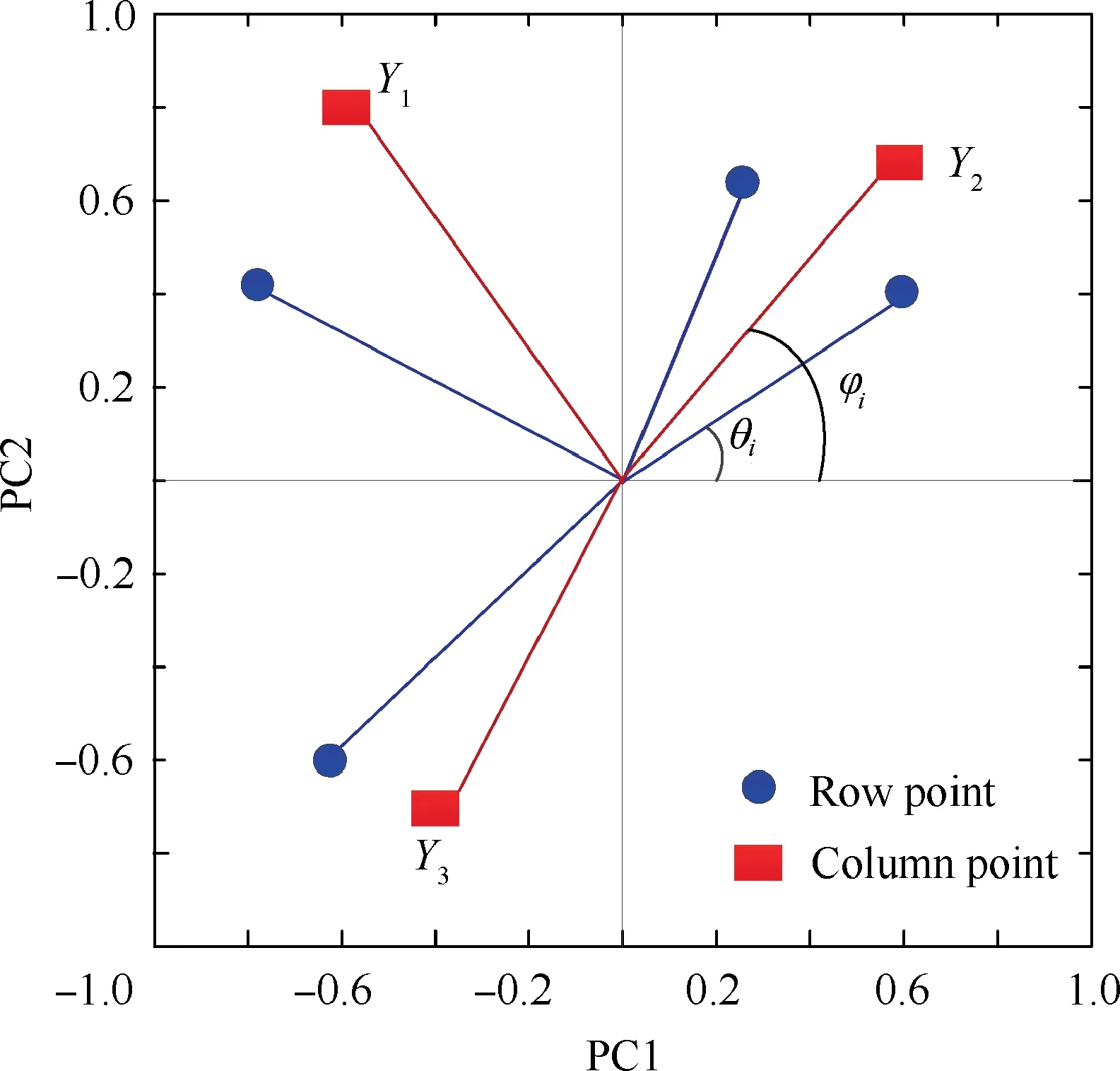
Fig. 1 Distribution of PAs for 2D scatter points in CA.

2.3.2. Cluster centroid determination method

The corresponding cluster and cluster centroid are required to calculate the PA of a sample point cluster. Thus, this section introduces a cluster centroid determination method in detail.For a known cluster centroid (i.e., the central point of the cluster), we begin by assuming K clusters in a biplot for the given dataset. Then, we denote φk(k=1, 2,..., K) to be the cluster centroid of each of these K clusters.Each of the K clusters would be represented by a cluster prototype, θi(i=1,2,..., n) as the characteristic point in each cluster prototype,and Sk(S1∪S2∪...∪SK=X)as the set of characteristic points contained in each cluster prototype.The centroid of each cluster is determined by an optimization procedure.

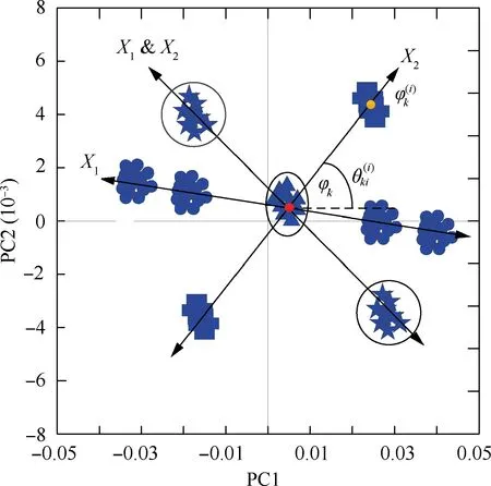
Fig. 2 Deviation of row profile coordinates G with changes in numerical values of key influencing factors when there are a large number of sample points.

Firstly,the angular distance between any two known points(a, b) can be mathematically expressed by the following equation:

Thus, the angular distances between all the characteristic points θiin a cluster prototype and its centroid φkcan form an angular distance matrix. There is a corresponding angular distance matrix for each of the K number of cluster prototypes contained in the set of all the sample point data. Based on these angular distance matrices, a classification label can be defined for the cluster prototypes as

Thus, based on this classification label, the cluster prototypes in the data set can be classified.

Then,based on the classification of the cluster prototypes in the data set, it is necessary to establish objective functions of the intra-cluster data point distance minimization and the inter-cluster data point distance maximization.

(1) The distances between the data points within one cluster

can be defined as follows:

where nkis the total number of data points contained in this cluster. Thus, the total intra-cluster data point distance can be defined as follows:

(2) Similarly, the distances between the data points in two clusters can be defined as follows:

Thus,the objective functions of the intra-cluster data point distance minimization can be expressed by the following equation:

Then, the centroid can be determined based on the objective function of the minimization (J).

2.3.3. Cluster validation

One difficulty in PAC is how to determine the optimum number of clusters for analysis due to the limitations of the cluster classification algorithm.25,26Therefore, it is often necessary to introduce cluster validation to overcome this difficulty.Cluster validation has thus become an important area of cluster classification. Its purpose is to determine whether the number of clusters obtained by the cluster classification algorithm is optimal. Cluster validation generally involves the following four steps:

Step 1. Initialize the parameters of all the clusters but cluster K.

Step 2.Run the cluster algorithm after the user assigns values to the corresponding different parameters of cluster K={2, 3,..., Kmax}.

Step 3. Calculate the validity index (also referred to as the silhouette index) for each obtained cluster.27

Step 4. Select an optimum K value based on the validity index values.

The above steps of cluster validation can be mathematically expressed as follows:

(1) Determine the silhouette width Sij, which can be expressed as follows:

where aiand biare the average distance and the minimum average distance between the ith sample and all the other samples in the jth cluster,respectively.Thus,the value of Sijranges from-1 to 1. Sijof a compact, well-separated cluster tends to be 1. Conversely, Sijof a loose, poorly separated cluster tends to be -1.

(2) Calculate the cluster silhouette value CSjusing the fol

lowing equation:

where m is the number of sample points in the jth cluster.

(3) Determine the global silhouette value GS, which can be expressed as follows:

It is worth noting that GS is the validity index.27The number of clusters can be considered optimal when the validity index reaches the maximum value.

3. Establishment and validation of a turbocharged piston engine system simulation model

The difficulty in analysing the turbocharge failure in a piston engine can be attributed to the complex matching relation between the turbocharger and the engine, as well as the coupling of failure modes.7,8Therefore, it is necessary to firstly establish an entire machine-based system simulation model to accurately reflect the system pattern, thereby laying a foundation for the subsequent analysis of the key failure-affecting factors. In this study, a system simulation model was established based on a Rotax 914 aviation piston engine equipped28with a new two-stage turbocharger.For this new turbocharger as shown in Fig. 3, two-stage compressors have a ‘‘back to back” arrangement with one turbine. This novel scheme enlarges the flow range and allows the engine to operate within the high-efficiency range of the compressors.The details of this two-stage turbocharging system has been given in Refs.29-31The involved indices are as follows: altitude, 10000 m; load,100%; rated rotational speed, 5500 r/min; output power,70.5 kW;total pressure ratio,5.2;average exhaust temperature at the turbine inlet, 1123 K.

Based on the overall design, the two-stage turbocharged engine system was modelled using the GT-Power software(Fig. 4). In this two-stage turbocharged engine system model,a single turbine drives two coaxial compressors connected in series. Additionally, there is an exhaust valve inside the turbine.

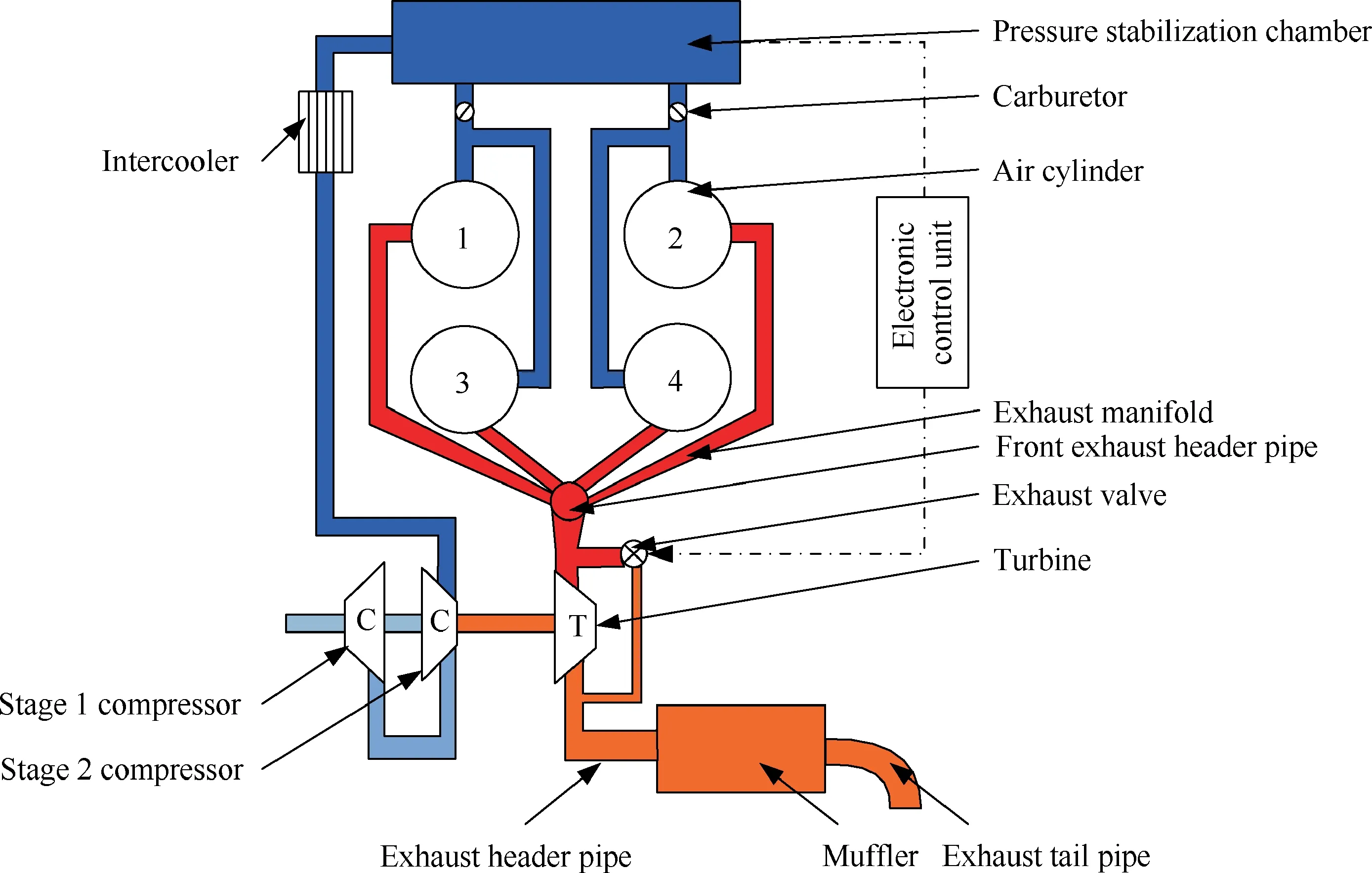
Fig. 3 Schematic diagram of two-stage turbocharging system.

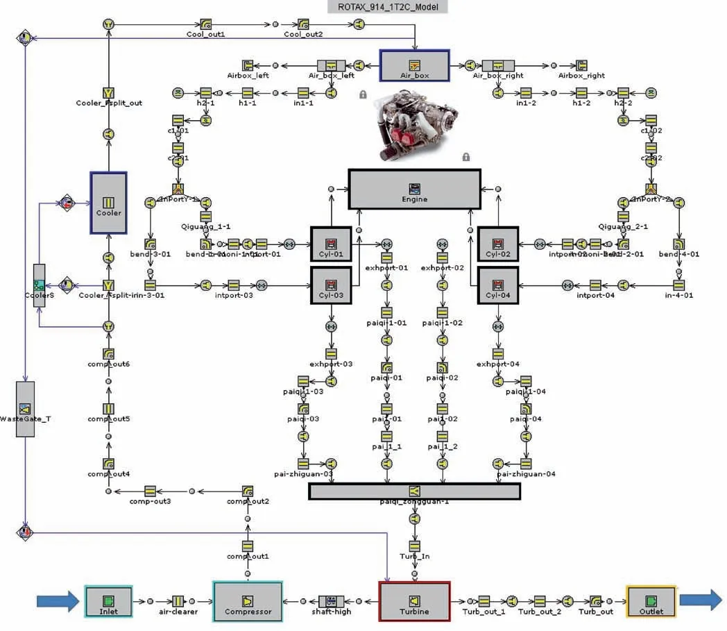
Fig. 4 Schematic diagram of two-stage turbocharged aviation piston engine system model.

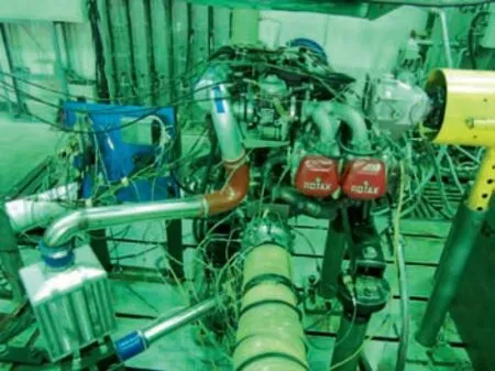
Fig. 5 Experimental two-stage turbocharging system.

To examine the accuracy of the model,results generated by the simulation model were compared with data obtained from a characteristic experiment.This characteristic experiment was conducted on an experimental bench (simulated altitude test facility of piston aeroengines as shown in Fig.5)in the Microengine Laboratory at Beihang University. The experimental system consists of a two-stage compressor system, a turbine,an after-cooler, an air intake pipe, an exhaust pipe, and a transmission control unit. The turbine is coaxial with, and simultaneously drives,the two-stage compressors.The exhaust is ultimately discharged to the atmosphere via the muffler and exhaust tail pipe. In other words, this system has a coaxial structure consisting of two series-connected air compressors driven by one turbine. Additionally, in this design scheme,external air enters the stage 1 compressor and is then compressed.The compressed air then enters the stage 2 compressor and is further compressed. Subsequently, the compressed air enters the pressure stabilization chamber via the intercooler.The engine exhaust enters the turbine via the exhaust pipe and does work in the turbine via expansion. The mass flow of the exhaust used to do work in the turbine via expansion is varied by controlling the opening of the exhaust valve. This allows the actual air intake pressure in the pressure stabilization chamber to be the same as the target pressure, which thereby ensures a safe operation of the engine under various working conditions.

The main advantages of this design scheme are summarized below:

(1) Use of a single-turbine system can increase the exhaust utilization efficiency.

(2) There is no need to consider the turbine flow allocation.Adjustment and control are easy at full-flight altitude.

(3) This design can help reduce the rotational speed of the turbocharger,reduce the number of system components,and increase safety.

(4) The serial connection of compressors increases their flow range, allowing the engine to operate within the highefficiency range of the compressors at full-flight altitude.

(5) Research and development as well as manufacturing are relatively easy.

During the experiment, the ambient temperature and pressure were 20°C and 100.7 kPa, respectively, and the working conditions were built by the simulated altitude test facility of piston aeroengines.Because this paper focuses on the proposed identification method, thus full experiment results at different altitudes are not given, but typical operating points are presented. Calculations were conducted for operating points at rotational speeds of 3000-5500 r/min (intervals of 500 r/min)and 5800 r/min. Figs. 6 and 7 compare simulated and experimental data for changes in the output power and torque of the engine, respectively, when the throttle valve was opened to various extents. Clearly,model-simulated values agreed relatively well with experimental ones within the allowable range.After the throttle valve of the engine was opened over 60%,the differences between the experimental and simulated values of the output power and torque gradually decreased from 6%to less than 3%. Thus, the established simulation model reflects the characteristics of the system relatively well and can be used for subsequent analysis.

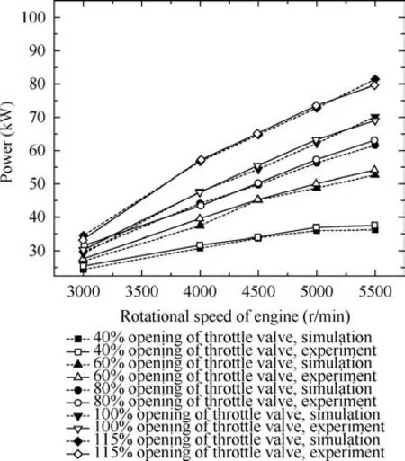
Fig.6 Comparison between simulated and experimental data for output power.

Fig.7 Comparison between simulated and experimental data for torque.

4.Identification of key factors affecting failure of turbocharging system

Based on the mechanism analysis in Section 2, the key factors affecting the failure of the turbocharging system are identified using the following process.

4.1. Surrogate modelling based on response surface method

The response surface method is used to establish a surrogate model to describe the work boundaries corresponding to the safe boundaries during the operation of the system under the complex matching relation between the turbocharging system and the engine. These work boundaries are then represented by a function of the key influencing factors as follows:

where yomis each work boundary that needs to be monitored during the operation of the entire system (i.e., the operating state function of the system),m is the number of work boundaries,n is the number of key influencing factors,and e1,e2,...,enare the key influencing factors. This function can be represented by a linear polynomial containing quadratic cross terms(t0,ti,tii,tijare the coefficient and ε is the error).For each work boundary yom, this function can be expressed as follows:

Then,the response surface method can be further employed to design an experiment on the key influencing factors and estimate the parameters of the response surface model. The function of the response surface model is expressed as follows:

4.2. Data type normalization

Data type conversion is performed for the variable points selected for the turbocharging system.Specifically,the variable point data is normalized to a uniform dimension and order of magnitude, and then CA is conducted.32,33Thus, the index normalization method is employed to convert the work boundary points represented by the variable points in the original matrix X=(xij)n×pto the safety margins for the work boundary points, in order to eliminate the differences in the dimension and order of magnitude. The original matrix X=(xij)n×pis manipulated based on the following transformation relation:

where xmaxand xminare the upper and lower bounds of the constraint during the system operation, respectively. Eq. (17)can be simplified to

where xsmis the limit value of the constraint during the system operation. Thus, the post-index normalization data matrix Y=(yij)n×pconsisting of the safe boundary points corresponding to the work boundary points is

where yijis the value of the jth index in the ith sample.The normalized data range is 0 ≤yij≤1.

4.3. Working range determination

The safety of a turbocharging system needs to include whether the operation of the system at full altitude meets the safety requirements. Therefore, it is necessary to not only consider the matching requirements for the engine when operated at maximum capacity, but also examine the key points under the operating envelope. The aviation piston engine matching the turbocharging system is primarily used in a certain type of Unmanned Aerial Vehicle (UAV). Table 1 summarizes the flight envelope requirements for this type of UAV at full altitude.

On this basis,typical operating conditions at flight altitudes of 7-10 km are selected for analysis. Table 2 summarizes the calculation sample points for various altitudes.It is worth noting that the selected calculation sample points cover the operating range of the aviation piston engine at high altitudes or during a high-speed cruise (i.e., the design operating boundaries of the turbocharging system),which is also the design validation range for the turbocharging system.

4.4. Selection of variable points (influencing factors)

For the turbocharging system examined in this study,the focus is placed on the operating conditions(altitude:7-10 km;opening of the throttle valve: 70%-100%; rotational speed of the engine:4200-5500 r/min)of the engine at high altitudes or during high-speed cruise (i.e., during long-period operation).Therefore,when the control system is not taken into consideration, the key influencing factors can be represented by a group of controllable design parameters, namely, the opening of the throttle valve(e1),the diameter of the exhaust valve(e2),the altitude(e3),the rotational speed of the engine(e4),and the diameter of the exhaust pipe (e5). Additionally, the work boundaries of this turbocharging system consist of the boundaries of the turbine inlet temperature, the rotational speed of the turbocharger rotor, the compressor pressure ratio, and the maximum explosion pressure. Here, it should be pointed out that the incentive of failure is very complex in an actual turbocharging system. Compressor flow instability, blade vibration,and lubrication are all possible reasons to cause failure. It means that the aforementioned five parameters might not be the only key influencing factors in different working environments or different product types. However, this study focuses on the proposed identify method itself,and the selected five parameters in this model and this environment are typical representative parameters.For other possible parameters,they can also be selected, and the purpose method is also appropriate.

4.5. Surrogate model generation and validation

Based on the response surface method described in Section 2.2,a function with the key influencing factors as independent variables and the work boundaries as dependent variables was established. Additionally, the initial simulation conditions forthe controllable design parameters were set based on the operating conditions of the turbocharging system, as shown in Table 3. In total, 36 sample points were generated using the central composite faced design for the five controllable design parameters within the considered range(i.e.,the design operating boundaries of the turbocharging system).34Moreover, a second-order response surface surrogate model (hereinafter referred to as the surrogate model) was generated by calculating the key influencing factors and the values of the work boundary points outputted by the system model.

Table 1 Flight envelope requirements for a certain type of UAV.

Table 2 Range of operating points corresponding to selected sample points.

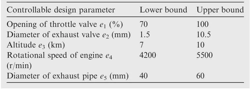
Table 3 Initial simulation conditions for a group of controllable design parameters.

The accuracy of the surrogate model was examined. Note that because the surrogate model is a converted model and it is not appropriate to compare it with experimental results directly, thus the verified simulation models is used to prove the accuracy of the surrogate model indirectly. Fig. 8 shows the relative errors between the surrogate and simulation models. As demonstrated in Fig. 8, the average error between the results generated by the surrogate and original simulation models is 3%for typical parameters(e.g.,the turbine inlet temperature, the rotational speed of the turbocharger rotor, the compressor pressure ratio, and the maximum explosion pressure). The maximum errors for individual parameters are less than 8%.Thus,the errors associated with the use of the surrogate model in the analysis are reasonable and acceptable.Additionally, the errors can be further reduced by increasing the number of sample points.

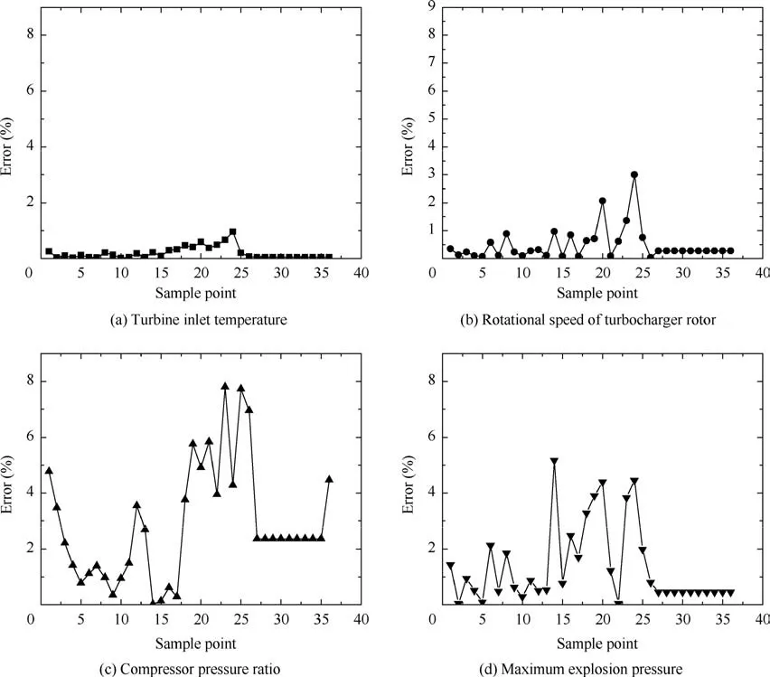
Fig. 8 Relative errors between data generated by surrogate and simulation models for work boundaries of turbocharging system.

5. Results and discussion

To determine the factors affecting abnormal system behaviours, it is necessary to determine the positions of the influencing factors (sample points) under normal conditions (i.e.,the initial sample point cluster). This will serve as the basis for the analysis. Thus, based on the calculation steps of CA described in Section 2.2, a randomly generated N number of sample points (row points) are converted to the form of a type-Q ‘‘factor load matrix” G. Additionally, the cluster consisting of these row points is shown in a 2D scatter plot(Fig. 9). This initial sample point cluster is the precondition for subsequent analysis.

It is worth noting that the failure of a complex system may be attributed to either the independent actions of single influencing factors or the combined action of multiple influencing factors. In this section, abnormal system behaviours caused by the independent actions of single influencing factors are firstly discussed.Then,based on the determined pattern,which is based on single influencing factors, abnormal system behaviours caused by the combined action of two influencing factors are examined. Finally, the analysis is extended to the scenario in which abnormal system behaviours are a result of the combined action of multiple influencing factors.

5.1. Analysis of abnormal system behaviours under independent actions of single influencing factors

To obtain the abnormal data required to analyse abnormal system behaviours under the independent actions of single influencing factors, various factors affecting the sample points are subjected to parametric perturbation within a certain range in order to induce numerical deviations. As a result, the coordinates of the row points deviate along a specific direction.Fig. 10 shows the deviations of the coordinates of the sample points with the change in each influencing factor. Each influencing factor is changed by+20%, +10%, -10%, and-20%, successively.

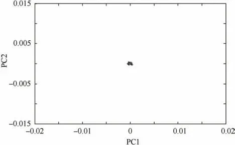
Fig. 9 Positions of sample points during normal system operation in a 2D scatter plot.

As demonstrated in Fig. 10, the relative position of each influencing factor varies to different extents with the extent of the parametric perturbation.In terms of the variation trend,the sample point cluster deviates along the straight line connecting the initial and final positions of its centroid.Additionally, the change in the positive direction (corresponding to an increase) or the negative direction (corresponding to a decrease) of each influencing factor determines the direction of the deviation of the cluster. If the change is increased or decreased at an equal ratio, the sample point cluster will be centrally symmetric to the corresponding initial cluster in the 2D scatter plot. Additionally, the extent of parametric perturbation on each influencing factor also determines the extent of deviation of the sample point cluster from the corresponding initial cluster, i.e., the degree of influence. Specifically, the more significant the parametric perturbation is, the greater the deviation is, and the higher the degree of influence is.The less significant the parametric perturbation is, the smaller the deviation is,and the lower the degree of influence is.Compared to other influencing factors, e2and e4deviate more significantly with parametric perturbation(Fig.10).Based on the identified key factors,corresponding or targeted control strategies can be proposed in future engineering. By comparing the failure rates before and after using the control strategies,it can further verify the influences of the identified key factors.

On the other hand, analysing the independent effects of every single influencing factor will determine its effects on abnormal system behaviours (the extent of deviation of the coordinates).In fact,the deviations of various influencing factors will alter the shape of the row profile.When the changes in each influencing factor with parametric perturbation are reflected in a 2D diagram,the deviation of the cluster will generate various PAs. The 2D scatter plot in Fig. 11 shows the deviations of the sample point cluster as each influencing factor changes by+20%, +10%, -10%, and -20%,successively.

As demonstrated in Fig. 11, as the same influencing factor changes in the same direction but to different extents,the sample point cluster deviates to different extents but at the same PA along the straight line connecting the initial and final positions of its centroid.When different influencing factors change to the same extent in the same direction,the sample point cluster deviates to different extents and at different PAs along the straight line connecting the initial and final positions of its centroid. Positive changes in the influencing factors are further examined. When there are changes to e2and e3, the sample points move towards the first quadrant with a positive change in the deviation.When there are changes to e1and e4,the sample points move towards the fourth quadrant with a positive change in the deviation.When there are changes to e5,the sample points move towards the third quadrant with a positive change in the deviation.Conversely,when the same influencing factor changes to the same extent, the negative and positive changes in the deviation of the sample points are centrally symmetric.

5.2. Analysis of abnormal system behaviours under combined action of two influencing factors

In the previous section,abnormal system behaviours under the independent actions of single influencing factors are analysed.This analysis, in essence, assumes that the influencing factors are independent and do not interact with one another. Under this assumption, the effects of changes in the various influencing factors on the magnitude and direction of the deviation of the sample point cluster are determined. However,in practice,abnormal system behaviours are often the result of the combined action of two influencing factors, i.e., the combined action of two influencing factors when undergoing parametric perturbation (numerical deviation). The magnitude and direction of the deviation of the sample point cluster under the combined action of two influencing factors differ from those under the action of a single influencing factor.

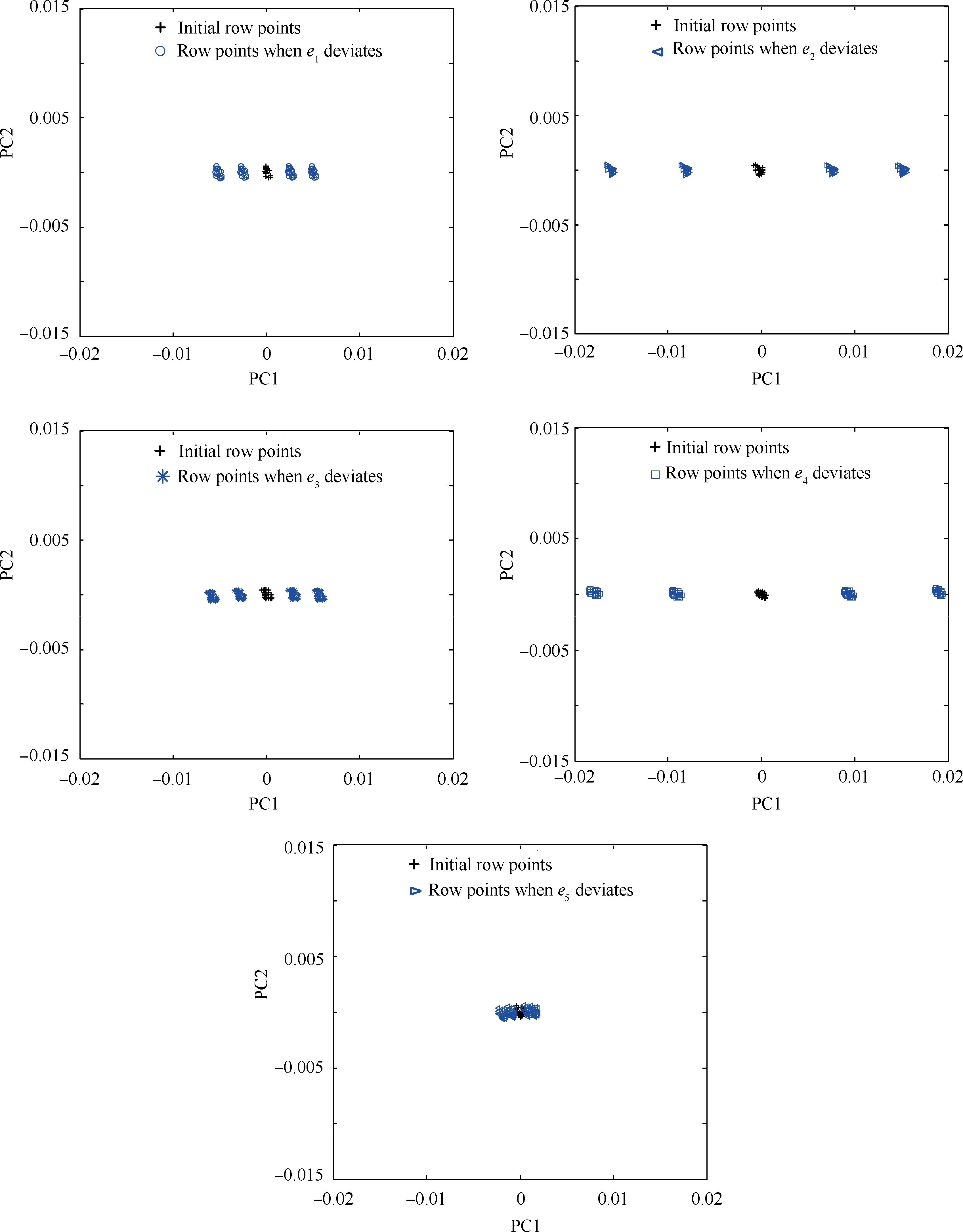
Fig. 10 Extent of change in relative position of each influencing factor with extent of parametric perturbation.

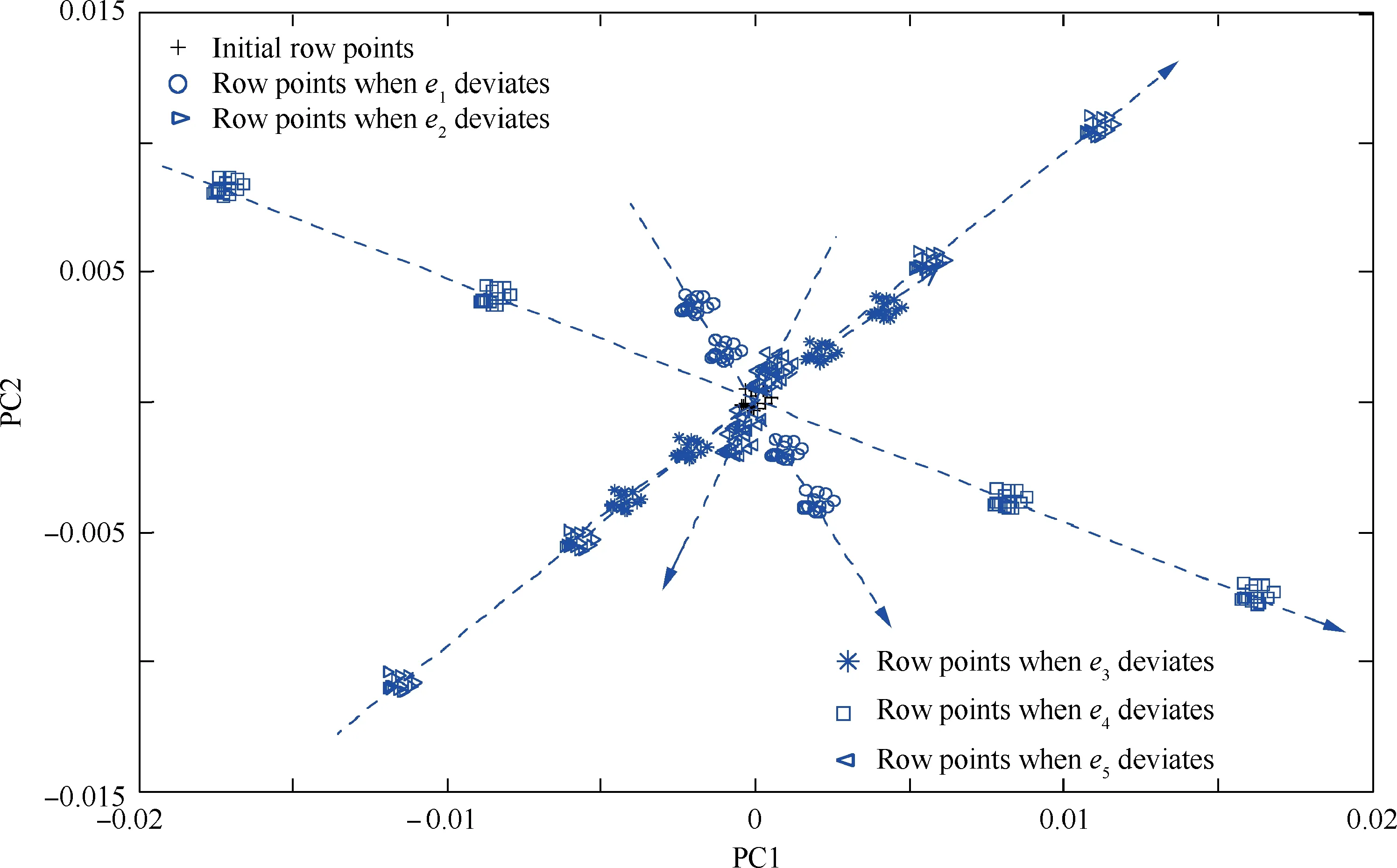
Fig. 11 Deviations of sample point cluster with changes in influencing factors (each influencing factor changes by+20%, +10%,-10%, and -20%).

Additionally, based on the analysis of the independent actions of single influencing factors,e2and e4are the key influencing factors, whereas e1, e3, and e5are the general influencing factors. Therefore, when considering the combined action of two influencing factors, it is necessary to focus on the case where the two influencing factors are both key influencing factors, as well as the case where one of the two influencing factors is a key influencing factor. Additionally, it is also necessary to reflect the changes in the sample point cluster under the actions of single influencing factors as well as the combined action of two influencing factors in one 2D plot for a comparative analysis. This will reveal the difference between the abnormal system behaviours caused by single and multiple influencing factors. These two cases are discussed separately in the following sections.

5.2.1. Combined action of two key influencing factors

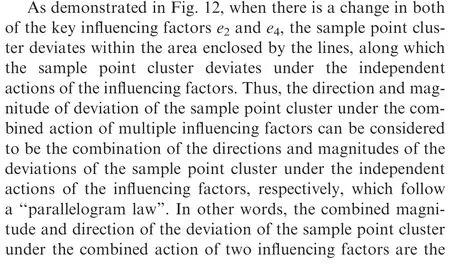
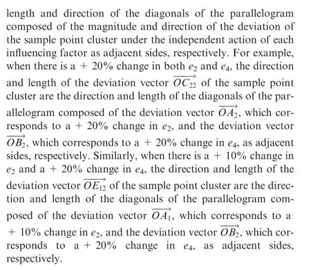
In this section,the first case is analysed using an example of the combined action of two key influencing factors, e2and e4, to study the abnormal system behaviours caused by two influencing factors. Fig. 12 compares the deviations of the sample point cluster under the combined and independent actions of the influencing factors in the following scenarios:(1)when acting together, (A) e2and e4both change by+20%, (B) e2changes by+10% while e4changes by+20%, and (C) e2changes by+20% while e4changes by+10%; (2) when acting individually, e2and e4change by+20%, +10%, -10%,and-20% successively.

5.2.2. Combined action of key and general influencing factors

Similarly, the second case is analysed using an example of the combined action of a key influencing factor e2and a general influencing factor e1to further study abnormal system behaviours caused by two influencing factors. Fig. 13 compares the deviations of the sample point cluster under the combined and independent actions of e2and e1in the following scenarios:(1)when acting together,(A)e2and e1both change by+20%,(B)e2changes by+10%while e1changes by+20%,and(C)e2changes by+20% while e1changes by+10%; (2) when acting individually, e2and e1change by+20%, +10%,-10%, and-20% successively.

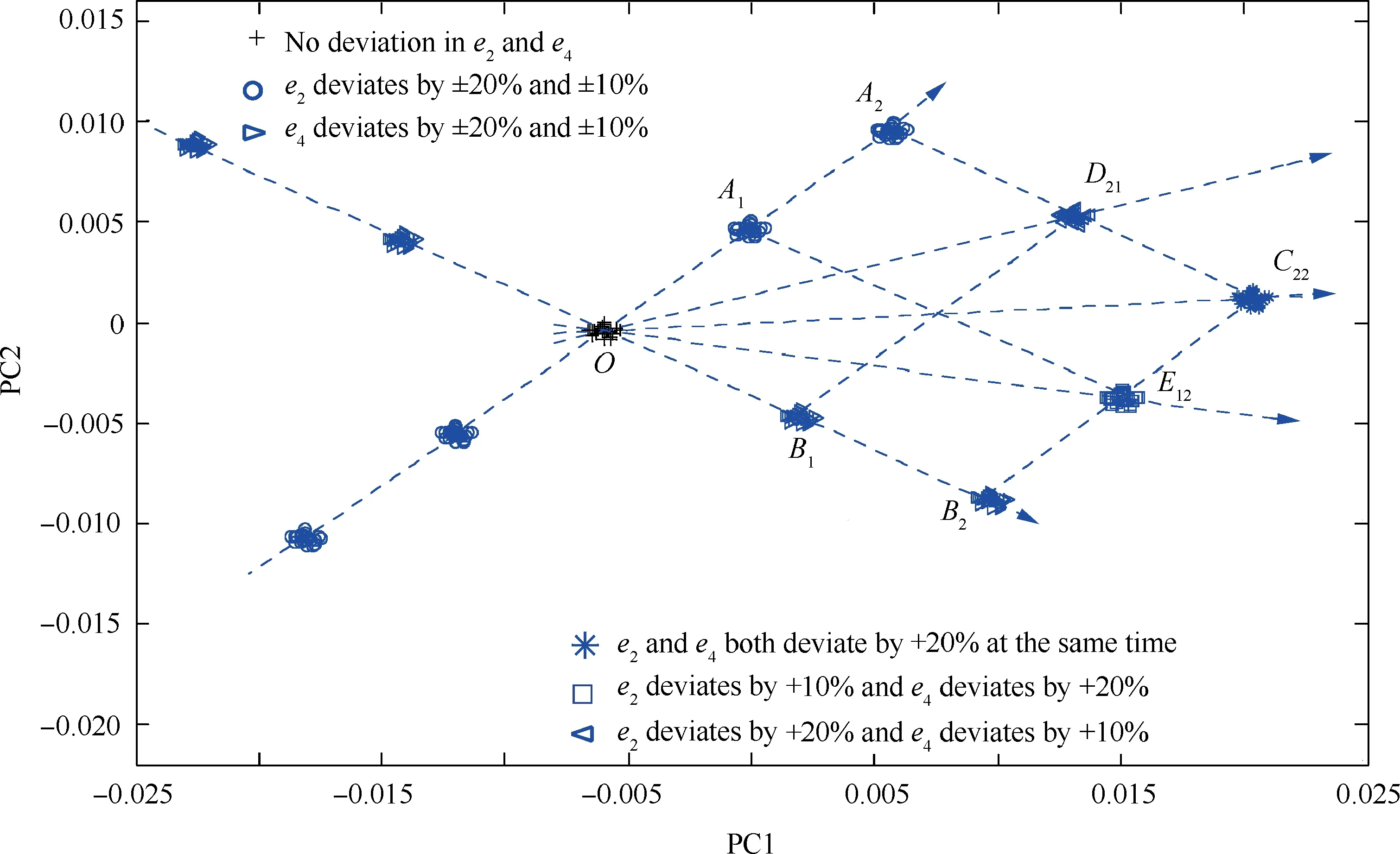
Fig. 12 Comparison between combined and independent effects of key influencing factors e2 and e4.

As demonstrated in Fig. 13, on one hand, when there is a change in both e2and e1, the direction and magnitude of deviation of the sample point cluster also follow the‘‘parallelogram law”.This finding is consistent with that obtained from Fig. 12. On the other hand, when the two influencing factors differ in their degrees of importance but change by the same percentage,the direction of deviation of the sample point cluster is closer to the direction of deviation under the action of the more important influencing factor, i.e., its direction of deviation under the independent action of the key influencing factor.Additionally, the magnitude of deviation of the sample point cluster under the combined action of one key influencing factor and one general factor relies on that under the independent action of the key influencing factor. In other words, the more important a certain influencing factor is, the more significant its impact on the combined direction and magnitude of deviation of the sample point cluster is when acting, together with another influencing factor, on the sample point cluster. Conversely,the less important a certain influencing factor is,the less significant its impact on the combined direction and magnitude of deviation of the sample point cluster is when acting,together with another influencing factor,on the sample point cluster.On this basis,it can be further inferred that when the two influencing factors each have a relatively low degree of importance(i.e., when two general influencing factors act together), the combined magnitude of deviation of the sample point cluster is also relatively small. Therefore, it is necessary to control the key influencing factor when two influencing factors act together.

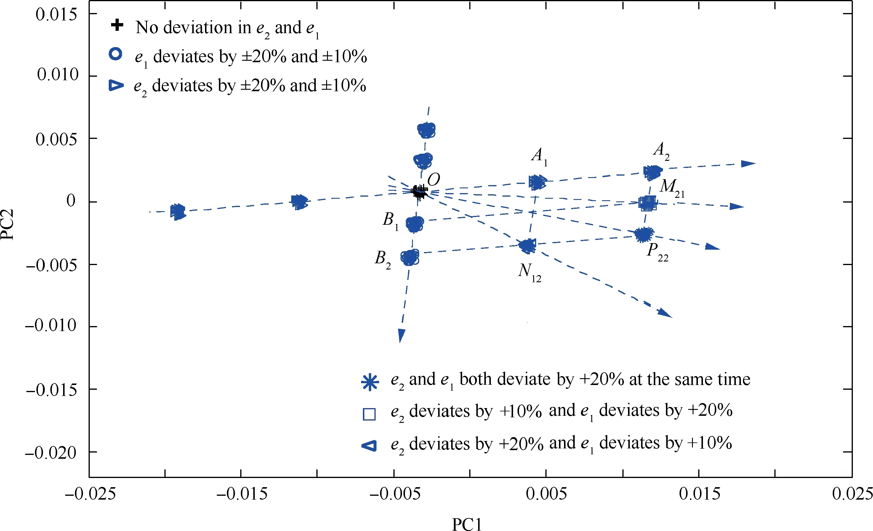
Fig. 13 Comparison between combined and independent effects of a key influencing factor e2 and a general influencing factor e1.

5.3. Analysis of abnormal system behaviours under combined action of multiple influencing factors

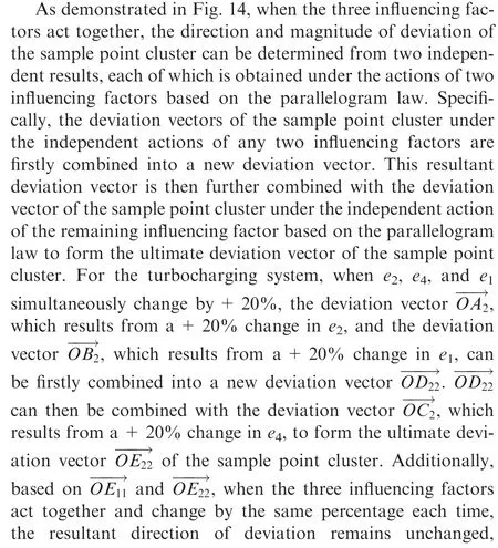
Based on the analysis in Sections 5.1 and 5.2, under the independent action of each influencing factor, the sample point cluster deviates along the straight line connecting the final and initial positions of its centroid.Under the combined action of two influencing factors, the direction and magnitude of deviation of the sample point cluster follow the‘‘parallelogram law”and are more significantly affected by the key influencing factor. While it is very common that two influencing factors act together in practice, there are still cases where three, four,or even five influencing factors act together. Therefore, to study the pattern associated with the direction and magnitude of deviation of the sample point cluster under the combined action of multiple influencing factors,three influencing factors for the turbocharging system are selected, and the results under their combined action are analysed. It is worth noting that the analysis of the combined action of two influencing factors shows that the deviation of a sample point cluster is relatively more significantly affected by the key influencing factor.Thus,when studying the combined action of multiple influencing factors,two key influencing factors,e2and e4,and one general influencing factor, e1, are selected for analysis. Fig. 14 shows the deviations of the sample point cluster with changes in the three influencing factors when they act together or individually in the following scenarios: (A) when acting together,e2, e4, and e1change by+20% or+10%; (B) when acting individually, e2, e4, and e1successively change by+20%,+10%, -10%, and-20%.

Moreover, based on the above results, the difference between the deviations of the sample point cluster caused by changes in the general and key influencing factors can be further analysed.

5.3.1. Effects of changes in general influencing factors on

deviation of sample point cluster

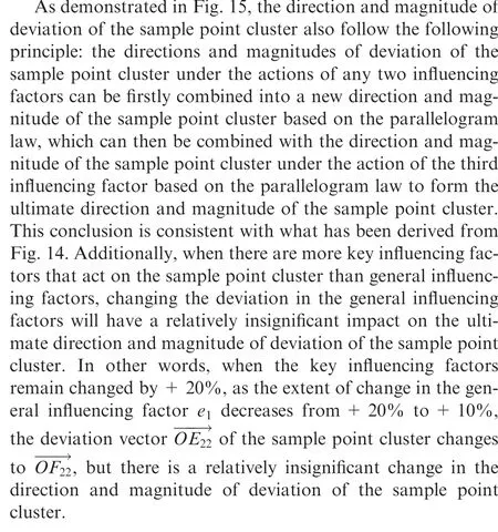
In the above analysis,if the extent of change in each of the key influencing factors e2and e4remains unchanged at+20%,reducing the extent of change in the general influencing factor e1from+20%to+10%will further reflect the effects of the general influencing factors on the deviation of the sample point cluster. Fig. 15 compares the deviations of the sample point cluster caused by changes in e1in these two cases.

5.3.2. Effects of changes in key influencing factors on deviation of sample point cluster

However,if the extents of change in the key influencing factor e4and the general influencing factor e1remain unchanged at 20% and+10%, respectively, reducing the extent of change in the key influencing factor e2from+20% to+10% can further reflect the effect of the key influencing factor on the deviation of the sample point cluster. Fig. 16 compares the deviations of the sample point cluster with a numerical change in the key influencing factor e2in these two cases.

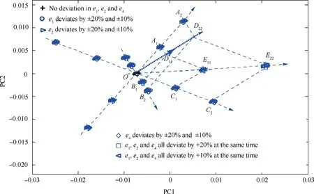
Fig.14 Comparison of deviations of sample point cluster under combined(e2,e4,and e1 all simultaneously change+20%or+10%)and independent (e2, e4, and e1 individually change by+20%, +10%, -10%, and-20%, successively) actions of influencing factors.

Fig. 15 Comparison of deviations of sample point cluster under combined and independent actions of influencing factors (extent of change in each of key influencing factors e2 and e4 remains unchanged at+20%, while extent of change in general influencing factor e1 decreases from+20% to+10%).

A comparison between the results derived from Figs.14-16 shows that when multiple influencing factors act together, the direction and magnitude of deviation of the sample point cluster can still be determined based on the parallelogram law.Additionally, changes in the key influencing factors play a main role in the direction and magnitude of deviation of the sample point cluster, whereas changes in the general influencing factors affect the sample point cluster relatively insignificantly.

in key influencing factor e4and general influencing factor e1remain unchanged at+20% and+10%, respectively)

6. Conclusions

In view of the general aircraft safety issues caused by aviation piston engine turbocharger failure, this study focuses on a method for determining turbocharge failure-inducing factors.A whole-machine (engine and turbocharger) system model is established. On this basis, an improved CA-PAC method is proposed to determine the key factors affecting the failure mode of aviation piston engine turbochargers. This method provides a new means for accurately formulating failure risk control strategies for practical operation and maintenance.The results of this study are summarized as follows:

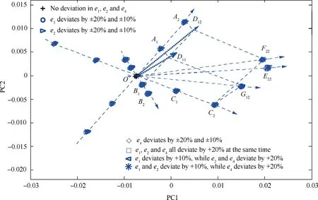
Fig. 16 Comparison of deviations of sample point cluster under combined and independent actions of influencing factors (extent of change in key influencing factors e2 decreases from+20% to+10%, while extents of change in key influencing factor e4 and general influencing factor e1 remain unchanged at +20% and +10%, respectively).

(1) In the proposed improved CA-PAC method, the factor identification method based on the variation of the row profile coordinates G with the numerical deviations of the key influencing factors is capable of effectively identifying the key failure-affecting factors. Specifically,by examining the magnitude and direction of the deviation of the sample point cluster that represents the safety margin for each work boundary from its position under normal conditions, potential single or multiple factors causing the deviation of the sample point cluster can be determined. Thus, key influencing factors are determined. In this basis, targeted failure risk control strategies can be accurately formulated in practical operation and maintenance.

(2) The accuracy of the proposed method depends on the accuracy of the system model,and thus the model is validated through an experimental comparison. However,to reduce the computational cost of CA, the response surface method is further employed to abstract the system simulation model into a surrogate model. The final average error of the surrogate model is approximately 3%. This ensures accuracy while reducing the computational cost.

(3) For the turbocharging system example examined in this study, the diameter of the exhaust valve (e2) is the primary factor affecting the safety margin for each work boundary. Thus, e2is the key influencing factor and needs to be controlled firstly in application and maintenance.

Declaration of Competing Interest

The authors declare that they have no known competing financial interests or personal relationships that could have appeared to influence the work reported in this paper.

Acknowledgements

The work was supported by the Innovation Team of Complex System Safety and Airworthiness of Aeroengine from the Co-Innovation Center for Advanced Aeroengine of China. The work was funded by the National Natural Science Foundation of China and the Civil Aviation Administration of China(No.U1833109).

Appendix A. The basic principle and calculation steps of CA are described as follows:

A.1. Original matrix establishment

Let there be n samples in the contingency table. Each sample observes p indices. Thus, the corresponding original matrix X is as follows:

where xijis the value of the jth index in the ith sample.

A.2. Elimination of error caused by difference in dimension between variables

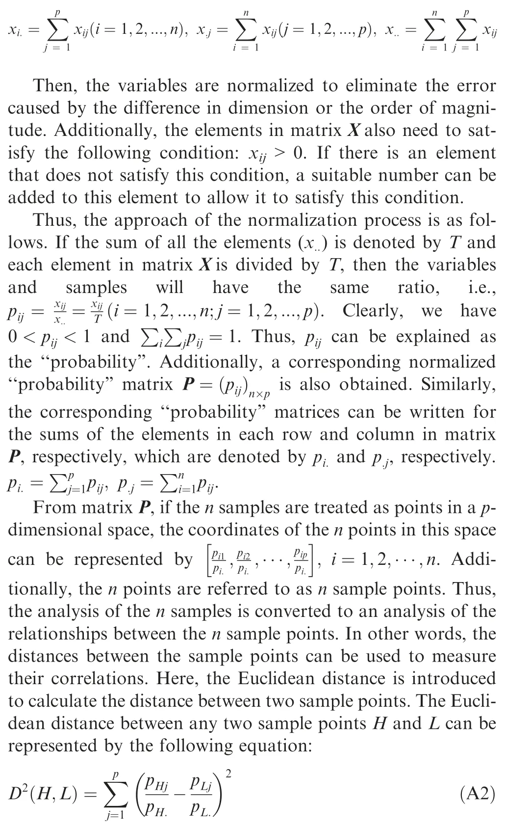
Firstly, the sum of the elements in each row in matrix X,the sum of the elements in each column of matrix X, and the sum of all the elements in matrix X are further given,which are denoted by xi., x.j, and x.., respectively. That is

A.3. Elimination of error caused by difference in order of magnitude between variables

To eliminate the error caused by the difference in the order of magnitude between variables(e.g.,if the Hth variable has a relatively large order of magnitude, this variable will increase the error when calculating the distances between the sample points due to its larger scale of effect),the concept of weighted distance (or chi-square distance) is introduced to the analysis.The weighted distance between any two sample points H and L can be represented by the following equation:

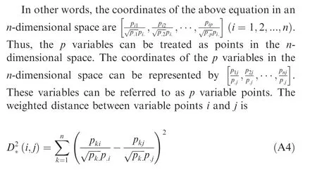
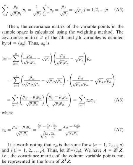
The sample or variable points can be classified by calculating the distance between every two sample or variable points.However, because these sample or variable points have ndimensional coordinates, they cannot be simply and visually represented by a two-dimensional (2D) plot. Thus, to use a 2D plot to visually show the relations between the variable and sample points,it is necessary to further introduce the concepts of variable point covariation matrix and sample point covariation matrix.

Firstly,the ith variable point is weighted based on the probability pi.as

Similarly,the covariance matrix of the row sample points is denoted by B=(bHL). bHLis

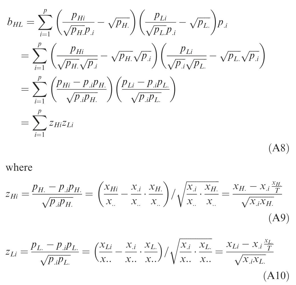
We have B=ZZT, i.e., the covariance matrix of the row variable points can be represented in the form of ZZT.

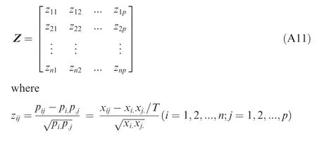
In summary,after the original matrix X is transformed,the covariance matrices of the column and row variable points can be represented by A=ZTZ and B=ZZT,respectively.There is a clear corresponding relation between matrices A and B.Thus, on one hand, the variable and sample points can be reflected on a plane determined by the same factor axis (i.e.,in the same coordinate system). On the other hand, after the original data point xijis transformed to zij, because zijis the same for i and j, zijis the same for the variable and sample,i.e.,Z is the same for the variables and samples.Thus,the original matrix X can be transformed into a new matrix Z as

A.4. R and Q factor analysis

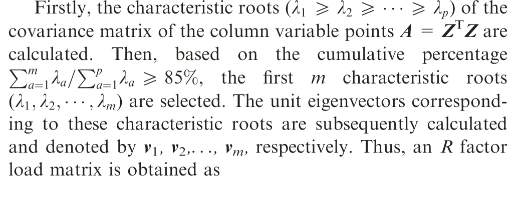
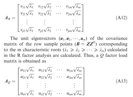
The original matrix X is transformed into matrix Z in the above analysis.On this basis,the required R and Q factor analysis is established.

A.5. Determination of a 2D plot for Correspondence Analysis(CA)

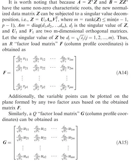
Additionally,the sample points can be plotted on the plane formed by any two factor axes based on the obtained matrix G.

In summary,when m=2,the first two columns of the‘‘factor load matrix” G contain the coordinates of each row point(sample point) in the 2D representation (optimum data). The first two columns of the ‘‘factor load matrix” F contain the coordinates of each column point (variable point) in the 2D representation (optimum data). Therefore, a point plot is produced on the same 2D plane using the row profile coordinates G and the column profile coordinates F,as shown in Fig.A1.It is worth noting that the Euclidean distances between the points in Fig. A1 correspond to the weighted distances between the original data row (or column) profiles. Thus, based on the proximity between points, the variable and sample points can be considered at the same time during the analysis and also be further subjected to a classification analysis.

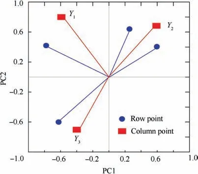
Fig. A1 2D scatter plot for CA.