Two new multi-phase reliability growth models from the perspective of time between failures and their applications

Kunsong LIN, Yunxia CHEN,*

a School of Reliability and Systems Engineering, Beihang University, Beijing 100191, China

b Science and Technology on Reliability and Environmental Engineering Laboratory, Beihang University, Beijing 100191, China

KEYWORDS Reliability growth;Test-find-test strategy;Test-fix-test strategy;Time-varying failure intensity;Time between failures

Abstract Aviation products would go through a multi-phase improvement in reliability performance during the research and development process.In the literature,most of the existing reliability growth models assume a constant failure intensity in each test phase, which inevitably limits the scope of the application. To address this problem, we propose two new models considering timevarying failure intensity in each stage. The proposed models borrow the idea from the accelerated failure-time models. It is assumed that time between failures follow the log-location-scale distribution and the scale parameters in each phase do not change,which forms the basis for integrating the data from all test stages.For the test-find-test scenario,an improvement factor is introduced to construct the relationship between two successive location parameters.Whereas for the test-fix-test scenario, the instantaneous cumulative time between failures is assumed to be consistent with Duane model and derive the formulation of location parameter. Likelihood ratio test is further utilized to test whether the assumption of constant failure intensity in each phase is suitable. Several applications with real reliability growth data show that the assumptions are reasonable and the proposed models outperform the existing models.

1. Introduction

Reliability assessment of products before their launch onto the market has always been an interest of manufacturers as it is one of the critical factors for decision-making.1,2During the Research and Development (R&D) process, most aviation products would go through an improvement in reliability performance over time due to the implementation of corrective actions or fixes to design, operation, maintenance procedures,or the associated manufacturing process.3-5With the development of products, failure data tend to be fewer and fewer and even none,as the reliability of the final configuration is extremely high.6,7Using such small samples to predict reliability would lead to an assessment with tremendous uncertainty. Hence, it is natural for scientists and engineers to find a way to use all the data generated in R&D process to obtain a more accurate prediction.8

Reliability Growth (RG) modelling is a valuable tool to describe such a process and has been an area of great interest.Duane introduced one of the most famous empirical models in 1964.9He found that the cumulative failure rate is linear to the cumulative test time on the log-log plot. Crow interpreted the Duane model with a stochastic process and then developed the AMSAA model, which is also known as the power-law model or Weibull process model.10He also used the historical data to obtain some information to plan a better reliability growth program11and further extended the model to a discrete system.12Hall and Mosleh developed a framework for the reliability growth of a one-shot system.13Hall et al. further extended it for discrete use systems.14

Recently, Li et al. utilized a Bayesian method to assess the product reliability and argued that the prior distribution from the rough experience of product designers or experts cannot guarantee the forecast accuracy.15Therefore,a four-step modelling method was proposed to build a reliability growth model for new products without assuming prior distribution.Jin et al.studied the effects caused by latent failures due to design immaturity and uncertain operating conditions.16Wayne and Modarres built a Bayesian model for complex system reliability growth under arbitrary corrective actions.17It was assumed that the system has several independent failure modes and the failure intensity for each model is constant both before and after the implementation of corrective actions. Li et al. optimized the multi-stage reliability growth with multiple objectives in the early product-development stage18and Mobin et al.further considered the effect of introducing new technologies.19Byun et al. used a matrix-based method to model the reliability growth of a k-out-of-N system.20Tafaluse and Pohl utilized a grey system model to deal with the case of tiny sample size.21,22Ruiz et al. developed a Bayesian framework to assess accelerated reliability growth with multiple sources of uncertainty.23Saraf and Iqbal proposed a new software reliability growth model with the consideration of imperfect debugging and change points.24Pandian et al. utilized the AMSAA model to conduct a reliability growth analysis on Boeing 787 Dreamliner.25For a detailed review of the RG models, please refer to the work of Wayne26and Jiang.27

With their development, the RG models tend to be more complicated to adapt for various conditions in reality. However, most RG models are formulated in terms of the failure rate(or intensity)reduction,typically based on the assumption that failure intensity of the products with the same configuration is constant.5,28Such an assumption is often violated in reality. It is well known that the lifetime distribution of nonrepairable products is more likely to be non-exponential.

To overcome the above limitations,we model the reliability growth process from the perspective of the Time Between Failures (TBF) instead of the failure intensity and propose two new reliability growth models regarding the test-find-test strategy and test-fix-test strategy, respectively. We assume that the TBF in each test phase follows a log-location-scale distribution. With this assumption, the failure intensity is timevarying even in the same test phase, which is more consistent with real situations. Moreover, we borrow the idea of the Accelerated Failure-Time Model (AFTM) and further assume that the corrective actions would only change the location parameter but not affect the scale parameter.This assumption constructs the relations between failure data among different test phases. Hence, we can use all the test data to predict the reliability of products in the final configuration. It is also proved reasonable in our case study, where the comparison clearly shows that the proposed model outperforms the existing models.

The remainder of this paper is structured as follows.Section 2 introduces the ideas of the models and then develops two models. Parameter estimation methods are given in Section 3. Section 4 demonstrates the validity of the proposed models based on three sets of real data. Some concluding remarks are given in Section 5.

2. Model development

2.1. A different insight into reliability growth

Most existing RG models tend to describe reliability improvement from the perspective of failure intensity.Specifically,it is usually assumed that the failure intensity is constant both before and after the implementation of corrective actions,and the failure intensity after corrective action is reduced to a lower level, e.g., see the work of Wayne26. Then the whole reliability improvement process could be regarded as an idealized continuous growth curve.The basic idea of these models is presented in Fig. 1.

This paper, instead, models the reliability improvement from the perspective of TBF.We assume that the TBF follows a log-location-scale distribution, and the corrective actions would only change the location parameter but not affect the scale parameter, as presented in Fig. 2. The corrective actions at the end of each phase cause the TBF distribution to have a left shift but with the shape unchanged.

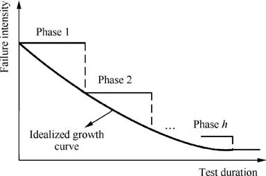
Fig. 1 Basic ideas of existing RG models.

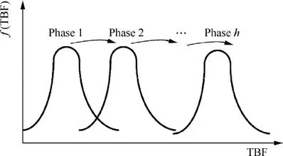
Fig. 2 Basic ideas of proposed models.

This idea comes from AFTM. In an Accelerated Life Test(ALT), the applied stresses are raised to the higher levels,but still under the stress limits. The product failure time becomes shorter under high stress level, whereas the failure mechanisms remain unchanged. We use the Stress-Strength Inference (SSI) model to describe this phenomenon. Fig. 3(a)shows that the strength of several samples belonging to the same population s0decreases with time gradually.The samples would fail when the strength is equal to the stress σs0. For example, the sample with medium strength would fail at the time t0.We record every lifetime and obtain the lifetime distribution afterward. In the ALT, if the stress is raised to σs1and σs2, the sample failure time is shortened to t1and t2, respectively. Hence, the lifetime distribution is shifted left. In this case, it is usually assumed that stress would only affect the location parameter and the scale parameters under different stress levels are the same,the latter of which implies the invariant failure mechanism.

During the RG progress, the reliability performance is improved by mitigating some failure modes. One typical way is to enhance the strength of the products.Fig.3(b)shows that the product with strength s0would fail at the time t0under stress σs0. The lifetime distribution can be obtained for a population.In the RG process,the corrective actions at the end of phase zero and phase one would increase the strength from the initial s0to s1and then to s2,respectively,with the corresponding failure time from t0to t1and t2,respectively.Hence the distribution would have a right shift.For this reason,the process can be regarded as an inverse process of ALT, which leads to the idea that the fixing actions would only affect the location parameter without changing the shape parameter.

2.2. Assumptions

Suppose that the products undergo h test phases, and corrective actions are implemented at the end of the previous h-1 phases.That is,the states of the products in a particular phase stay exactly the same. Once corrective action is implemented,the (i-1)th test phase would turn into the ith one and the state changes.

Based on the idea above,the assumptions for the model are given as follows:

(1) All failures occur independently,and TBFs in the ith test phase follow the same log-location-scale distribution with the location parameter μiand the scale parameter σi.

(2) Corrective actions at the end of the ith test phase would affect the location parameter μiby a function of g (μi).

(3) σiis constant (=σ) and independent of test phase.

2.3. Model formulation

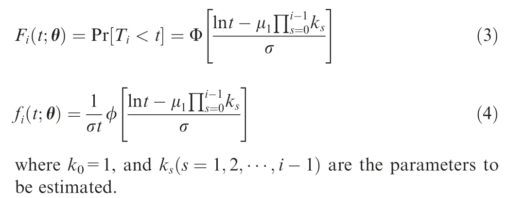
According to the assumptions above,the Cumulative Distribution Function(CDF)and Probability Density Function(PDF)of TBF are, respectively, given by

where Φ denotes a standard CDF(e.g.,standard normal distribution), and φ is the corresponding PDF.

Scenario 1. Test-find-test strategy

During the RG test, the strategy that all correction actions are delayed until the end of the test is called the test-find-test strategy.That is,the failed products are repaired and put back to the chamber until the end.At the end of the test,the corrective actions are implemented to mitigate the failure modes. It should be noted that repairs do not change the design of the products,whereas the corrective actions do.Hence the reliability of the products improves only by corrective actions.In that case, we assume that corrective actions at the end of each test phase make the reliability performance jump to a higher level with an improvement factor ki, i.e. μi+1= kiμi. Then the CDF and PDF of TBF in the ith test phase are respectively expressed as

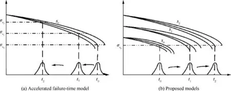
Fig. 3 Relationship between accelerated failure-time model and proposed models.

Note that the log-location-scale distribution family contains some well-known distributions,including the Weibull distribution, exponential distribution, and lognormal distribution. In what follows, we give specific expressions for different distributions.

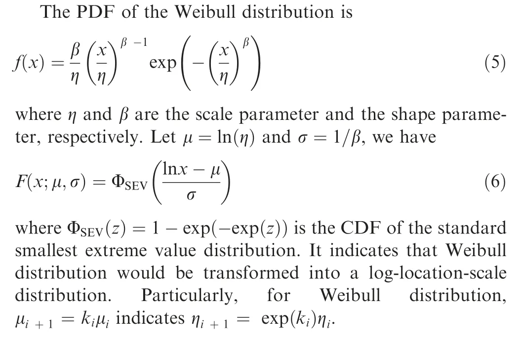
Case 1. Weibull distribution Case 2. Exponential distribution

The exponential distribution is a special case of Weibull distribution. Hence, it also belongs to the log-location-scale distribution family. The PDF of the exponential distribution is given by

Case 3. Lognormal distribution

The PDF of the lognormal distribution is given by

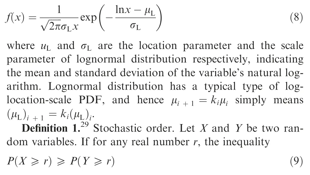
holds, then X is stochastically greater than or equal to Y, or X≥stY.Equivalently, Y is stochastically smaller than or equal to X, or Y≤stX.

Scenario 2. Test-fix-test strategy

In the test-fix-test strategy, failure modes are revealed during testing, and corrective actions for these problems are implemented immediately. Then the reliability growth can be approximated as a continual improvement process characterized by a smooth curve,which is also considered in most existing RG model, e.g. the Duane model and AMASS model.Hence,the location parameter μ is a continual function of time t. Theoretically, μ(t ) can be of arbitrary form, incurring a problem of function selection. Considering that the Duane model, as the most well-known empirical RG model, has become the basis for a number of other RG models, e.g.,AMASS. Hence, we also would like to make the results of our model consistent with the Duane model. That is, the instantaneous cumulative time between failures is linear to the cumulative test time on a log-log scale plot. Specifically,

where a is a constant, and the m is the slope on a log-log plot representing the reliability growth rate.

Since Mean Time Between Failures (MTBF) in our model depends on the specific type of the distribution, we further specify the forms of the μ(t ) for three most widely used loglocation-scale distributions in reliability engineering, i.e., Weibull distribution, exponential distribution, and lognormal distribution in the following contents.

Case 1. Weibull distribution

The expectation of the Weibull distribution is given by

where Γ(·) is a gamma function

Therefore, we let

That is

Case 2. Exponential distribution

The expectation of the exponential distribution is given by

Therefore, we let

Comparing Eq. (18) with Eq. (12), it can be found that the model in this case is consistent with the Duane model.

Case 3. Lognormal distribution

The expectation of the lognormal distribution is given by

Therefore, we let

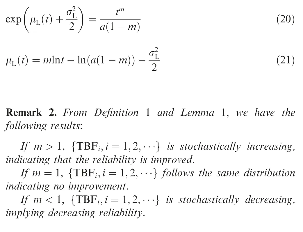
Remark 3. It should be noted that there are several assumptions in the proposed models.The first assumption is the log-locationscale distribution family.Therefore,if the family cannot provide a satisfying fit,the proposed models should not be used.The third assumption is even stricter. Therefore, for scenario 1, we would further provide a test method to verify whether the hypothesis is acceptable.As for scenario 2,we can only verify it by comparing it with the existing models, e.g., AMSAA model. Some recent studies have considered non-constant shape parameters in AFTMs. Therefore, if the data do not satisfy the third assumption, then an RG model with non-constant scale parameter should be further considered.

3. Parameter estimation and reliability evaluation

In this section, we employ the Maximum Likelihood Estimation (MLE) method to estimate the parameters of the two models.

3.1. MLE for parameters of the model in scenario 1

Consider that the RG test contains h test phase, and there are nisamples in the ith test phase.Suppose that the pth system in the ith test phase (denoted as ip) works from time 0 until Tipand has failed for niptimes at time points sip，j, with j=0， 1， 2， ···， nip. Let sij，0= 0. Then TBFs of system ip are sip，1-sip，0,...,sip，nip-sip，nip-1,and Tip-sip，nip,respectively. Denote tipj=sip，j-sip，j-1. Then the log-likelihood function is

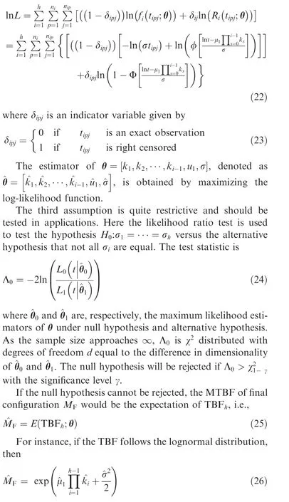
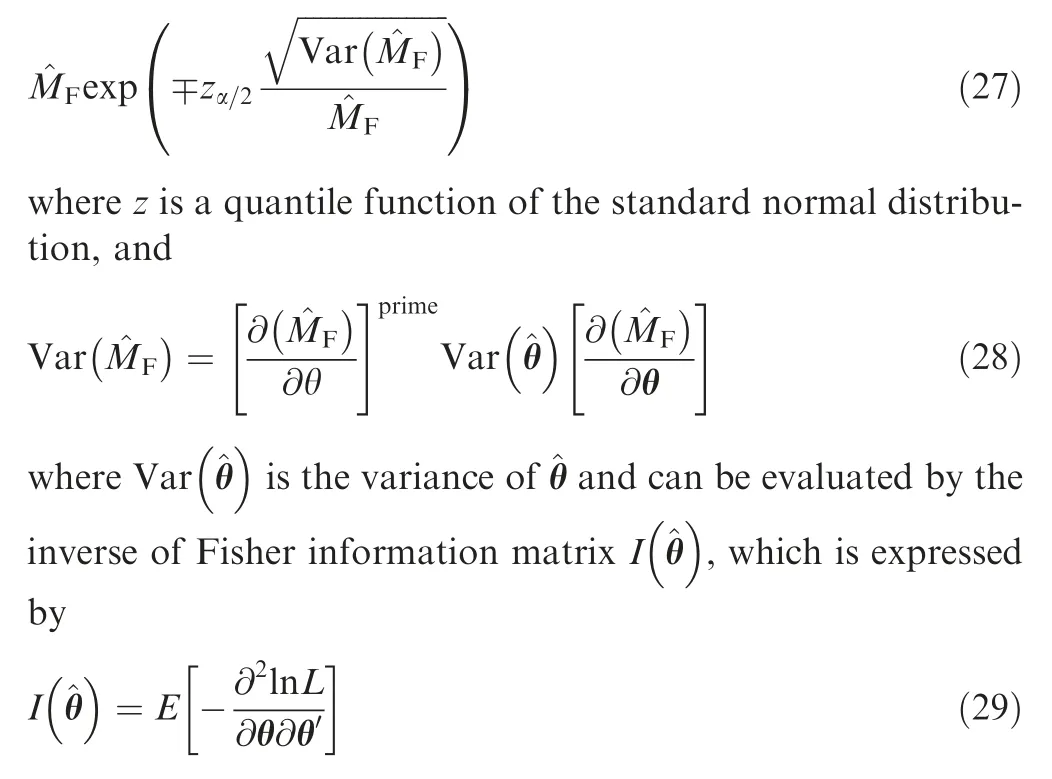
The 1-α confidence interval of MFis

3.2. MLE for parameters of the model in scenario 2

Consider that n systems are in test. Suppose that system p works from time 0 until Tpand has failed for nptimes at time points Sp,j, with j=0，1，2，···，np. Let sj，0=0. Then TBFs of system p are sp，1-sp，0,...,sp，np-sp，np-1, and Tp-sp，np, respectively. Denote tpj=sp，j-sp，j-1. Then the log-likelihood function is

Specifically, for Weibull distribution, it can be written as

Using Eqs. (27) and (29), we can obtain the lower confidence bound of the MTBF.

4. Applications

In this section,two examples with real-world datasets are illustrated to compare the performance of the proposed models with that of the existing models in terms of Akaike Information Criterion(AIC).In the following contents,we will denote the proposed models for the test-find-test strategy as model I and the test-find-test strategy model II. Section 4.1 gives a set of real data to verify the validity of model I, and the likelihood ratio test is conducted to test the validity of the third assumption, whereas Section 4.2 utilizes two sets of data in the existing literature to verify the validity of model II.

4.1. Case 1

An engine was subject to a three-phase reliability growth test with two groups of critical corrective actions at the end of the first and second test phases. The observed (censored) time between failures is presented in Table 1.

We use three commonly used log-location-scale distributions (the exponential, lognormal and Weibull distribution)to fit the data and select a best-fitted one based on AIC,which is

where l is the number of the independent parameters. The smallest AIC value indicates the best fitted model. MLEs of parameters and the AIC values are given in Table 2. It can be observed that the exponential distribution has the largest AIC value. Meanwhile, there is a serious deviation between the fitted curve and the data in the right tail(see Fig.4),which implies that the assumption of a constant failure rate is not reasonable. It should be noted that such an assumption is widely used in the existing models,e.g.,AMSAA maturity projection model30and the one in a recent work.17The lognormal distribution outperforms the exponential and Weibull distributions as the AIC value of the lognormal distribution (i.e.,1527.6) is the smallest. Fig. 5 shows that the lognormal distribution can provide a satisfying fit.It also presents that the fixing actions at the end of phase 2 have better improvement than the ones in phase 1 as the distance between the blue line and green line is much larger than the one between the green lineNote: σ≡1 in exponential distribution.and the red line. Table 2 also shows that k2is larger than k1.Therefore, the graphic can provide an intuitive reliability growth result. In the following analysis, the lognormal distribution is adopted as the TBF distribution.

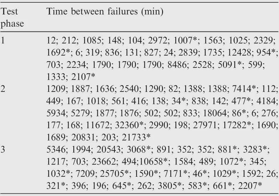
Table 1 Time between failures from RGT.

Table 2 Parameter estimates and performance of three models.

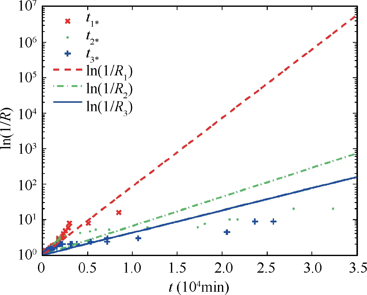
Fig. 4 MLE and non-parametric estimates of system reliability for exponential distribution.

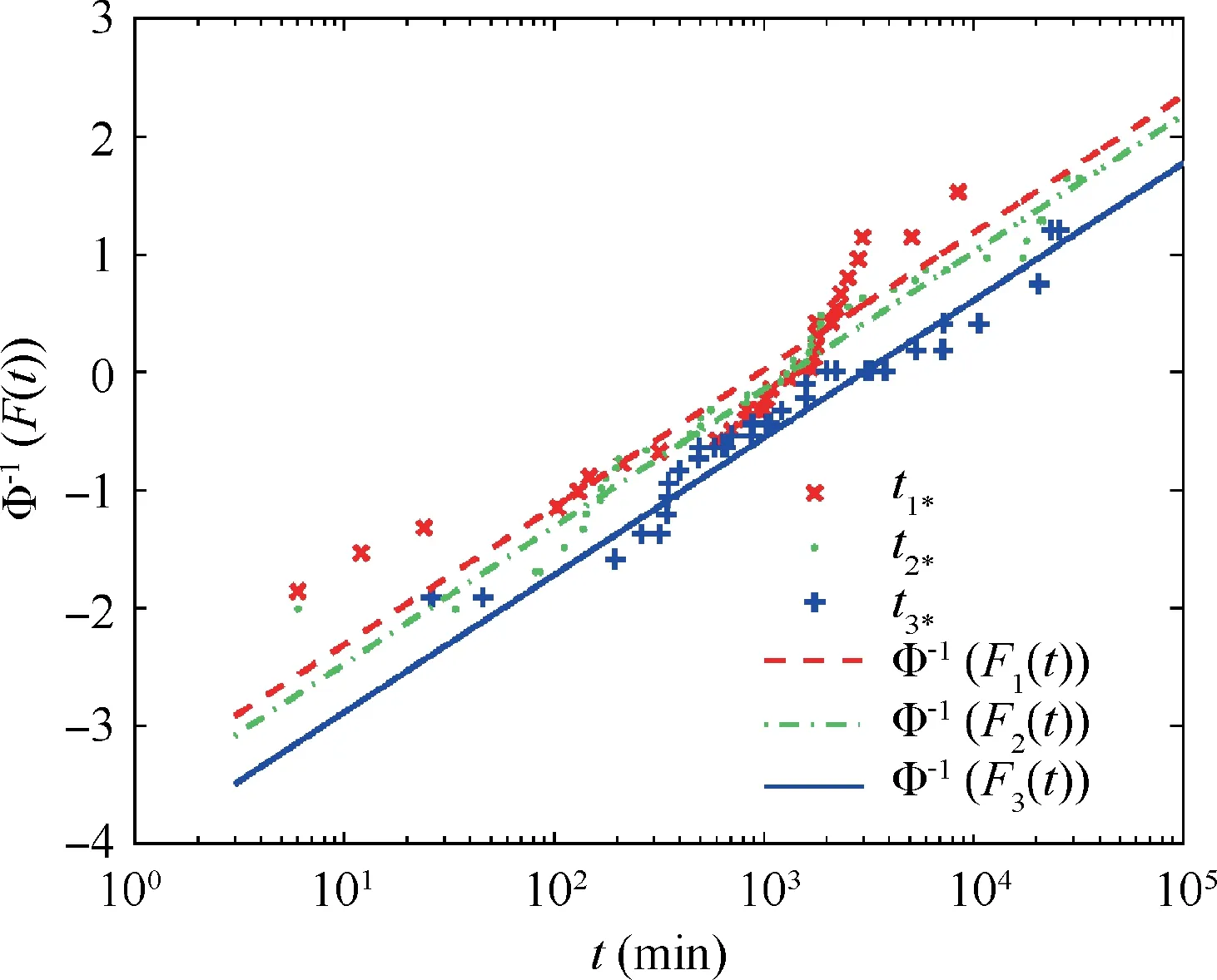
Fig. 5 MLE and non-parametric estimates of system reliability for lognormal distribution.

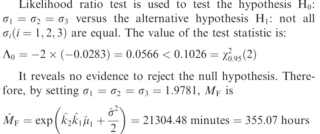
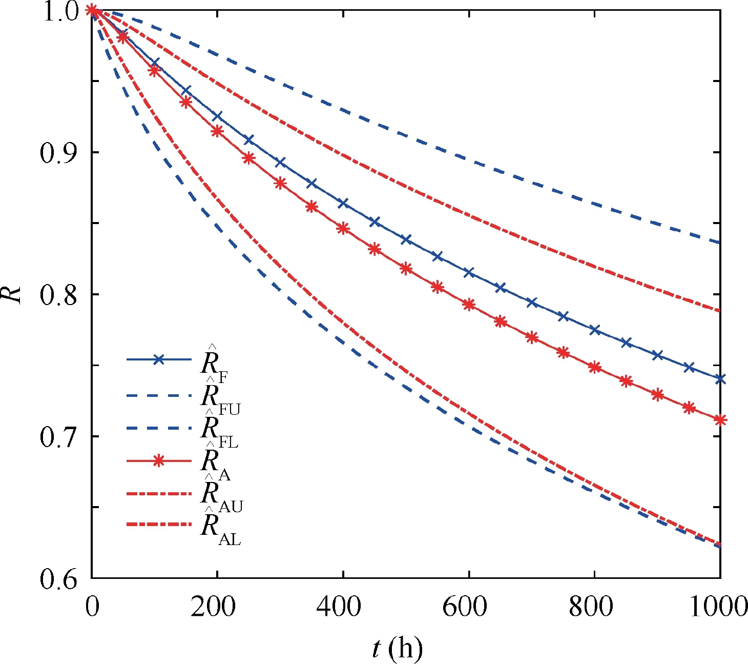
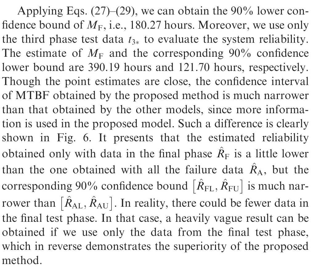
Fig. 6 Point estimates and confidence bound of the reliability obtained by proposed method and the one using only the data in final phase.

4.2. Case 2

Hossain and Dahiya presented 34 software failure data,including the TBFs and cumulative failure time.31Crow gave 40 failure times of a system tested for 3256.3 hours.32The transformed TBFs are given in Table 3.

On these two TBF datasets,we use the MLE to estimate the parameters and then compare the performance of the proposed model with AMSAA model,which is the most widely used reliability growth model in the exiting literature. The likelihoodfunction of AMSAA model can be referred to in the work of Crow.33The parameter estimates and the corresponding AIC values are given in Tables 4 and 5.It is noted that the numbers of the parameters in the proposed model II are 2,3,3 for exponential, Weibull, and lognormal distributions, respectively.For AMSAA model,l=2.Both tables show that the proposed models outperform the Duane model and AMSAA model.Specifically,for software failure data,the proposed model with lognormal distribution has the best performance, whereas the proposed model with Weibull distribution performs better than the other three models for the second dataset. According to this result,the mean time to failure of final configuration for two systems are

Table 3 Transformed TBFs from failure time data in Ref.32

Table 4 Parameter estimation and AIC values of four models for the first dataset

Table 5 Parameter estimation and AIC values of four models for the second dataset.

with the corresponding 90% lower confidence bound as 17.09 hours and 117.39 hours respectively.

5. Conclusions

This paper proposes two reliability growth models. Instead of modeling the reliability improvement progress based on the constant failure intensity, the proposed models capture the trend of reliability growth from the perspective of time between failures. Specifically, this paper borrows the idea of the accelerated failure-time model and assumes that TBF follows a general log-location-scale distribution indicating a time-varying failure intensity. We also assume that corrective actions would only affect the location parameter but not change the scale parameter.Furthermore,we specify the models in two scenarios, i.e., the system is improved with a testfind-test strategy and test-fix-test strategy. Our case study shows that the proposed models outperform the existing ones,and a likelihood ratio test is utilized to verify that the assumption of constant scale parameter is appropriate.

Our future work aims to construct a reliability growth model under arbitrary corrective actions. Another possible research focus is to develop an RG model with the nonconstant scale parameters.The last but not least point is to utilize both the lab test data and field test data during the R&D progress to develop a more general model.

Declaration of Competing Interest

The authors declare that they have no known competing financial interests or personal relationships that could have appeared to influence the work reported in this paper.

Acknowledgements

The authors thank the anonymous reviewers for their critical and constructive review of the manuscript. This study was co-supported by the National Natural Science Foundation of China (No. 52075019) and the Academic Excellence Foundation of BUAA for PhD Students, China.