An experimental method to obtain the hard alpha anomaly distribution for titanium alloy aeroengine disks

Shuiting DING, Huimin ZHOU, Boho PAN, Hiin JI, Xiojun GUO,Guo LI,*

a Aircraft/Engine Integrated System Safety Beijing Key Laboratory, School of Energy and Power Engineering, Beihang University, Beijing 100083, China

b Institute of Metal Research, Chinese Academy of Sciences, Shenyang 110004, China

c Aero Engine Corporation of China (AECC), Hunan Aviation Powerplant Research Institute, Zhuzhou 412000, China

KEYWORDS Aeroengine disk;Artificial preparation;Hard alpha anomaly distribution;Probability of detection(POD);Probability risk assessment

Abstract A probability-based damage tolerance methodology has been proposed to improve the recognition of material anomalies, especially hard alpha (TiN) anomalies for aeroengine rotor disks.A key input to this method is hard alpha anomaly distribution,which reflects the occurrence rate and size of anomalies present in the finished part material of titanium rotors. Since anomalies rarely occur naturally, an experimental method is proposed to obtain the anomaly distribution for titanium alloy aeroengine disks to reflect and equivalently replace the manufacturing development in titanium industry. In general, the anomaly distribution information can be divided into two parts:the Probability of Detection(POD)curve and the detected anomaly distribution,which contains the size and frequency data of the detected anomalies. The distribution can be established based on several appropriate assumptions and derivation steps with different confidence levels of POD curves and detected anomaly distributions. In this case, the distribution can be obtained in a relatively short time as a key input to the probability-based damage tolerance methodology.Then the Probability of Failure (POF) can be calculated, and the value is found to vary with different confidence levels. On this basis, the conservative estimated POF can be obtained in conjunction with confidence levels.

1. Introduction

Aeroengine rotor disks for aircraft propulsion operate under complex multi-physics loads,including centrifugal stress,thermal stress and aerodynamic loads.In this context, much research has been carried out on the reliability and safety of rotor disks. Historically, a ‘‘safe-life” methodology was established to decrease classic failures on the premise of nominal material and manufacturing variability.Nevertheless, uncontained disk failures occasionally occurred and seriously influenced aeroengine safety. Two famous accidents have received great attention. One of them is the 1989 rupture of a titanium rotor in Sioux City due to the presence of a material anomaly,and the other is the 1996 rupture of a fan disk in Pensacola due to the presence of a machining-induced anomaly in a bolt hole.

Following these accidents, the Federal Aviation Administration(FAA)introduced a mandatory clause in airworthiness standard 33.70,which requires applicants to perform appropriate damage tolerance assessments to address the potential for failure resulted from material, manufacturing, and service-induced anomalies. The probability-based damage tolerance methodology was proposed to improve the recognition of material anomalies, and a programme of aviation research was funded by the FAA to develop the technology and tools necessary to implement this new method.A series of research were successfully executed by Southwest Research Institute(SwRI) in collaboration with Honeywell, Rolls-Royce, General Electric and Pratt & Whitney,and the methodology was subsequently recognized by the FAA and industry.On this basis, the airworthiness advisory circulars 33.14,33.70-1and 33.70-2were published by the FAA to provide additional guidance for the design of high-energy rotating components.

Generally,the probability-based damage tolerance methodology is an approach based on Finite Element(FE)stress analysis and fracture mechanics analysisconsidering random defect occurrence and location, random inspection schedules and several other variables.Thus, the anomaly distribution, which quantifies the size and occurrence rate, is a key input to the methodology.Typically,data on anomaly information were collected statistically during manufacturing and presented as a plot of the number of inclusions that exceed a particular size in a specified amount of some material.In this case,some distribution models,such as Weibull, exponential and lognormal distribution, were proposed and analyzed.Anomaly information is influenced by probability of detection,Statistical analysisof crack detection probability was also conducted.Most studies have been applied in the field of aircraft or nuclear pressure vessel damage tolerance methodology. One of the most typical and dangerous anomalies in aeroengine high-energy rotors is hard alpha (TiN)anomaly, which resulted in a severe accident in Sioux City as mentioned above. The airworthiness advisory circular specifically notes this extremely rare anomaly since it is brittle,resulting in crack propagation over a number of flight cycles.However, this statistical information is hard to obtain considering that the probability of a hard alpha anomaly occurring in titanium alloy is less than 1/10kilograms.

To obtain the anomaly data, the FAA has established teams to evaluate the material process control,manufacturing,and field management of titanium alloy rotating turbine engine components.The Titanium Rotating Components Review Team was assembled to characterize the hard alpha anomaly distribution for titanium alloy disks in all rotor materials.The typical accumulation procedures of hard alpha anomaly data are as follows: (1) The Titanium Review Team collected data from double and triple vacuum arc remelting titanium alloys,including the number of billet and bar hard alpha ultrasonic inspection finds,based on the stem situation that the requisite data (size and frequency) did not exist to directly determine the anomaly distribution. (2) The industry committee developed the distribution through a series of analytical modelling steps based on behavioural observations that simulate the manufacturing processes of a titanium rotating component from ingot conversion to inspected finished part(Fig. 1). (3) The initial estimated distribution was adjusted by correcting the hard alpha anomaly frequency based on certain commercial engine service experience of the industry committee members (Fig. 2). Then, the risk of the component was calculated and compared with the proposed Designed Target Risks(DTRs)to find out whether the estimated number of these defect-induced uncontained rotor events reduced compared with the baseline period as reported in the SAE SP 1270 report.

As mentioned above,in order to obtain the anomaly distribution, three essential factors are important. (A) First, the anomaly data accumulated through the actual production processes are essential since the data should reflect the characteristics and the processing capacity of the titanium industry.(B)Second,due to the extremely low occurrence rate of the anomaly with the development of manufacturing technology, the accumulation process takes a long time—over 3-5 years. (C)Third, a powerful governmental agency plays an important role in setting up work teams to carry out this project and unify the cumulative standards. In summary, it must be emphasized that the hard alpha anomaly distribution is expected to match the industrial status even though several default anomaly distributions are provided in AC 33.14-1.The default distributions have also been embedded in risk assessment software such as DARWIN.Actually,these default distributions can only reflect the industrial level in America since the original data are accumulated from American industry during the past decades. On this basis, only by obtaining the specific distribution can the probabilistic risk assessment be carried out effectively.Unfortunately,in most countries,the requisite data, including the size and frequency data, do not exist without sufficient production scale and guidance from an industry association. Due to the lack of accumulated data,anomaly distribution research cannot be readily carried out,and the development of probability risk assessment is limited by this situation. What is worse, the aviation companies are lagging in compliance with the requirement of the airworthiness terms in AC 33.70.

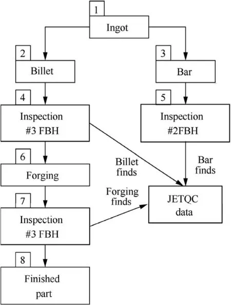
Fig. 1 Titanium component process model.

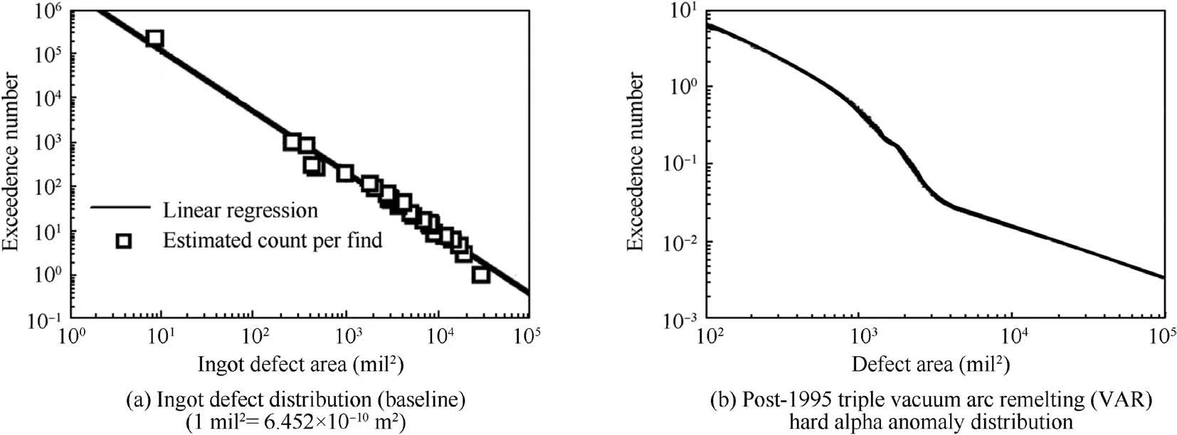
Fig. 2 Hard alpha anomaly distribution.32

Based on the experience from industry,this paper proposes an experimental method to obtain the hard alpha anomaly distribution for titanium alloy aeroengine disks that reflects and equivalently replaces the manufacturing development in titanium industry. The aim is to obtain the anomaly distribution in a relatively short period, and this anomaly distribution is associated with a specific country. This paper is divided into 6 sections. The generalization mechanism of the experiment is described in Section 2,including the definitions of the terms.Section 3 describes the experimental processes for TiN anomaly distribution,including the preparation of bulk TiN and the specimens,an anomaly detection probability experiment and a three-dimensional measurement experiment. Section 4 derives the anomaly distribution with the anomaly data and Probability of Detection (POD) data with several appropriate assumptions. Then, in Section 5, the probabilistic risk of a disk is calculated based on the anomaly distribution, and confidence intervals are introduced to evaluate the reliability of the results. Finally, the conclusions are summarized in Section 6.

2. Experimental methodology

The general programme for the experimental methodology,which aims at deriving the hard alpha anomaly distribution,is shown in this section. In general, the hard alpha anomaly distribution can be divided into two parts: the POD curve and the detected hard alpha distribution, which contains size and frequency data of detected anomalies.

2.1. POD curve

The POD curve is commonly represented as a function of the POD versus the flaw size, which is achieved using a specific Non-Destructive Equation (NDE) method, such as eddy current, penetrant fluid or ultrasonic method.Essentially, the POD curves are able to reflect and equivalently replace the detection capability in industry since they are dependent not only on the NDE method but also on a number of physical parameters (e.g. the materials, thickness of the component,flaw type, geometry). In this case, while the detection method,procedure and standard are specified and meet the actual industrial requirement, the POD curves can be obtained through repeated detection experiments. Regarding inherent hard alpha anomalies,ultrasonic detection is used mainly during the inspection period throughout the manufacturing processes of titanium components, including ingots, bars/billets and finished components. Therefore, in this paper, the POD curve of the hard alpha anomaly in titanium specimens can be obtained by this experimental method.

2.2. Detected hard alpha anomaly distribution

The detected hard alpha anomaly distribution contains the size and frequency of the anomalies.

Typically,the detected anomaly size data are collected from bars/ingots or finished components in production. Therefore,the size data are dependent on the remelting process for titanium alloy as well as the subsequent manufacturing processes.However,these size data are hard to collect because hard alpha(TiN) anomalies appear rarely in titanium high-energy rotors.In this case,TiN is artificially injected into titanium specimens,and acts as a surrogate for the natural anomalies.Notably,the titanium specimens with hard alpha anomalies should be manufactured through the same forging process as the actual titanium components to ensure that the deformation of the specimens is similar to that of the components.

Additionally, the frequency of the size data composes the cumulative distribution function, which depends on the randomness of the anomaly size.Generally, these detected anomaly size data fit a log-linear distribution in actual statistics.Moreover, the range of detected anomaly size data is dependent on the POD curve,which means that the minimum size is larger than the detection minimum threshold,while the maximum size is equal to the threshold size when the POD value reaches 100%. Therefore, referring to the log-linear distribution and the POD level,the distribution and size range of artificial TiN anomalies are initially determined. Certainly, the TiN continues deforming in subsequent manufacturing processes.Thus,the artificial hard alpha anomalies can be used as a surrogate for the natural anomalies by ensuring that the manufacturing processes are the same as the production processes and that the anomaly size range is similar to the natural situation.

On this basis,the details for the proposed method to determine the detected size distribution and the POD curve are shown in Fig.3.First,the hard alpha(TiN)anomalies are prepared, and a certain number of titanium specimens with/without anomalies are prepared in the laboratory and used for POD tests and size measurement.Second,the original detected hard alpha anomaly distribution from the specimens and the POD curve are derived.Third,to obtain the hard alpha anomaly baseline distribution, the detected anomaly distribution is corrected by the POD curve in conjunction with the manufacturing processes of a titanium rotating component from ingot conversion to inspected finished part. Finally, the hard alpha anomaly distribution of the finished part can be obtained combined with the actual anomaly information accumulated through production.

The hard alpha anomaly baseline distribution function Fis given by

where s is the crack sectional area;sis the minimum detectable crack area; p(s) is the probability density function of anomalies and p(s) is the POD of the anomaly with specific sectional area.

In short, the experimental method focuses on the laboratory preparation of hard alpha anomalies and bars/billets conforming to the manufacturing processes of titanium rotors instead of accumulating anomaly data in nature, as described by the FAA, for 3-5 years. In this way, the bars containing hard alpha anomalies can be obtained in a relatively short time rather than accumulating a sufficient amount of field data over a long time.

3. Experimental procedures

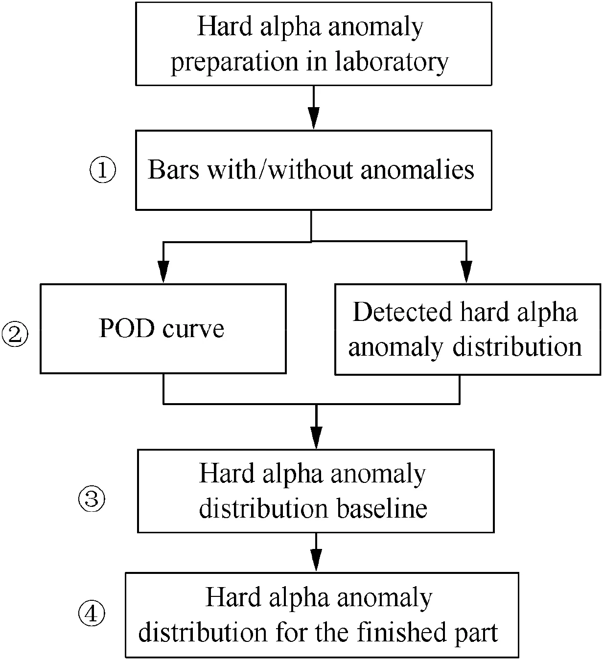
Fig. 3 Theoretical process for anomaly distribution characterization.

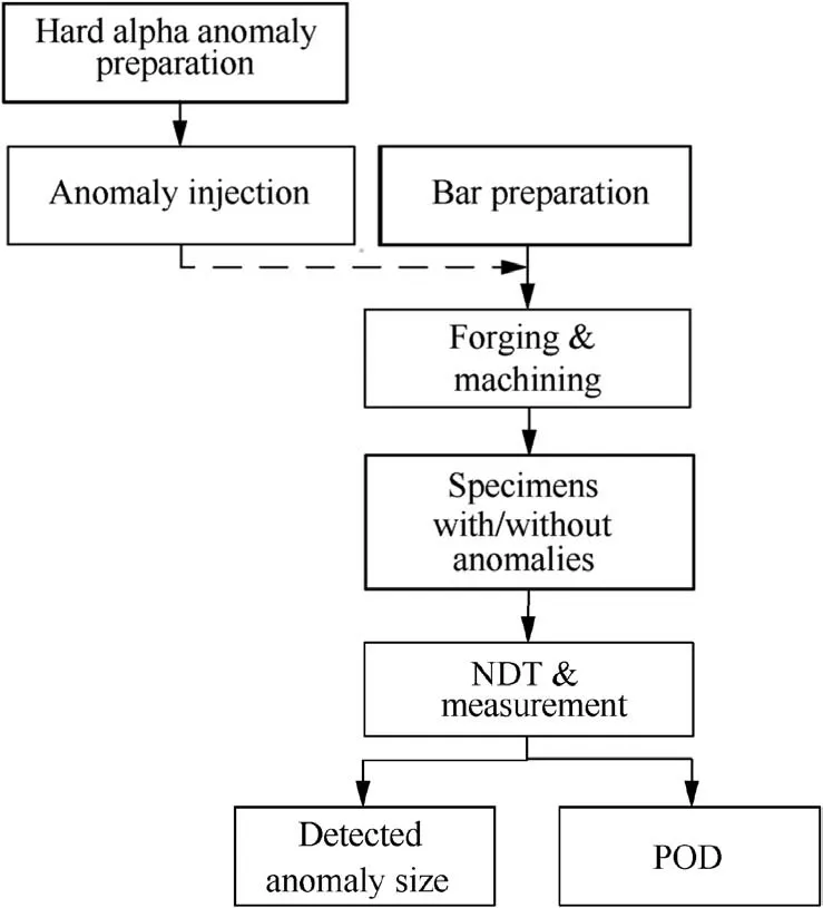
Fig. 4 Experimental scheme.

As shown in Fig. 4, the experimental method contains the preparation method for the hard alpha anomalies and the titanium specimens. In addition, the non-destructive test and anomaly measurement programme is introduced in this section to obtain the detected anomaly size data and the POD.

3.1. Hard alpha anomaly preparation

As mentioned above, hard alpha (TiN) anomalies are synthesized in an experimental method since natural anomalies are rare. The first task is to determine the weight ratio of N. The nominal nitrogen contents of the test specimens are 2%, 4%,6%,9%and 12%.In this paper,the nitrogen content is determined to be 12%since TiN with 12 wt.%N is relatively brittle, with a higher crack growth rate. Additionally, the crack growth validation tests reported by SwRIwere carried out with TiN with 12 wt.% N as the seed material. Hot pressing technology is an effective way to make artificial TiN materials with 12 wt.% N. An example of artificial TiN is shown in Fig.5.The processes are as follows:The titanium alloy powder and TiN(20%)are mixed in a certain proportion.Then,these components are transferred to the mould with a welding seal.Subsequently, the mould is placed in a Hot Isostatic Pressing(HIP)furnace with heat and pressure control.The composition analysis shows that the nitrogen content is 12.4%.

3.2. Specimen preparation

After the TiN is prepared, the titanium specimens (with/without TiN)are manufactured to obtain the POD data and defect size data of the interior anomalies. First, the standards of the specimens are presumed to meet the airworthiness requirements so that the POD test of the bar can be carried out and the artificial anomalies can simulate the defect through a real process. Based on the requirements of AC33.15-1,the converted material needs to have a cross-sectional area more than or equal to 16 square inches(10300 mm)and a width less than five times the thickness,implying that the diameter of the bar is greater than 4.52 inches (114.7 mm). In this case, the specimen standards are as follows: The material of the specimen is titanium alloy (TC4), and the specimen is manufactured to form a ∅4.72 inches×11.81 inches (∅120 mm×300 mm) bar which means that the diameter is 4.72 inches and the length is 11.81 inches.

Fig. 5 TiN made by hot pressing manufacturing technology.

The processes for manufacturing specimens with/without hard alpha inclusions are shown in Fig.6.The bar and anomalies are prepared, and then forged and machined. The specific steps for manufacturing the specimens are as follows.The titanium bars are manufactured, and the metal sponge and additional alloy, including pure aluminium and aluminiumvanadium alloy, are prepared. Then, the raw materials are mixed in a vacuum molten pool with a melting electrode. Triple Vacuum Arc Remelting (VAR) shown in Fig. 7(a) is utilized to prepare a titanium alloy ingot. The ingot is machined as a bar with ∅ 6.69 inches×5.9 inches (∅170 mm×150 mm). As shown in Fig. 7(b), 40 mm of the bar is removed due to porosity inclusions.

After that, anomaly injection is implemented. Certain round holes are machined in the end face of the ingots, and then titanium nitride anomalies of different sizes are inserted into the holes (Fig. 8), with each specimen implanted only one anomaly. Two ingots are welded together, and the anomaly-containing bars are processed hot pressing.

Melting is another way to obtain the specimen with anomalies by injecting TiN during the VAR process. However, melting has a poor effect since TiN material may break with the influence of thermo-mechanical stress and the diffusion of nitrogen makes TiN with 1.66 wt.% N, which is lower than 12.4% before the injecting process. Thus, hot pressing is an effective method to obtain specimen with anomalies.

In addition,the criterion for seed locations in the specimens is that the seeds must be in an inspectable(ultrasonic)location,have at least 0.1 inch effective strain and be in a widely dispersed pattern where adjacent seeds have no influence on each other.In addition,to carry out the POD test,half of the specimens are manufactured without anomalies under the same standard as the specimens with anomalies.

Subsequently, the forging(Fig. 9)and machining processes are carried out. Each forging process is divided into three steps. The ingot that has been processed with triple VAR is heated in a resistance furnace. The first forging temperature is T+(30-200)°C(1150°C),and the deformation parameter is ∅6.69-5.12-6.69-5.12 inches (∅ 170-130-170-130 mm),with a deformation quantity of 45%. The second heating is for the α+β phases: The heating temperature is T(30-60)°C (960°C), and the deformation parameter is ∅6.69-5.12-6.69-5.12 inches (∅170-130-170-130 mm), with a deformation quantity of 45%. The third heating temperature is 30-50°C below the β phase formation temperature.

Finally,the bar with anomalies can be obtained and is polished to remove the potential small cracks on the surface. In addition, the final component is machined with Ra ≥3.2 μm surface roughness as a ∅120 mm bar to meet the ultrasonic detection requirements (Fig. 10).

Another important aspect is how to choose the specimen number and TiN size. Since hard alpha anomalies are rare,the assumption is that the hard alpha inclusions in the specimens are distributed randomly, and each specimen contains only one inclusion.In the statistical description,the specimens are the samples, and their quantity is equal to the sample size.Intuitively,a large sample size is helpful for obtaining accurate POD curves(albeit with high cost),and the sample size can be combined with the confidence limit.To reduce the cost, the sample size can be minimized if the desired POD and confidence limit are first determined. The sample size n can be calculated by

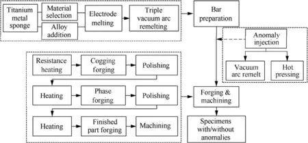
Fig. 6 Specimen manufacturing process.

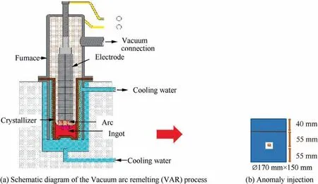
Fig. 7 3 VAR and anomaly injection process.

Fig. 8 Welded bars in anomaly injection process.

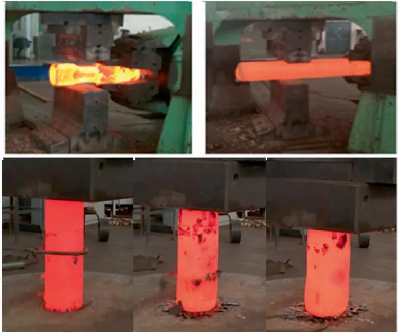
Fig. 9 Forging process.

Fig. 10 Geometry of bar specimens.

where Pis the proportion of samples containing the population, assuming that the total number of anomalies is the population; and 1-αis called the confidence level. The relationships among the sample size n, confidence level 1-αand subsample proportion Pare listed in Table 1.

In addition to statistical dependence,sample size n is dependent on the development of the manufacturing industry and the detection technique. Most anomalies larger than 4869.5 mil(2 mm) can be detected by ultrasound, while anomalies smaller than 194.8 mil(0.4 mm)can hardly be detected.Thus,the size range is preliminarily between 194.8-4869.5 mil(0.4-2 mm). Also, the differences in POD values among anomalies are very small when the size interval is less than 12.2 mil(diameter 0.1 mm). In this case, the preliminary size interval is 12.2-48.7 mil(0.1-0.2 mm). Thus, the sample size n is set as 8,which means that 8 flaw-inclusive specimens were manufactured. In order to conduct the POD research. another 8 flawexclusive specimens were manufactured. The subsample proportion is approximately 80%,with 50%confidence according to Table 1.

In conclusion, the initial sizes of the artificial TiN specimens are ∅19.7 mil×19.7 mil, ∅35.4 mil×35.4 mil, ∅47.2 mil×47.2 mil, and ∅ 59.1 mil×59.1 mil (∅0.5 mm×0.5 mm,∅0.9 mm×0.9 mm,∅1.2 mm×1.2 mm,and ∅1.5 mm×1.5 mm). During the forging process, the deformation of the TiN results in a size change.

3.3. NDT and measurement standards

The NDT standards refer to MIL-STD-2154.As mentioned in airworthiness advisory circular 33.14-1,the POD curve used is the mean POD for ultrasonic inspection of field components,with reject indications equal to or greater than those from a 3/64 inch(1.19 mm)diameter Flat Bottom Hole(FBH).In this experiment,the detection level is AA,which complies with the airworthiness requirements.

The ultrasonic NDT is divided into two types: manual detection and automatic detection (Fig. 11). Human factorsalso affect the anomaly detection probability. The automatic detection method is an advanced inspection technology commonly used in titanium bars with high accuracy and stability.Five different probes and methods are used in this experiment(Fig.12).The total number of detections is 50,as illustrated in the following demonstration. More than 5 inspectors are involved.Each of them conducts ultrasonic detection independently without sharing information with others. For the same specimen, each inspector needs to conduct detection no more than once a day.

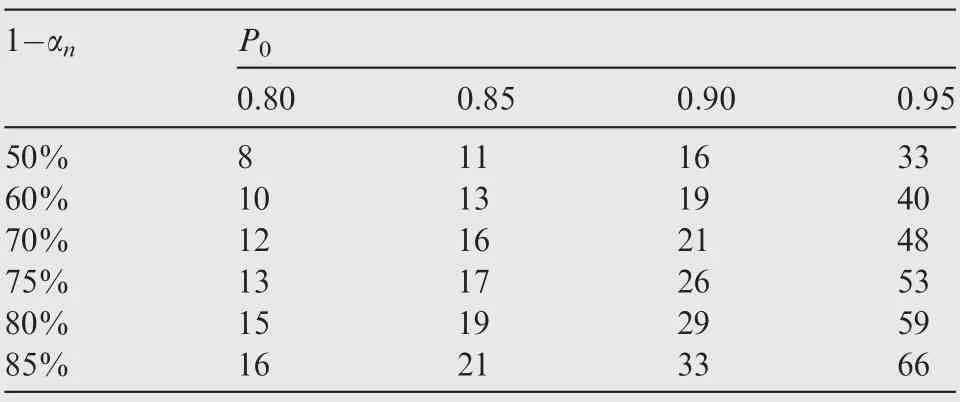
Table 1 Relationships among n, 1-αn and P0.

The mean value of probability of detection ^pcan be obtained by

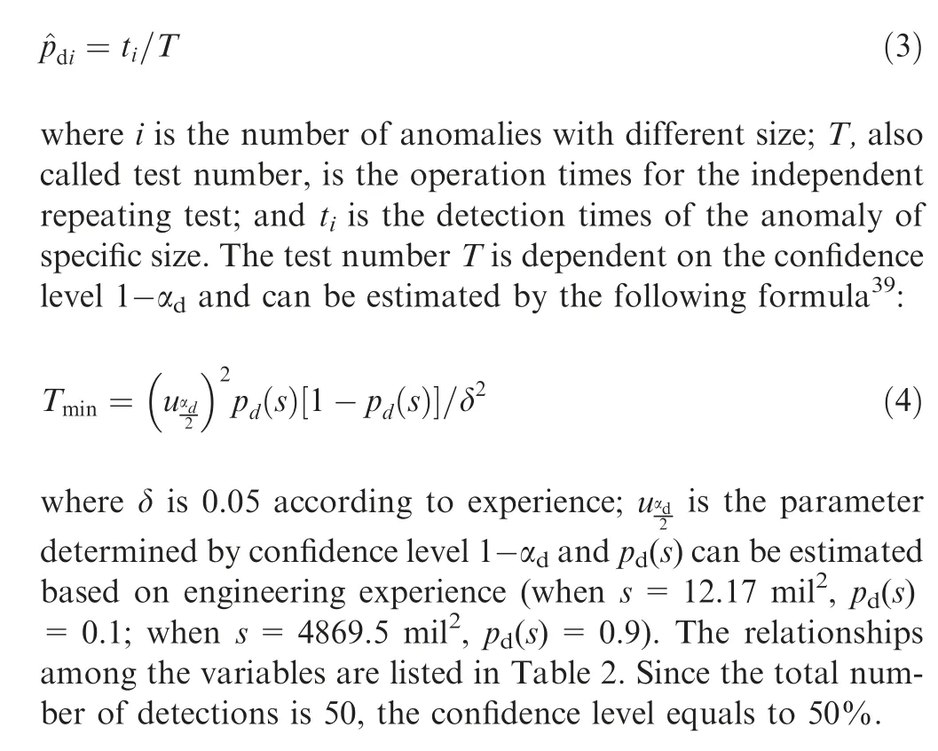
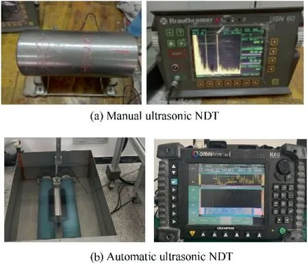
Fig. 11 Ultrasonic NDT of bar.

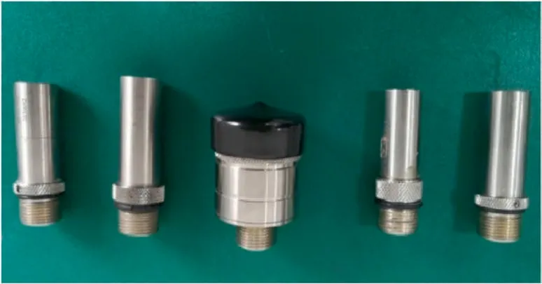
Fig. 12 Ultrasonic NDT probes.

Finally, the three-dimensional sizes of the anomalies were obtained through Computed Tomography (CT) and metallographic analysis. The specific process is shown in Fig. 13.

First, the specimens are scanned by CT to localize the anomaly. Then, the specimen is cut as a ∅0.787 inch×0.59 inch(∅20 mm×15 mm)cylinder with an anomaly at the centre point by Wire Electrical Discharge Machining (WEDM).Second, the cylinder is polished and subjected to detection.Third,the cylinder is gritted with waterproof sandpaper of different grit numbers to expose the defect (Fig. 14). Finally, the metallographic samples are analysed by Scanning Electron Microscopy (SEM).

3.4. Anomaly size and POD data

In this experimental programme, 16 specimens with 8 anomaly-containing specimens are subjected to detection at least 50 times for each POD value. The compositions and three-dimensional sizes of the anomalies are obtained through metallographic sectioning or CT mentioned above.

Finally,the three-dimensional sizes and detection probability data of the TiN with 12 wt.% N are obtained shown in Table 3. A, R and C represent the axial, radial and circumference sizes respectively (Fig. 15). The TiN sectional area sin the bar can be calculated by Eq. (5) in Section 4.1. The TiN area ranges from 1000 milto 2500 milwith the deformation induced by forging and other heat treatments.

4. Results and discussion

This section derives the anomaly distribution with the detected anomaly size and POD data obtained through the experimental process mentioned above. Several assumptions are proposed to obtain the most appropriate anomaly distribution.The specific steps are shown in Fig.16,where the original distribution of detected flaws is corrected by the POD curve in combination with the manufacturing processes of a titanium rotating component from ingot conversion to forging inspection.

4.1. Results of the POD curves

POD curve can be derived from the anomaly size and the detection data in Table 3.The cross-sectional area of the defect in the bar perpendicular to the detection direction scan be calculated by the following formula:

Table 2 Minimum detection times.

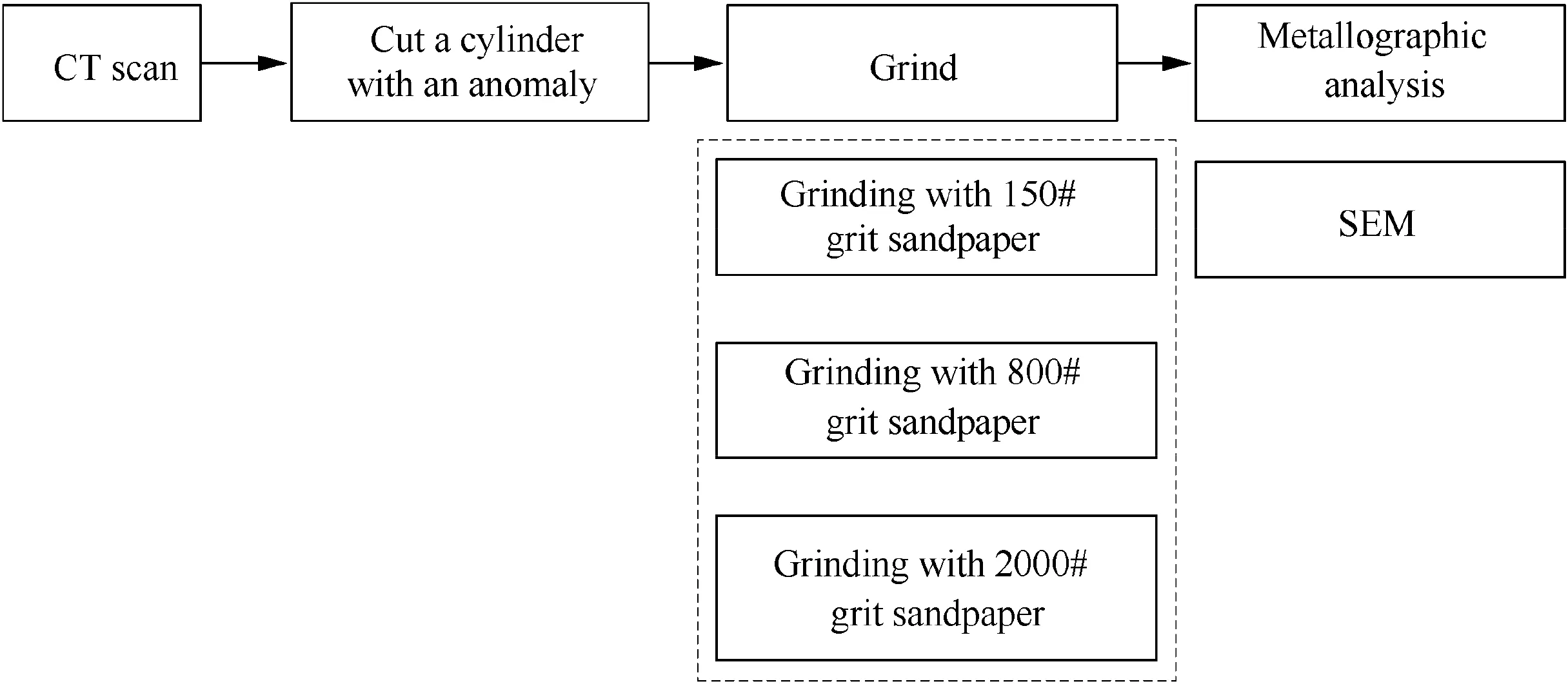
Fig. 13 Metallographic analysis process.

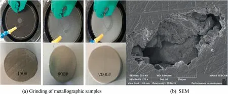
Fig. 14 Grinding of metallographic samples (different sandpapers) and microstructure of an anomaly.

Table 3 Anomaly size and POD data sheet.

where A is the axial size, R is the radial size and C is the circumference size, as shown in Fig. 15.

The binominal distribution arises when units are classified into two groups:defective and non-defective.The probability value can be obtained through independent binomial experiments and given by

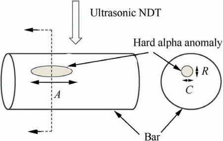
Fig. 15 Ultrasonic NDE test of a hard alpha anomaly.

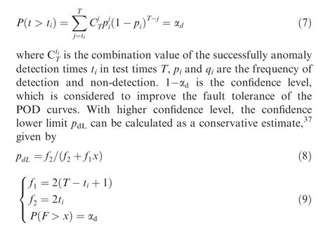
where fand fare respectively the first and second degrees of freedom of the F distribution, x is the upper quantile of the F distribution, which is the operation times for the independent repeating tests.

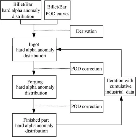
Fig. 16 Iteration through component processes.

where sis the cross-sectional area of anomalies in the bar considering the defomation caused by forging process; η and β are the scale parameter and shape parameter in Weibull distribution respectively, and pis the probability of detection.The Weibull parameters for mean POD value is η=2412.76，β=1.11817.

Fig.17 is the POD for ultrasonic inspection of field components with #2 FBH calibration. The POD curve with a 50%confidence level is close to the mean point estimate data, and the Root Mean Squared Error(RMSE)value is 0.0021,which means that the point estimate has a 50% confidence level.

This result indicates that the sample size of the POD test is 50 for each anomaly. In addition, the confidence level is the same as that of the default POD curves supplied in AC33.14-1. Nevertheless, there is a larger difference between the mean value and other POD curves with higher confidence levels since the NDT measurement number is less than required. This result means that the higher confidence level corresponds to a larger detection number. However, since the detection number is limited by the experimental cost, the POD lower limit data with a higher confidence level are calculated by statistical method as a conservative estimate, which is lower than the experimental mean value.

4.2. Results of the hard alpha anomaly distribution

The ingot hard alpha anomaly distribution is derived from the actual size data and POD of the bar. Two assumptions are proposed: (A) the anomalies in the bar originate from the initial ingot, and the number of anomalies remains constant. (B)The volumes of the hard alpha anomalies in the ingot remain constant as the anomalies transform from a sphere to an ellipsoid.In addition,an elongation modelis assumed to describe the change in the anomaly shape.

The number and size of the anomalies are described by the following expressions

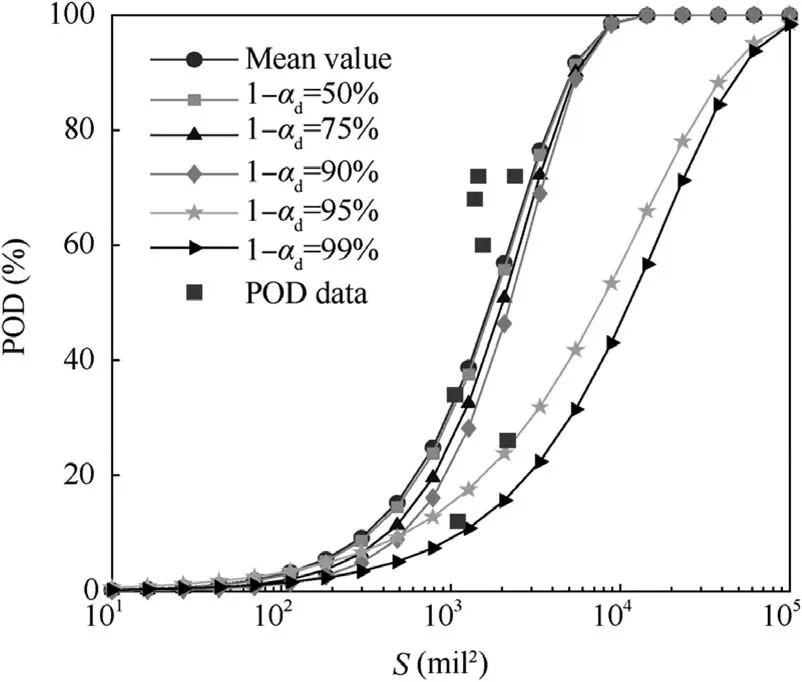
Fig. 17 Experimental POD curves with different confidence levels.

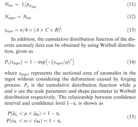
With the anomaly size data and anomaly number data,the anomaly distribution in the ingot is obtained (Fig. 18) by the log-linear fitting method through the third assumption: (3)the size data and the anomaly number have a log-linear relationship.

where Fis the number of anomalies larger than a specific sectional area S; Nand kare the intercept and slope of a linear function respectively. S=ssince the sectional area of the anomalies is calculated with Eq. (13) to obtain the anomaly size in the ingot.

Then,the bar anomaly distribution is obtained by the translation of the ingot baseline (Fig. 19). In this case, S=s.Based on the hard-alpha anomaly elongation model, the area of the bar anomaly is calculated.

Subsequently, with the baseline of the ingot titanium part,the distribution of the finished part can be derived based on the process model including the POD data (Fig. 20). An additional three assumptions are put forward: (A) the section size of the TiN remains unchanged from bar to forging, as the radius changes only minimally. (B) The POD curve applied to the bar component is assumed to be suitable for other components,including the billet,forging part and finished part.In addition, the maximum POD is assumed to be 80% rather than 100% based on industrial experience that the POD cannot reach 100%even when the anomaly size is relatively large.(C) Experience in the context of American industry indicates that the detection rates of anomalies in bars and billets are no more than 1 and 0.6 finds/million pounds, respectively.

The anomaly distribution of finished part is derived under the assumptions mentioned above, as shown in Fig. 20.

4.3. Comparison and analysis

To analyse the precision of experiments,the results of the POD and anomaly distribution are compared with the reference curves from AC33.14-1 and relevant reports.

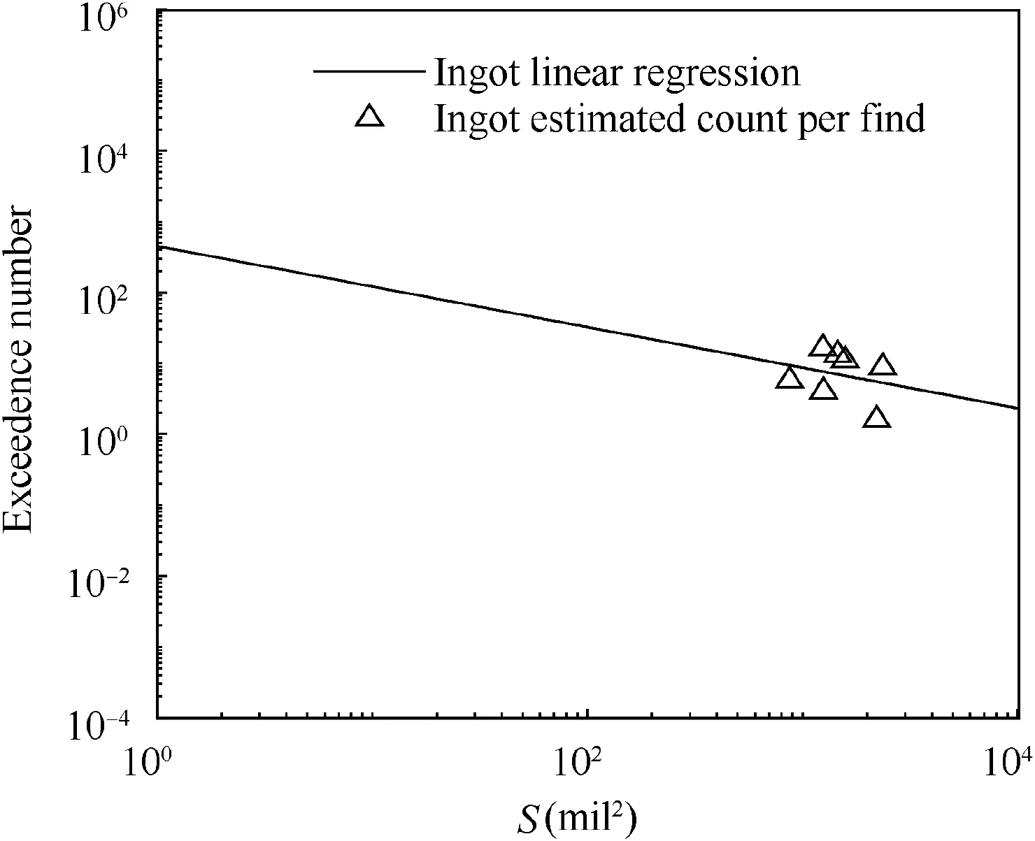
Fig. 18 Ingot baseline.

Regarding the POD curve, the experimental result differs from the default reference curve under the same detection conditions.Fig.21 is the mean(1-α=50%)POD for ultrasonic inspection of field components, which shows that the experimental POD curve is higher than the default curve, which means that the POD level has improved during the past 2 decades.

Regarding the detected anomaly size,the size data collected over 3-5 years from the report are much higher than the artificial data in this paper. Since the detectability is lower in that time, more anomalies with larger sizes are recorded. In addition, few minor defects hard to be detected are recorded by chance. Fig. 22 shows the difference between the detected size data and derived ingot baseline. The experimental ingot baseline is flatter since the size data range is limited without small anomalies. Fig. 23 shows the final anomaly distribution derived from the size data and the POD data with appropriate assumptions and titanium component processing. The experimental anomaly size distribution has a lower slope (the slope value is larger), which means that fewer small but more large anomalies exist.

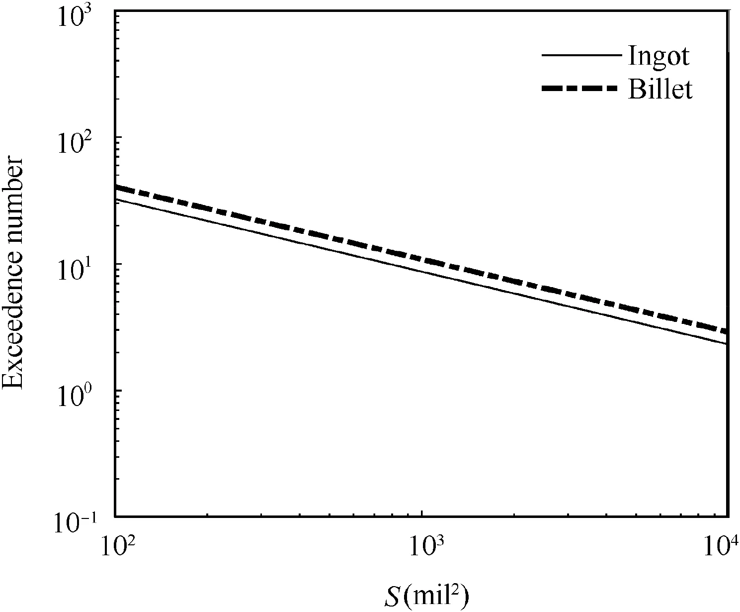
Fig. 19 Bar baseline.

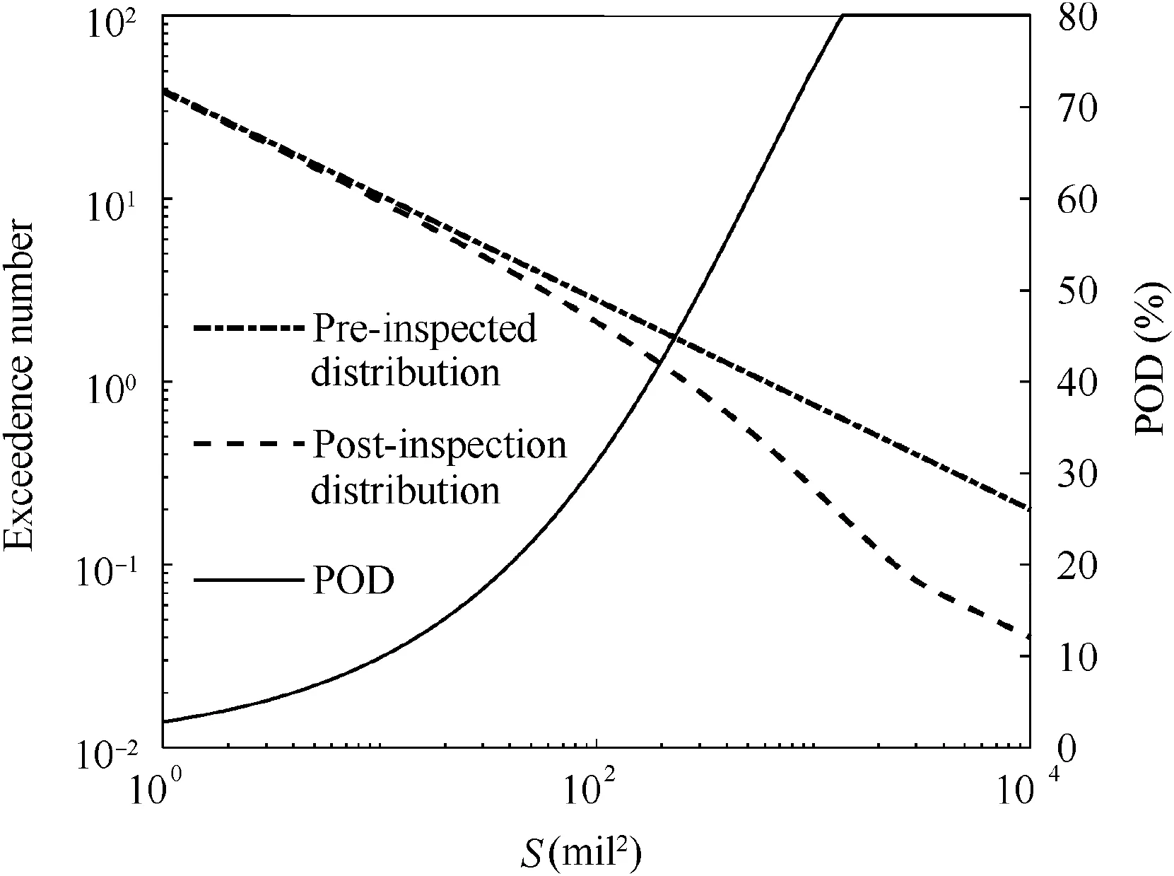
Fig. 20 Finished part distribution.

Nevertheless, the artificial anomalies cannot entirely represent the actual anomalies. The materials removed by inspection from the in-process material should be collected and processed into metallographic sections to acquire the industrial cumulative data. The anomaly distribution should be updated with the development of manufacturing technology. With more minor defect data, the distribution curve will be steeper.On this basis, the slope is the critical parameter to reflect the proportion of the minor and large defects.

5. Sensitivity analysis of the probability of failure (POF)

This section calculates the POF of a rotor disk with the derived anomaly distributions as the critical input data,which is determined by the POD curves and detected anomaly size data.Generally, the POD curve is also influenced by the confidence level, and the difference in the anomaly size data is quantified with the slope of the exceedance baseline, which is used to derive the final anomaly distribution. In this section, the confidence level of the POD and the slope of the baseline are considered important variables that affect the anomaly distribution curves and the POF.

5.1. Assessment framework and mechanical analysis

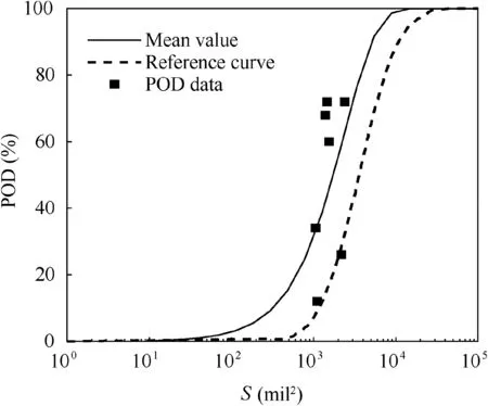
Fig. 21 Experimental and AC default POD curves.

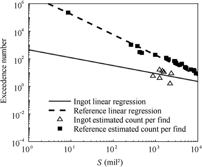
Fig. 22 Experimental and reference ingot baseline.

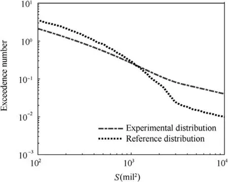
Fig. 23 Experimental and reference finished part distribution.

The POF of a rotor disk is calculated through operating cycles based on the probabilistic damage tolerance method.This methodology integrates FE stress analysis results, fracturemechanics-based life assessment for low-cycle fatigue and inspection schedules to determine the POF; the basic process is shown in Fig. 24. The equivalent stress and crack growth laws are important for calculating the POF.The POD curve and anomaly distribution are essential for life assessment analysis.

The 3-D FE model is a type of titanium compressor disk,as shown in Fig.25. ˙m is the inlet mass flow rate,Tand Tare inlet and outlet temperature, Pis outlet pressure o and N is the rotating speed. The material for the test case rotor is Ti-6-Al-4-V. The physical properties are provided in AC 70-1. The boundary conditions are typical compressor operating conditions as listed in Table 4.

With the FE model and the typical boundary condition,the principle stress can be obtained and the stress counter is shown in Fig. 26(a). Linear elastic fracture mechanics analysis is the core part of the probabilistic damage tolerance methodology and can be used to calculate the Stress Intensity Factor(SIF), which is the characterizing parameter of the crack tip stress-strain fields and the crack driving force.The Paris model and the weight function empirical equations are used in the crack growth calculation.

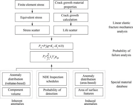
Fig. 24 General probabilistic framework for risk prediction of components with anomalies.

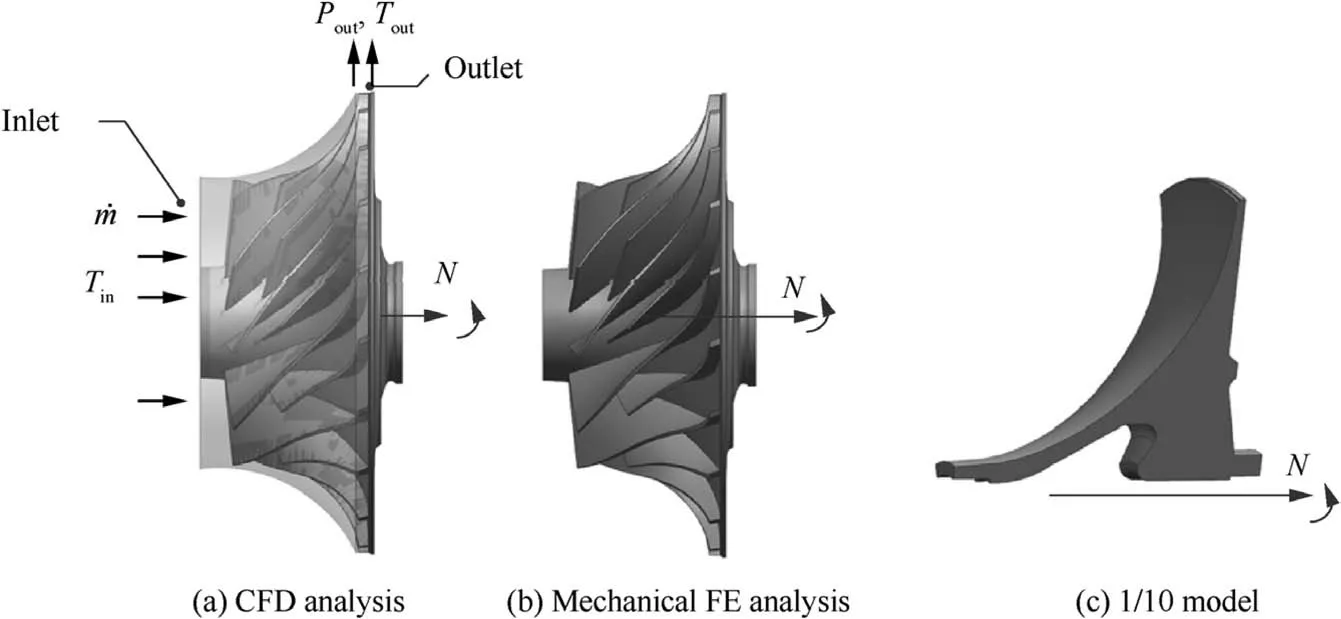
Fig. 25 3-D geometry UG model of compressor disk.

Table 4 Boundary condition lists.

POF analysis is conducted based on stress strength interference theory. The limit state function,which can be determined by comparing the fracture toughness with the SIFs, is the physical description of stress strength interference theory.TiN anomaly is an inherent anomaly which can be located anywhere within a component.The components can be subdivided into a manageable number of zones (Fig. 26(b)) of approximately equal risk to account for the uncertainty in the location. Zone-based methodologyis used to calculate the POF and the POF in each zone pcan be obtained by

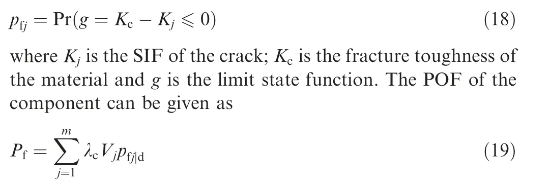
where pis the zone POF under the condition that a defect exists in zone j;λis the anomaly occurrence rate per unit volume of a component and Vis the volume of the zone j.

5.2. POF influenced by POD curves

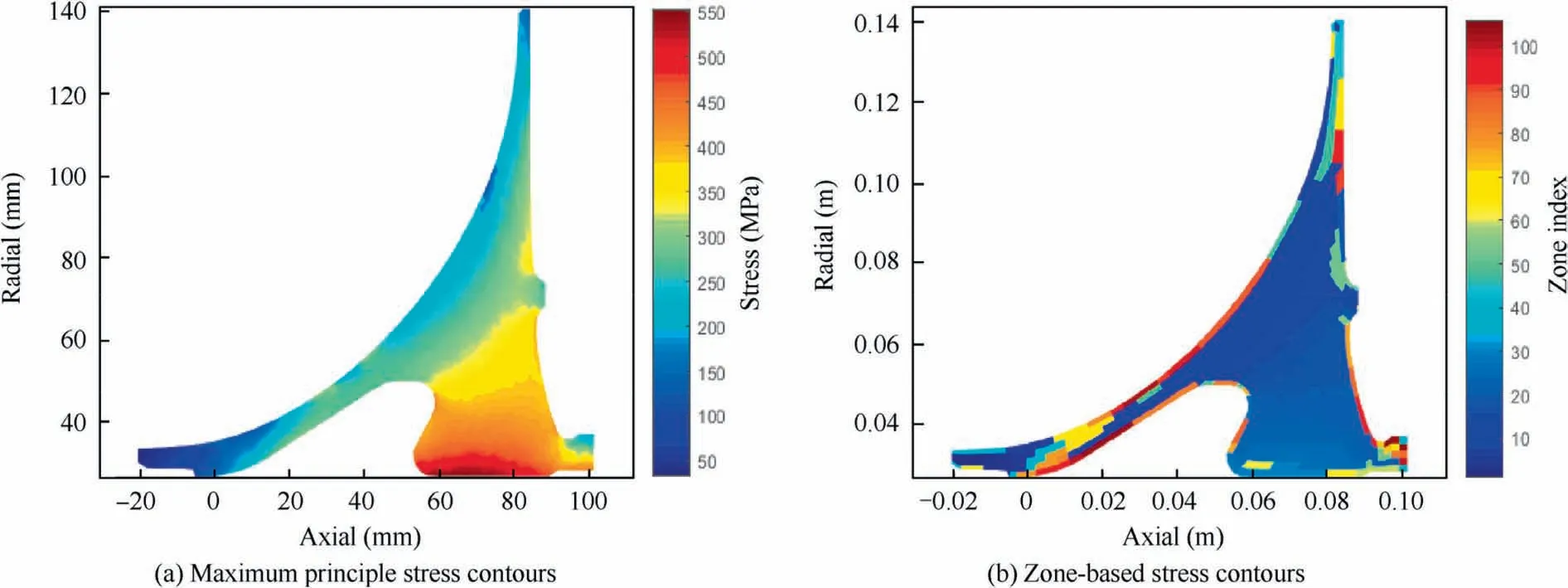
Fig. 26 Maximum principal stress at maximum loading.

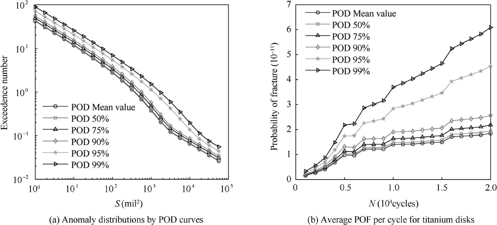
Fig. 27 Anomaly distribution and POF with different POD curves.

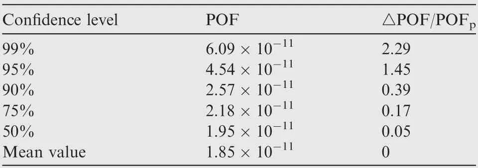
Table 5 POFs with different confidence levels for POD curves.

The anomaly distributions influenced by different POD curves with different confidence levels 1-αcan be derived.With the consideration of the confidence level 1-α, the confidence lower limit can be calculated to improve the fault tolerance(Fig.17).The anomaly distributions with different POD curves with a 50%-99% confidence level are derived based on the assumption that the detected rates of anomalies in bars are less than 1 find/million pounds.The final anomaly distributions are shown in Fig. 27(a).

With the equivalent stress distribution, the probabilistic assessments are used for titanium disks, and the results are shown in Fig.27(b).According to the specific POF data listed in Table 5, the POD mean value and 50% confidence level have similar POF values, which proves that the POD mean value has a 50% confidence level. In addition, a POD confidence level greater than 90% results in higher POF values.In this case, a security coefficient should be considered if the confidence level improves. In all, the 50% confidence level can meet the airworthiness requirements.

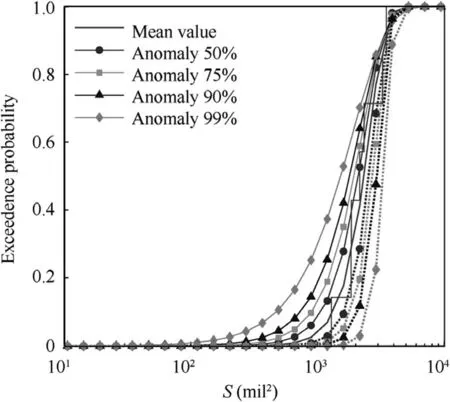
Fig. 28 Detected cumulative distributions with different confidence level.

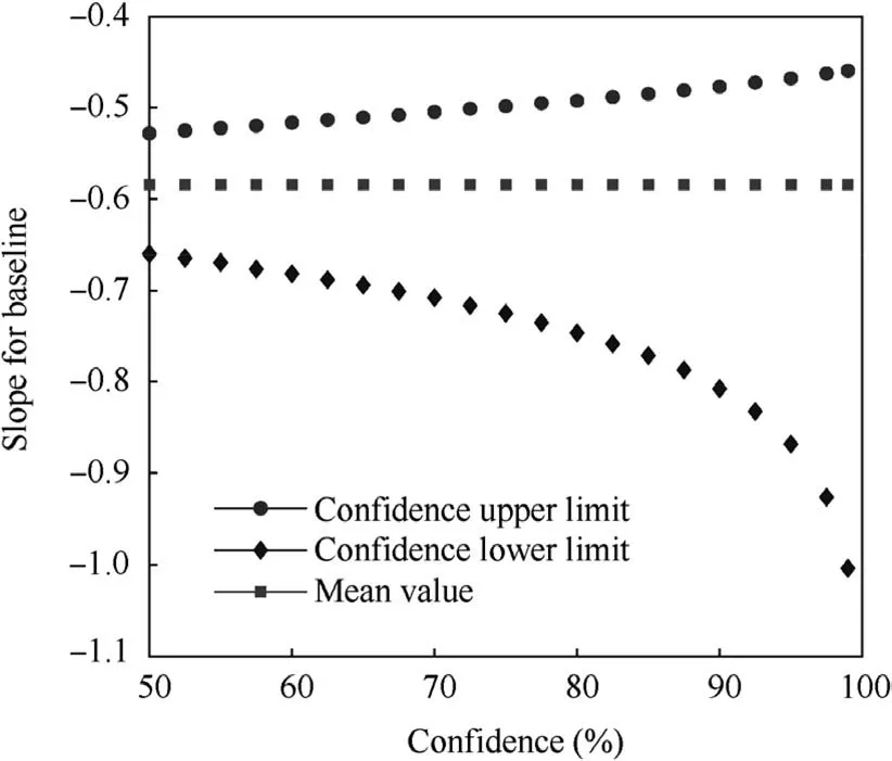
Fig. 29 Derived anomaly slope data.

Based on the analysis, it is clear that a higher POD confidence level corresponds to a smaller POD value. Meanwhile,the POD value has a 50% confidence level when the test sample size is 50. The anomaly distribution is associated with the POD curves,and the higher the POD is,the lower the anomaly distribution is. The POF value is also determined by the POD curves, and a coefficient is proposed to be used when the confidence level becomes higher in Table 5.

5.3. Anomaly distribution influenced by size data

The detected size data are also necessary for the derivation of the anomaly distribution.The discrete size data are normalized as a cumulative distribution, where the horizontal axis represents the anomaly size, while the vertical axis represents the cumulative probability from 0 to 1. Fig. 28 shows the column diagram of the cumulative distribution,and a Weibull curve is used to fit the cumulative distribution. Different size data dis-tributions can be obtained by changing the confidence level 1-αof the fitting Weibull curve.

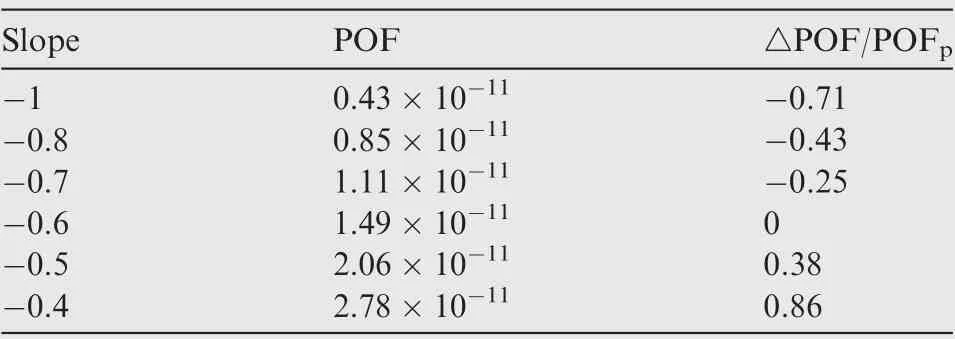
Table 6 POFs with different baseline slopes.

Then,the exceedance baseline can be derived with different Weibull curves. Generally, the baseline can be fitted with the log-linear function, and the slope of the baseline is the critical factor to quantify the randomness of the size data. Fig. 29 shows the slope data of different Weibull curves with different confidence levels 1-α, the slope of the baseline ranges from-1 to-0.45.For the upper confidence limit,the slope is larger and the curve is flatter,while for the lower confidence limit,the slope is smaller and the curve is deeper.

The final anomaly distribution with different slopes is shown in Fig. 30, and the POF is calculated. The slope of the curve has a positive relationship with the POF.In addition,a multiplicative correction factor is applied to the POF in order to obtain the conservative estimate.

Based on the analysis, the slope of the baseline reflects the difference between the detected size data. The larger the slope value is, the higher the POF is since the anomaly distribution tends to be flatter. The coefficient should be considered when the confidence level becomes higher with reference to Table 6.Note that the detected anomaly data should be accumulated through the real production process. Based on experience of the American titanium industry, the detected anomaly distribution tends to be steeper with additional small anomalies,and the slope tends to be smaller(approximately-0.8).In this case,the POF decreases since there are more small cracks and fewer large cracks.

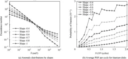
Fig. 30 Anomaly distributions and POFs with different baseline slopes.

6. Conclusions

An experimental methodology for obtaining the hard alpha anomaly distribution,which is the key input to the probabilistic risk assessment methodology in a relatively short term with data from the laboratory,is presented in this paper.The anomaly distribution can be established based on several appropriate assumptions, and the probabilistic risk of a disk is calculated with the anomaly distribution to evaluate the reliability of the results.Some general conclusions of this study are as follows:

(1) The experimental method aims to obtain artificial hard alpha anomalies that can serve as a surrogate for natural anomalies when a reasonable size range is chosen. The TiN size range is 194.8-4869.5 mil(diameter 0.4-2.0 mm), and the size interval is approximately 109.6-194.8 mil(0.3-0.4 mm). In this case, the number of flaw-inclusive specimen is approximately 8-16. This experimental method can preliminarily obtain the anomaly distribution, and the POF can be calculated.

(2) The anomaly distribution is dependent on the POD and the anomaly size data, which are associated with the confidence level.In terms of the POD curves,the higher the POD is, the lower the anomaly distribution is. The POF with the mean POD curve is 1.85×10, while the POF with the 50% confidence POD is 1.95×10,and the relative error is 0.5%.The conservative POF can be obtained by increasing the confidence level.

(3) Regarding the anomaly size data, the cumulative curves reflect the distribution of size data with different confidence levels. Furthermore, different cumulative curves correspond to different slopes of the exceedance baseline.The larger the slope is,the higher the POF is,since the distribution tends to be flatter.The slope of the baseline ranges from -1 to -0.45 with a 99% confidence level.When the confidence level is 50%,the slope ranges from -0.65 to -0.52, and the POF ranges from 1.4×10to 2.0×10. In this case, 2.0×10can be considered the conservative estimate.

Notably, actual hard alpha anomaly data should be accumulated, with the most important data being the anomaly finds/million pounds and the detected anomaly size.The distribution will be updated and modified by the data collected through manufacturing.With more minor defect data,the distribution curve will be steeper, and therefore the probabilistic risk can be expected to be decrease in the future.

Declaration of Competing Interest

The authors declare that they have no known competing financial interests or personal relationships that could have appeared to influence the work reported in this paper.

Acknowledgement

s

The work was funded by the National Natural Science Foundation of China and Civil Aviation Administration of China(No. U1833109). The work was supported by the Innovation Team of Complex System Safety and Airworthiness of Aero Engine from the Co-Innovation Center for Advanced Aeroengine of China.