Development cost prediction of general aviation aircraft using combined estimation technique

Xiaonan CHEN, Jun HUANG, Mingxu YI

School of Aeronautic Science and Engineering, Beihang University, Beijing 100083, China

KEYWORDS Combined prediction method;General aviation aircraft;Optimal weight;Shortest ideal point method

Abstract Obtaining accurate development cost estimation results of general aviation aircraft is crucial for companies to adopt the best strategy in the development process. To address this problem, this paper proposes a combination of three commonly used single prediction methods. The optimal weight values of the three single prediction methods are determined by utilizing the shortest ideal point method.Ten cost datasets collected from literature are utilized for fitting and testing the combined prediction method,and the weight coefficients of the three individual prediction methods are calculated as 0.6859, 0.0035 and 0.3106, respectively.The results of this study indicate that the developed method has better fitting and estimation accuracy than that of the three individual methods, with average fitting and predicting error values of 2.60% and 6.43%, respectively. Additionally, the cost data of military and civil aircraft development from literature are collected for verification.The results further confirm that the proposed method is not only superior to the single prediction methods in terms of high precision but has wider applications. More importantly, this research can provide important reference for general aviation aircraft companies in term of product cost planning and corporate sales strategies.

1. Introduction

An accurate development cost estimation method for quick formulation of reasonable product sales prices is extremely important for decision-making and competitiveness improvement of companies.However,the gap between the availability of large numbers of general aviation aircraft and relatively scarce cost data is not expected to narrow in the short term owing to the difficulty in data collection, lack of relevant parameter information,company confidentiality,and the short development time.Over the past few decades,numerous parametric prediction methods have been developed to obtain accurate cost prediction results.

The single prediction methodology is the most popular parametric prediction method.Among all the single prediction methods, the most commonly used include the method of Partial Least Squares Regression (PLSR) that can be utilized in cases of small sample size, the Back-Propagation(BP) method that is used to fit the model well based on the deep learning ability, and the Stepwise Regression (SR)method which is employed to reduce the number of variables for model simplification. The PLSR method is suitable for cases with limited sample number, high correlation between variables and large data loss.For example, Li and Songdeveloped a prediction model using the PLSR method to predict the cost of fuselage development. Despite the popularity and usefulness of the PLSR method in many cost prediction problems, some drawbacks exist. For example, as proposed by Wu et al.,it is not suitable for systems with a large number of complex variables, since the multi-collinearity among the variables will lead to deviations in the interpretation of the results.In recent years,researchers have tried to overcome the disadvantage of the PLSR method by utilizing neural network systems, because this method can better deal with the problems of multi-collinearity data. Curran et al.employed a BP method to predict the aerospace engineering cost. Yao et al.developed a BP model to forecast tourist arrival and tourist demands.The analyses results show that the intelligent prediction methods are useful and effective. Gu¨naydın and Dogˇanutilized the BP method to estimate the building cost.However, they obtained poor prediction results when data were limited.The SR method is probably one of the most commonly used research practices in substantive and effectiveness studies. Zhou et al.presented an SR model to estimate dominant modes, proving the effectiveness of the developed method. Tahmasebi et al.used the SR method to estimate the target parameters and observed that inaccurate predictions are a result of data insufficiency.Meanwhile,highly correlated independent variables may lead to an unreasonable optimal subset.

Due to the inherent defects of single prediction methods,the above-mentioned approaches cannot always provide satisfactory prediction results. As prediction-associated problems are usually complicated in reality and the data samples are small, single prediction methods are not mutually exclusive;instead, they have complementary relationships.For prediction problems, the common way is to establish several different single prediction models, and then choose the one with the best prediction accuracy. This practice only selects the most suitable prediction model for different data instead of substantially improving the prediction accuracy. Therefore,for the purpose of a more accurate prediction performance,combined prediction methods have been developed. Sonmez and Ontepelicombined the regression method with a BP neural network method to estimate urban railway costs, with results indicating that a relatively accurate estimation behavior can be obtained by the combined method.Liu and Xiecombined a BP method with the GM (0, N) method to solve the problem of civil aircraft cost estimation, indicating that the combined prediction method can achieve the ideal prediction effect.

Despite the increasing utilization of the combined prediction method,research on the general aviation aircraft development cost still remains scant. Based on the characteristics of the PLSR, BP and SR methods, this study will apply a combined method to the prediction of the general aviation aircraft development cost. The rest of this paper is organized as follows. Section 2 introduces three single prediction methods,namely, PLSR, BP and SR. The combined prediction method is then introduced in Section 3,which also discusses the shortest ideal point method for obtaining the optimal weight of the combined prediction method. Section 4 presents case studies using collected cost data, to which the three single prediction models and the combined prediction model are applied. The fitting and prediction results are summarized, and the feasibility of combined method determined in Section 5. Finally,concluding remarks and future work are presented in Section 6.

2. Single prediction models

2.1. PLSR method

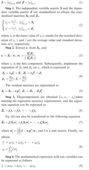
Assume that the independent variable swith h samples are expressed as a matrix S, while the dependent variable z with h samples are expressed as a matrix Z.

2.2. BP method

The Artificial Neural Network (ANN) is an abstract mathematical approach with non-linear processing, self-adaptation,and self-learning capabilities. Among all the neural networks,BP method is the most commonly used one. A typical BP model contains three interrelated layers,namely,input,output and hidden layers. In addition, each layer has its own initial weight, number of neurons, function of neurons and biases.Summation and activation are the two functions performed by neurons on each layer.Fig.1 shows the typical architecture of a BP model.The detailed description of each phase has been introduced in our previous work.

2.3. SR method

The stepwise regression method is used to individually introduce parameters into the model. After that, the model is subjected to an F test. If the initial interpretation parameter is no longer significant after the introduction of the subsequent explanatory variable, it is eliminated. This process is repeated until no significant explanatory parameters can be introduced into the regression model.

Step 1. Assume that there are u independent variables and one dependent variable; the correlation coefficient matrix R between all the variables can be expressed as

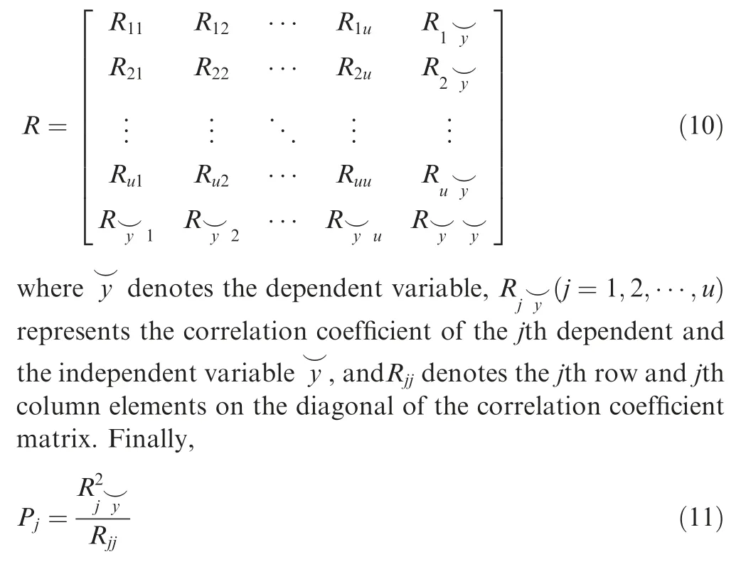
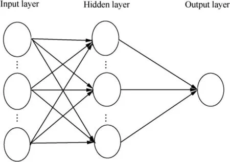
Fig. 1 Architecture of BP model.

where Prepresents the contribution of the coefficient of the jth independent parameter to the dependent parameter. Subsequently, the contribution coefficient calculated in step l is

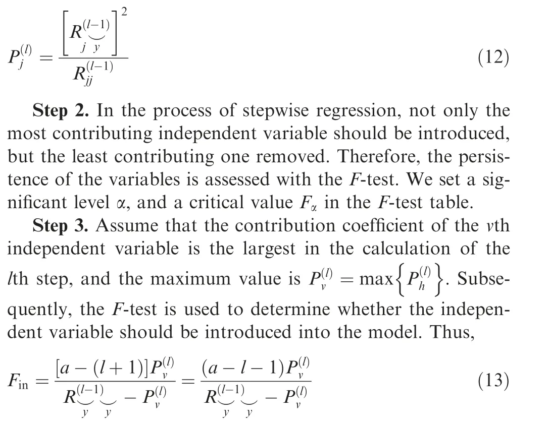
where a represents the sample number,v(v=1，2，···，u) is the serial number of the original variable corresponding to the selected variable, and the value of F introduced by the variables is represented by F. If F＜F, the variable can be introduced into the model. Otherwise, it is not introduced.

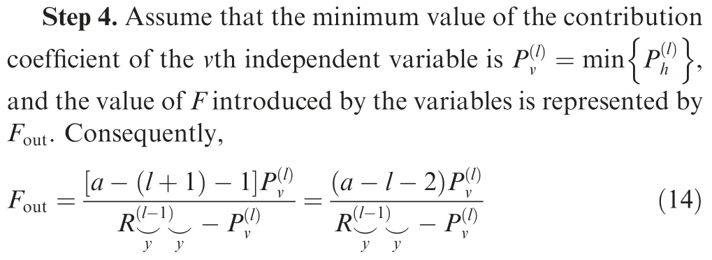
If F≤F, then the variable should be removed at this level of significance.

Step 5.Repeat Steps 3 and 4 until all the necessary variables have been introduced, and the inessential ones removed.

3. Combined prediction method

The result of the combined prediction method can be described as

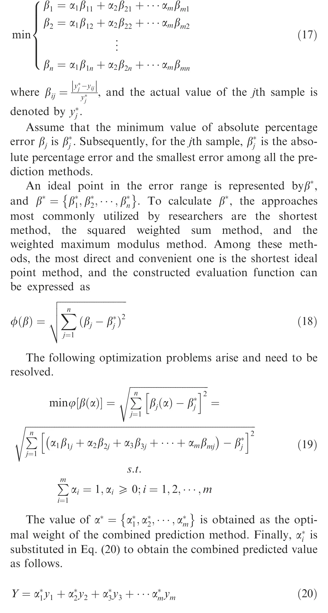
where Y is the result of the combined prediction,α(i=1，2，···，m) the weight coefficients of each single prediction method,and y(i=1，2，···，m)the result of the single prediction method.

The key factor determining the result of Y value is the weight coefficient α, which can be determined by the linear weighted sum method, square sum weighted method, evaluation function method,ideal point method,and other methods.Among these methods, the ideal point method has its solution advantage because of its short calculation time, reasonable structure, relatively simple principle, and high resolution.

The ideal point method is a multi-objective comprehensive evaluation method to rank the relative merits of a finite number of evaluation objects according to their proximity to the ideal object, and the predicted result can be expressed as

The optimal weight coefficient αin the combined prediction method can be determined by minimizing the absolute percentage error, the mean absolute percentage error, the squared error, and the absolute error. In this study, the absolute percentage error βminimization is selected as the goal of optimizing the weight coefficients, with one of the major reasons being that the absolute percentage error can be utilized as the criterion to determine the prediction results.

4. Case studies

4.1. Parameter description

Case 1. Data on ten general aviation aircraft projects were collected from the book by Qu.Fig. 2 shows the product drawing of a general aviation aircraft project. Six projects are randomly selected as training samples for each single prediction method,while the seventh and eighth samples are used as benchmark samples to implement the combined prediction model. The ninth and tenth samples are utilized as the test samples.

Not all of the design parameters have a positive or significant impact on development costs. Cost-driven factors can be obtained by retaining only those factors strongly correlated with each other or with costs. Through the correlation coefficient analysis,the most influential parameters on development costs are screened out. The related parameters and collected development costs are listed in Table 1.As shown in Fig. 3, eight major independent parameters affecting the development cost are identified: length of the fuselage (L),wing area (S), empty weight (W), maximum take-off weight(W),maximum level speed(v),cruise speed(v),maximum range (R), and take-off distance (D), actual development cost c. This selection is based on the correlation coefficient analysis method,where the calculated parameters should prove to have a significant effect on costs and should be confirmed against general aviation aircraft design standard

4.2. Single prediction method analysis

4.2.1. PLS method analysis

With the confidence level set at 95%, the first six samples of Table 1 are subjected to PLSR analysis. Fig. 4 shows the 2D scatter plots of the first six samples obtained by the judgment ellipse method.

As shown in Fig.4,all the six sample points are in the judgment ellipse of 95% confidence interval. The resulting PLSR model is described as

Two benchmark samples (7 and 8) are predicted utilizing Eq. (21),and the results are listed in Table 2, where crepresents the actual cost,cstands for the predicted cost,and the absolute percentage error between the two is denoted byerror:

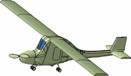
Fig. 2 Product drawing of general aviation aircraft project.

Table 1 Development costs and related parameters.27

Fig. 3 Main parameters affecting general aviation aircraft costs.

It can be concluded from Table 2 that the absolute percentage errors of these two benchmark samples are 4.0% and 3.7%, respectively, which means that both the two estimated development costs are accurate.Fig.5 shows the fitting results using the PLSR method and the prediction results for the benchmark samples. It is obvious that this method has good fitting and prediction behavior for the general aviation aircraft data.

4.2.2. BP method analysis

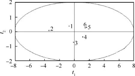
Fig. 4 Judgment ellipse of first six sample points.

The first six samples are analyzed by the BP neural network method. Eight cost influencing parameters and the predicted development cost are included in the input and output layers.Additionally, nine is selected as the number of hidden layer nodes. The epoch number, target error, and initial value of the learning rate are set as 1000,0.0001 and 0.05,respectively.Purelin and tansig transfer functions are employed for the output and hidden layers, respectively. Fig. 6 shows the interface of the BP method for training in MATLAB.

Table 2 Prediction results of PLSR method.

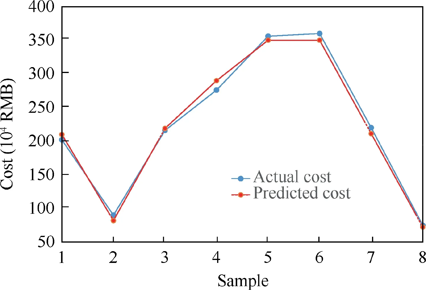
Fig. 5 Comparison between actual and predicted costs using PLSR method.

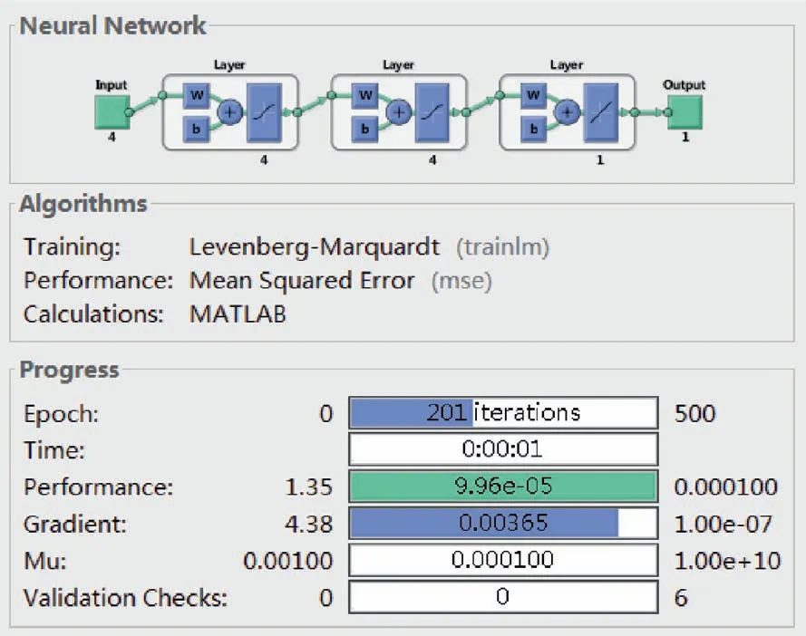
Fig. 6 Interface of BP method for training in MATLAB.

Table 3 Prediction results of BP method.

Then, the seventh and eighth samples are inputted into the learned network, and the predicted results and errors are included in Table 3.

Fig.7 shows the fitting results using the BP method and the prediction results for the benchmark samples.The results indicate that this method can be used to make a preliminary estimation; however, as indicated by the error rate, the average predicting error value and the error value of the eighth sample are 13.83% and 20.31%, respectively, implying poor prediction performance. This also confirms the conclusions drawn by Dongand Wang et al.the prediction performance of the BPN model is poor in cases of small sample size.

4.2.3. SR method analysis

The first six samples in Table 1 are fitted with the SR method using MATLAB 2015 software. Fig. 8 shows the interface of variable screening by the SR method in MATLAB software.

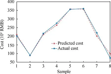
Fig.7 Comparison between actual and predicted costs using BP neural network method.

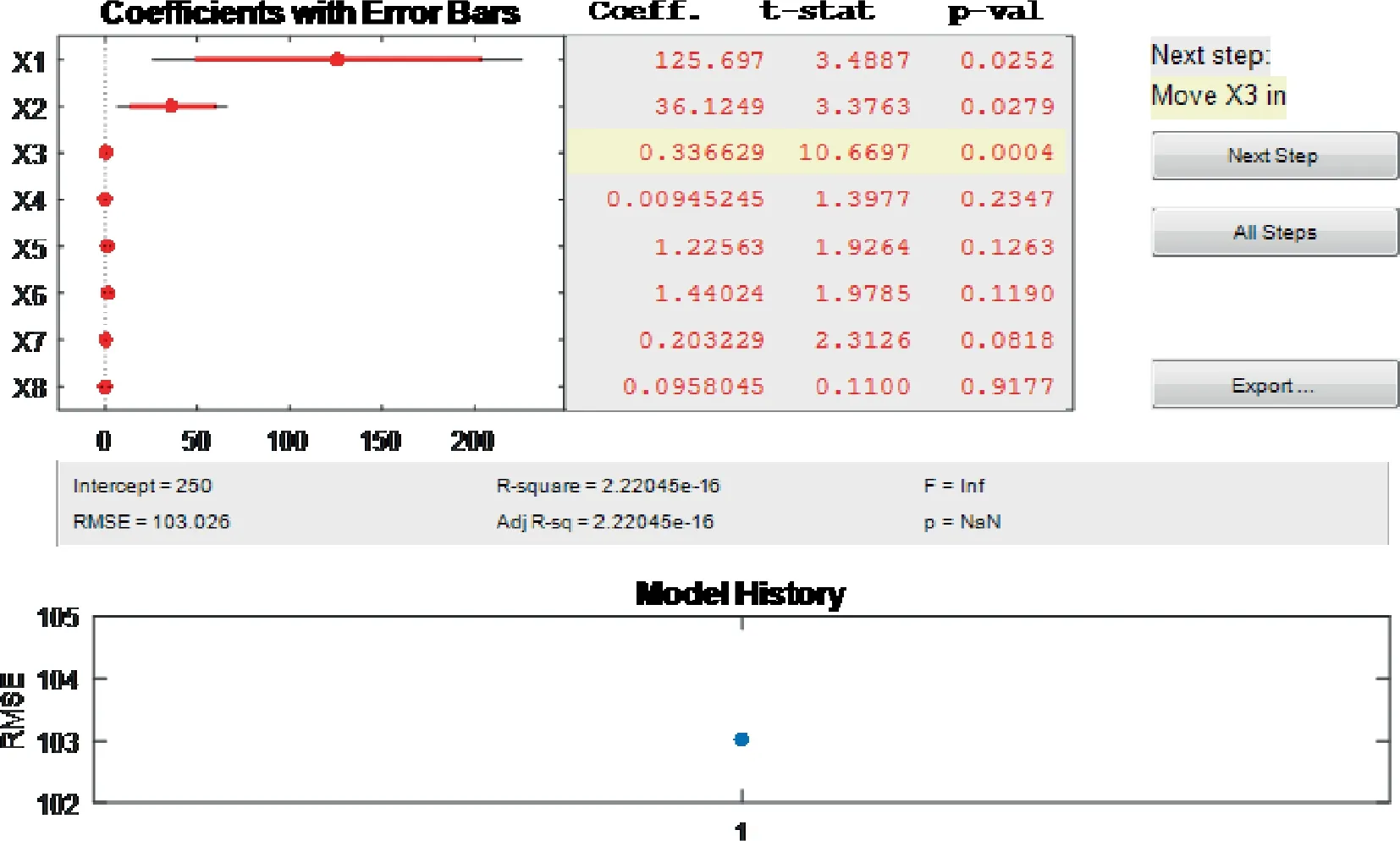
Fig. 8 Interface of variable screening (X1-X8 representing design parameters of general aviation aircraft) by SR method in MATLAB software.

Through the variable screening, only W, v, and Dare selected to build the regression model, and the SR regression equation is derived as The results predicted by the SR method are listed in Table 4.Fig.9 shows the comparison between the actual and predicted development costs by the SR method.The results indicate that the SR method, a single prediction method, exhibits a good prediction effect, with an average predicting error of 3.90%.Thus, it can be utilized for the initial estimation of development costs with relative accuracy.

4.3. Combined prediction method modeling The prediction results of the three single prediction methods for the benchmark samples are listed in Table 5.

Table 4 Prediction results of SR method.

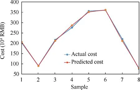
Fig. 9 Comparison between actual and predicted costs using stepwise regression method.

Table 5 Comparison of prediction errors of three single prediction methods.

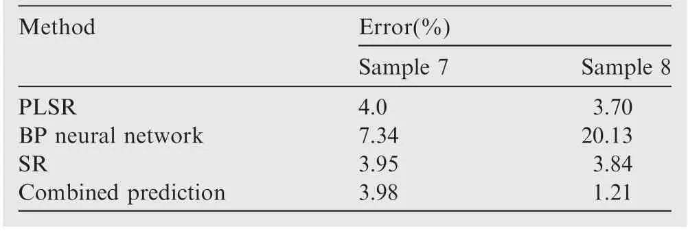
Table 6 Fitting results for benchmark samples.

where Y is the result of the combined prediction method, and y, y, yare those predicted by the PLSR model, BP model and SR model, respectively.

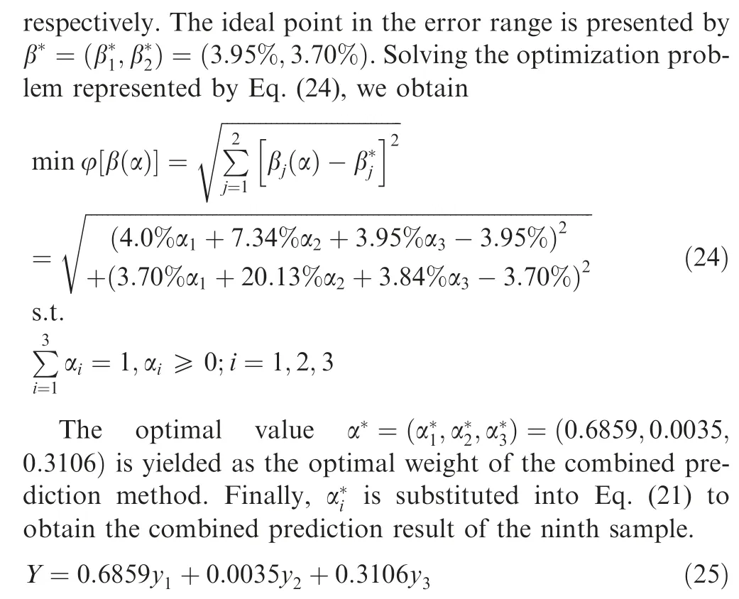
The optimal weight value indicates that the PLSR method has the largest weight in the combined prediction method,indicating that this method not only has the best prediction effect,but impacts the combined prediction result to the largest extent. The optimal weight value of the BP neural network method is only 0.0035, indicating little effect of this method on the combined prediction result.

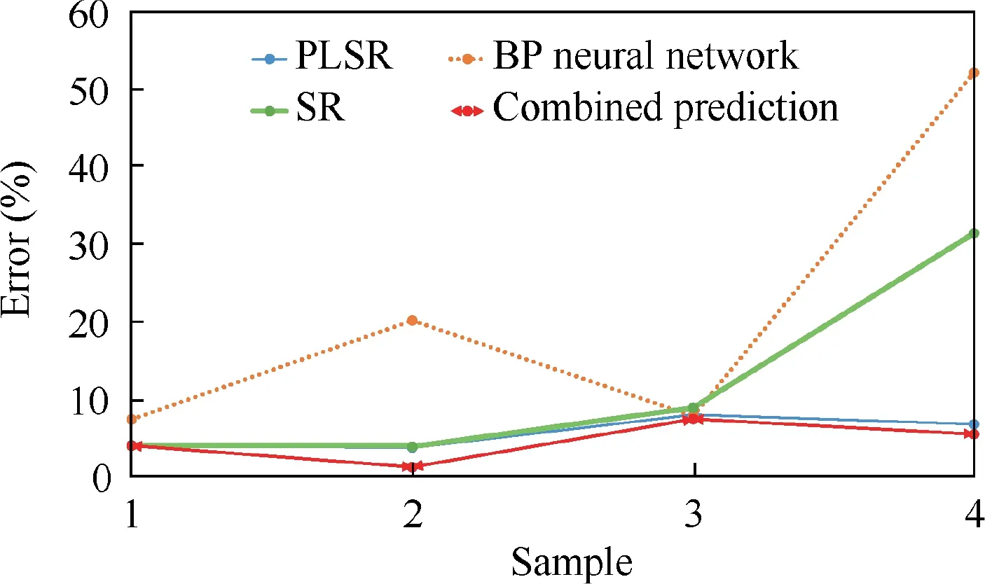
Fig. 10 Errors between single and combined prediction methods.

5. Simulation and results

The fitting results of the combined and single prediction methods on the benchmark samples are listed in Table 6,suggesting that the absolute percentage errors of the combined prediction method for benchmark samples 7 and 8 are 3.98%and 1.21%,respectively. In general, this fitting effect is better than that of all the three single prediction methods.

The ninth and tenth samples are predicted by the combined estimation method and the three single estimation methods.The prediction results are listed in Table 7, showing that the predicted development cost as per the combined prediction method is the closest to the actual cost compared to the values calculated by the single prediction methods, with the absolute percentage errors of 7.40% and 5.45%, respectively.

Fig. 10 shows the absolute percentage errors between the three single methods and the combined prediction method.As illustrated in Fig.10 and Tables 6 and 7,the combined prediction method has smaller fitting and predicting errors than the PLSR method,BP method,and SR method.Additionally,the results obtained by the PLSR method are closer to those of the combined prediction method, indicating that the PLSR method has the largest influence on the combined prediction results, which also corresponds to its weight factor of 0.6859.By contrast, the average fitting and predicting errors of the BP method are the maximum values of 13.83% and 29.98%,respectively, which largely reflects its unsuitability for small sample data.

In addition, data of military and civil aircraft are collected to verify the versatility of the combined prediction method and whether this method is always superior to single prediction methods despite the nature of the data.

Case 2. The data of military aircraft are listed as Table 8.Eight major independent parameters affecting the development cost are identified, namely, length of the fuselage (L),maximum take-off weight (W), height of the fuselage (H),take-off distance (D), maximum range (R), maximum level speed(v),empty weight(W),and maximum oil load(W).

Table 7 Predicted results.

Table 8 Data of military aircraft.

Table 9 Fitting and prediction results of military aircraft.

The first six groups of data are used to establish the three single prediction models, while the seventh and eighth groups of data are utilized as benchmark samples to determine the combined prediction model. The ninth group of data is used to test the model. The fitting and prediction results of the single and combined prediction methods on the benchmark and test samples are included in the table below.

It can be seen from Table 9 that the combined prediction method is better than the single prediction methods in terms of fitting and prediction performance. We also highlight the fact that the results of the SR method are close to those of the combined prediction method, indicating that the SR method has the largest influence on the results of the combined prediction method. To present the performance of the three single and combined prediction methods more directly,we plot the absolute percentage errors in Fig. 11.

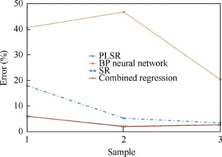
Fig.11 Errors between single and combined prediction methods for military aircraft data.

As shown in Fig. 11, for military aircraft data, the combined prediction method can still provide better prediction accuracy than each of the three single prediction methods.Although the prediction accuracy is only slightly higher than that of the stepwise regression method, aircraft designers would still be better served using the combined prediction method.

Case 3. To improve our assessment of comparability, data of civil aircraft are collected and analyzed (Table 10, Mis maximum thrust,Mis maximum ceiling,Mis maximum oil load).

The first six groups of data are utilized to build the abovementioned three single prediction models, while the seventh and eighth samples are used as benchmark samples to determine the combined prediction model.The ninth group of data is used to test the model. The absolute percentage errors of each single and combined prediction methods on the benchmark and test samples are seen in Table 11 and Fig. 12.

Table 10 Data of civil aircraft.

Table 11 Fitting and prediction results of civil aircraft.

Fig.12 Errors between single and combined prediction methods for civil aircraft data.

Comparison of Fig. 12 with Figs. 10 and 11 indicates that the prediction performance of the combined prediction method is better than all the single prediction methods introduced in this work with regard to both fitting and predicting performance. Moreover, the combined prediction method is not limited by aircraft types, which means that it can be used for the development cost prediction of general aviation aircraft,military aircraft,and civil aircraft.The combined prediction method presented in this study can effectively predict the cost of aircraft with reasonable accuracy even if the prediction accuracy may be only slightly higher than that of a single prediction method in some cases, because even this minor difference can contribute significantly to lowering the overall cost.

6. Conclusions

This study focuses on combining the PLSR,BP and SR methods to solve the problems encountered in cost estimation. The combined method has better estimation accuracy than the three single prediction methods, with less than 3% and 7%average fitting and prediction error values, respectively. We also find that the BP neural network method has a relatively large error, with more than 13% and 29% average fitting and prediction error values, respectively, suggesting that this method has poor prediction performance in this case and is not suitable for small sample data. A similar conclusion is reached when comparing military and civil aircraft development cost data.This research verifies the feasibility and usefulness of the combined prediction method in the development cost prediction domain as well as contributes to the literature by filling in the gaps of accurate development cost prediction for aircraft. The disadvantage of the combined prediction method is that it takes a part of benchmark samples to determine the optimal weight of each single prediction method,which may decrease the accuracy of each single prediction method. In future work, a real industrial general aviation aircraft product-development cost database could be considered to verify the effectiveness of the proposed combined method.Additionally, the optimal weight optimization method must be considered for further comparative study.

Declaration of Competing Interest

The authors declare that they have no known competing financial interests or personal relationships that could have appeared to influence the work reported in this paper.

Acknowledgement

s

This research has been supported by the National Postdoctoral Program for Innovative Talents, Postdoctoral Science Foundation of China(No.2017M610740). Also, the authors would like to acknowledge the supports from Hefei General Aviation Research Institute, Beihang University.