Axial response and material efficiency of tapered helical piles

Hamid Mortazavi Bak, Amir M. Halabian, Hamid Hashemolhosseini,Mohammadali Rowshanzamir

Department of Civil Engineering, Isfahan University of Technology, Isfahan, 84156-83111, Iran

Keywords: Tapered helical pile Axial response Bearing capacity Shaft resistance Initial tangent stiffness Relative material efficiency Taguchi method

ABSTRACT

1. Introduction

The response of axially loaded open-ended pipe piles as offshore or onshore deep foundations used in the construction industry has been widely investigated(e.g.Sakr and El Naggar,2003;Igoe et al.,2011; Yu and Yang, 2012; Fahmy and El Naggar, 2017a, b; Elsawy et al., 2019; Aghayarzadeh et al., 2020). Given the importance of material efficiency in the construction industry, different researchers tried to improve this parameter through an optimization process for geometrical design (e.g. Hataf and Shafaghat, 2015;Kolivand and Rahmannejad, 2018a; Tavasoli and Ghazavi, 2020).The tapered piles have been extensively investigated as a technique to increase the shaft resistance and bearing capacity of cylindrical deep foundations (e.g. Wei and El Naggar,1998; Sakr et al., 2004;Paik et al.,2011;Fahmy and El Naggar,2017b;Tavasoli and Ghazavi,2020).Wei and El Naggar(1998)experimentally displayed that the body resistance of tapered helical piles could be 40%more than the corresponding value of cylindrical piles. However, this value was reported up to 188% by Sakr and El Naggar (2003). Experimental studies conducted by Paik et al. (2011) and Kodikara and Moore(1993) also showed that the resistance force of tapered piles continuously increases by increasing the settlement.For piles with straight wall, the full skin resistance can be mobilized at the settlement of 2%of the pile diameter.The numerical analyses of Hataf and Shafaghat (2015) confirmed that the material efficiency of tapered helical piles is higher than that of cylindrical piles(i.e.up to 11%increase in the pile axial capacity with the optimum geometry).The decrease in circumference with depth is the main reason for the increase in the shaft resistance of tapered helical piles. Moreover, Tavasoli and Ghazavi (2020) showed that a tapered pile can provide a better durability performance and higher driving operation efficiency in comparison with straight-sided piles.

Besides tapered piles, helical piles constructed by welding helices to the open-ended pipe piles are another way to increase the material efficiency of open-ended piles. In 1836, the helical piles were first put into practice in the screw-pile lighthouse(Mohajerani et al.,2016).Helical piles were then widely utilized in the construction industry after invention of hydraulic helical pile drivers, since the installation process of helical piles needs both torque and crowd force simultaneously. The main advantages of helical piles are as follows:simple and quick installation,ability to carry loads sooner after installation, material-efficient and environment-friendly pile foundation (Mohajerani et al., 2016). The axial behaviors of these piles have also been investigated over the recent years(e.g.Mohajerani et al.,2016;Elsawy et al.,2019;Li and Deng, 2019).

By combining the concepts of helical and tapered piles, Fahmy(2015) first introduced the tapered helical pile, a new piling system. Previous studies confirm that geometrical properties of tapered helical piles (i.e. spacing and diameter of helices) can significantly affect the axial and lateral responses. However, few studies examined the effects of geometrical properties on the axial responses and failure mechanism of tapered helical pile separately(e.g. Fahmy, 2015; Fahmy and El Naggar, 2016, 2017b). In this context, a series of experimental and numerical analyses was carried out to examine the effects of different parameters on the axial response of tapered helical piles. By using the analysis of means(ANOM), the optimum geometry of a tapered pile is determined and the results of the analysis of variance (ANOVA) are used to calculate the degree of participation(DOP)of all factors that affect the performances of tapered helical piles,i.e.taper angle(θ),ratio of helix diameter to the average pile shaft diameter (D/dave), and spacing ratio(S/D).The capability of the Taguchi method to predict the ultimate bearing capacity and initial stiffness is also evaluated by comparing the experimental results with Taguchi method predictions. Finally, the pile with the optimized dimensions is compared with other model piles in terms of relative material efficiency factor.

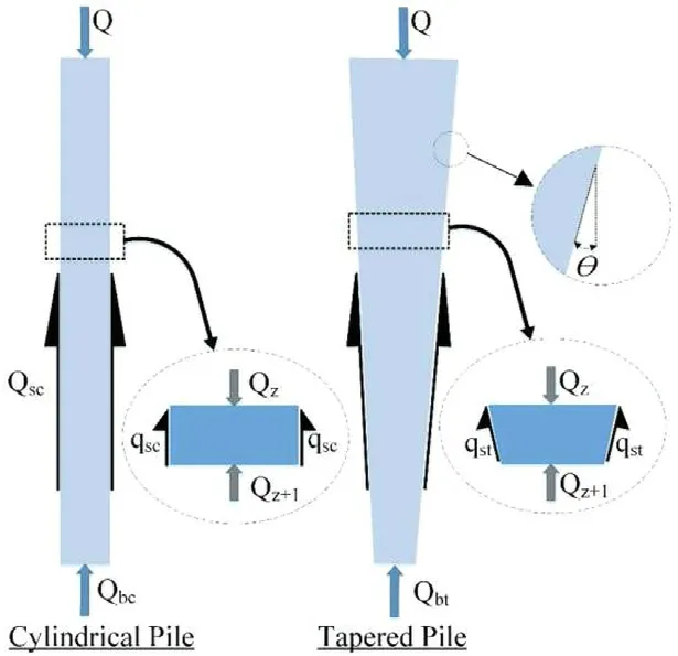
Fig.1. Geometry and stress distribution of cylindrical and tapered piles.

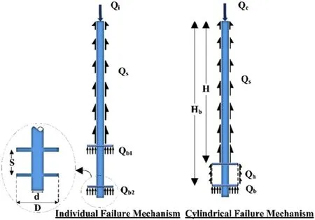
Fig. 2. Schematic diagrams of individual and cylindrical failure mechanisms.

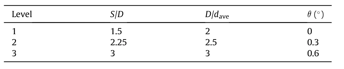
Table 1 Factors and their values at three levels.

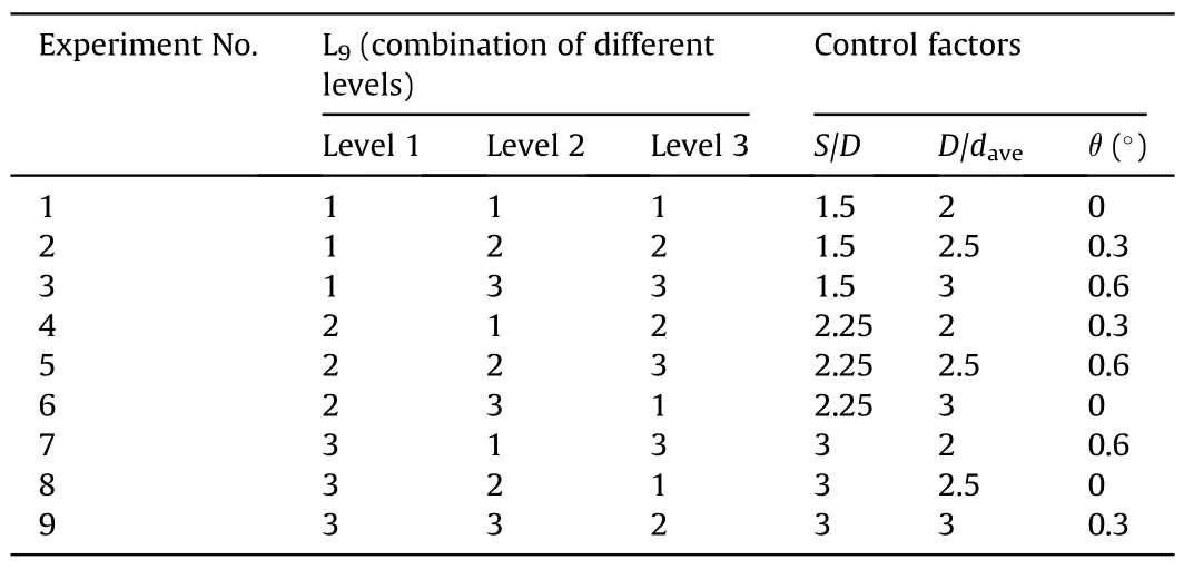
Table 2 L9 experimental design table.

2. Bearing capacities of tapered and helical piles

In order to gain a better view on the concept of combining the helical and tapered piles, the axial compressive responses of both tapered and helical piles are separately presented. Wei and El Naggar (1998) suggested the following equation to predict the skin friction along tapered piles:

where Ksis the coefficient of lateral earth pressure, σ′vis the effective vertical stress at the section level, δ is the soil-pile interface angle, and Ktsis the taper coefficient which can be calculated as follows (El Naggar and Sakr, 2000):

where θ is the pile taper angle; G is the sand shear modulus; Sris the pile settlement at the ultimate load level normalized by the pile diameter;and ζ=ln(rl/rm),in which rlis the pile radius at which the shear stress becomes negligible, and rmis the average pile radius.

In another study,Paik et al.(2013)defined the taper effect factor TFs,instead of Kts,to calculate the skin friction of tapered pile using the following relation:

where Dris the relative density of soil. Given Eqs. (1)-(3), θ, δ, σvand Drare the main parameters that influence the skin friction of tapered piles. Paik et al. (2013) did not take the effect of σvinto account while its effect has been proven in former studies (e.g.Kodikara and Moore,1993; El Naggar and Wei,1999). Fig.1 shows the friction resistance along the surface of tapered and cylindrical piles.

For helical piles, the ratio of helix spacing to helix diameter (S/D), called spacing ratio, is an important factor to determine the mechanism of failure in terms of the axial response of helical piles.Individual and cylindrical failure mechanisms are the two possible failure mechanisms of helical piles,as shown in Fig.2.As a general rule,it can be stated that the more the S/D value raises,the higher the probability of individual failure mechanism increases.However,different researchers have proposed various boundary values for S/D to determine the type of failure mode. For example, Rao et al.(1991) observed that if S/D becomes smaller than 1.5, the cylindrical failure mechanism will occur, while S/D equal to 3 was suggested as the boundary value by some of the other researchers(e.g.Aydin et al.,2011;Tsuha et al.,2013).On the other hand,Lutenegger(2009) and Nasr (2009) proposed that for S/D values higher than 2.25 and 2, respectively, the cylindrical failure mechanism would change into the individual mechanism. In the individual failure mechanism, each helix is loaded individually, while in the cylindrical failure mechanism, only the bottom helix is loaded (see Fig. 2). It is noteworthy that the type of failure mechanism is affected by other parameters such as soil type and density.

Fig. 3. Schematic of model pile.

The cylindrical shear method was first used to calculate the bearing capacity of helical piles by Mitsch and Clemence (1985).The cylindrical shear method assumes that the pile compressive bearing capacity is equal to the sum of the surface shear resistance of the soil cylinder located between the helices and the bearing capacity of the bottom helix (Fig. 2). Accordingly, the bearing capacity of a helical pile installed in the sand can be calculated using the following equation:

where H is the embedment depth of the first helix, D is the diameter of pile helix,d is the diameter of pile shaft,Heffis the effective length of pile above the helix(Heff=H-D),γ′is the effective unit weight of soil,Nqis the bearing capacity factor for cohesionless soils(Meyerhof,1976),Psis the pile shaft perimeter,AHis the area of the lower helix, and φ is the soil friction angle (see Fig. 2).

The individual failure mechanism was first introduced by Trofimenkov and Mariupolskii (1965). As shown in Fig. 2, the compressive bearing capacity of the helical pile is equal to the summation of the shaft resistance and bearing resistance of helices individually (Adams and Klym, 1972). Accordingly, the following equation can be defined,which deals with the compressive bearing capacity based on the specific failure mechanism:

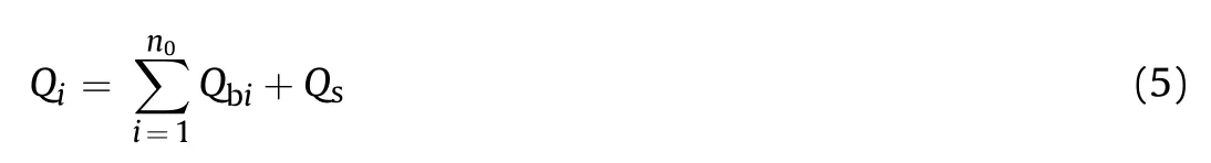
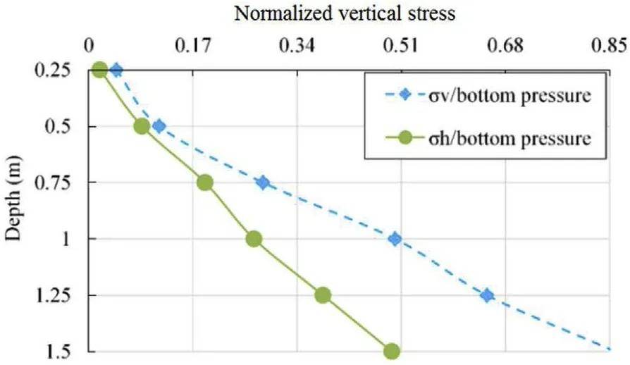
Fig. 4. Normalized stress variation along the centerline of FCV.

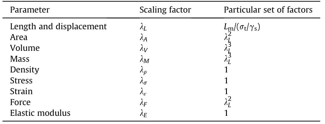
Table 3 Scaling factor requirement for the pile-soil system (Sedran et al., 2001).

where n0refers to the number of helices, and Qbiand Qsare the bearing resistance of the ith helix and the shaft resistance,respectively.

3. Experimental design

According to Elsherbiny and El Naggar (2013), the most commonly used helical piles are the piles with two helices rather than the piles with three helices or even one helix. On the other hand, individual and cylindrical failure mechanisms are the only analytical failure mechanisms recognized in the literature. As discussed previously, the spacing ratio S/D is the main factor controlling the failure mode,and different values varying between 1.5 and 3 are proposed with which the cylindrical failure mechanism changes from cylindrical into individual mechanism.

Another parameter that affects the performance of tapered helical piles could be the pile taper angle.Hataf and Shafaghat(2015)showed that the optimized taper angle of a single pile with which the maximum bearing capacity can be reached is a function of the soil internal friction angle.It was suggested that the optimal taper angles for the soil with internal friction angles equal to 33°,38°and 43°are 0.4°, 0.8°and 1.2°, respectively. They also concluded that the bearing capacity of tapered piles with optimal taper angle installed in sands with φ = 33°, 38°and 43°increases by 2.6%, 7%and 11%, respectively, in comparison with that of cylindrical piles with the same volume. Therefore, in the current study, the taper angle (θ), the ratio of helix diameter to the average pile’s shaft diameter (D/dave) and the spacing ratio (S/D) are selected as the main parameters (Table 1).

The Taguchi design of experiments(TDOE)method was used to design experiments. The TDOE method was introduced first by Taguchi (1986) who derived a family of fractional factorial experiment matrices that have been employed in different fields including geotechnical engineering (Kolivand and Rahmannejad,2018a, b; Lafifi et al., 2019). This method can be used to minimize the experimental costs(Chou et al.,2009).According to the number of factors and their levels, L9orthogonal array was used in this study(Table 2). Orthogonal arrays are used to lay out experiments in TDOE method.The schematic of the model pile is plotted in Fig.3.All model piles are designed with equal volume. It is noteworthy that the average diameter of all the model piles is 4.2 cm and all of the model piles are open-ended.

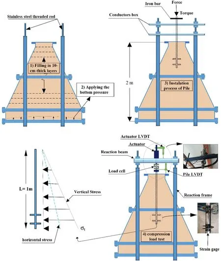
Fig. 5. Schematic diagram of the FCV testing procedure.

4. Experimental setup and procedures

Different apparatuses are used to examine the compressive responses of axially loaded piles, such as rigid chamber (Ullah et al.,2018), calibration chamber (Lee et al., 2012), geotechnical centrifuge(El Naggar and Sakr,2000)and frustum confining vessel(FCV)(Horvath, 1995; Horvath and Stolle, 1996; Sedran et al., 2001;Karimi and Eslami, 2018; Moshfeghi and Eslami, 2019). The experimental setup contains a FCV apparatus built in Isfahan University of Technology,model piles,a hydraulic jack/actuator,a load cell, two linear vertical displacement transducers (LVDTs) and a data acquisition (DAQ) system. The FCV used in this study has top and bottom radii equal to 40 cm and 180 cm,respectively.Its total height is 196 cm (Mortazavi Bak et al., 2020).

After pouring the soil into the FCV in 10-cm thick layers using the air-pluviation method with the relative density of 25%,the base pressure was applied to the bottom of the soil sample. The base pressure causes an almost linear stress distribution varying between zero at the surface and bottom pressure at the bottom of the soil along the centerline of the FCV.The variation of the normalized vertical and horizontal stresses along the centerline of the FCV was recorded using the pressure cells located at different levels along the centerline(Fig.4).The uniformity of the samples is also verified by measuring local densities in cylindrical molds at different locations of the FCV.Given the stress at the bottom of the pile,the unit weight of the soil sample and the length of the reduced-scale pile,the geometric scale ratio (λL) is given by

where Lmis the length of the model pile,σtis the vertical stress at the pile bottom, and γsis the unit weight of soil. Lm, σtand γsare equal to 1 m, 60 kPa, and 15 kN/m3herein, respectively; hence,λLequals 0.25 for all of the pile models.Sedran et al.(2001)obtained appropriate scaling factors for the FCV testing technique,as given in Table 3.

As shown in Fig. 5, the head of the model piles was instrumented by a 20 kN S-typed load cell and two LVDTs with a range capacity of 50 mm and 0.05% linearity to probe the load and displacement in conjunction with strain gages(i.e.TML strain gages of type FLA-6-11) installed on the pile surface to evaluate the load variation along the model piles.After the strain gages are installed and the surface is coated,they are calibrated by applying load to the head of piles. Ultimately, the pile compression load test is performed based on ASTM D1143/D1143M-07(2013)e1 (2013). As shown in Fig.6, all of the model piles are loaded at least up to the displacement ratio of 0.15 and the pile head displacements of all the model piles are more than 15%of helices diameter at the end of the pile load tests subsequently.

Soil properties are given in Table 4. It is noted that the soil grading is not scaled since the behavior of sand is highly dependent on its grain size and shape.Previous studies showed that if the ratio of the average pile shaft diameter to the mean grain size of sand(dave/D50) is more than a limiting value varying between 30 and 100, the grain size effect would be negligible (e.g. Mortazavi Bak et al., 2020). The average pile shaft diameter of all the model piles is 42.2 mm, which means that dave/D50is equal to 200.

Fig. 6. Load-displacement curves of reduced-scale piles.

Table 4 Summary of sand properties.

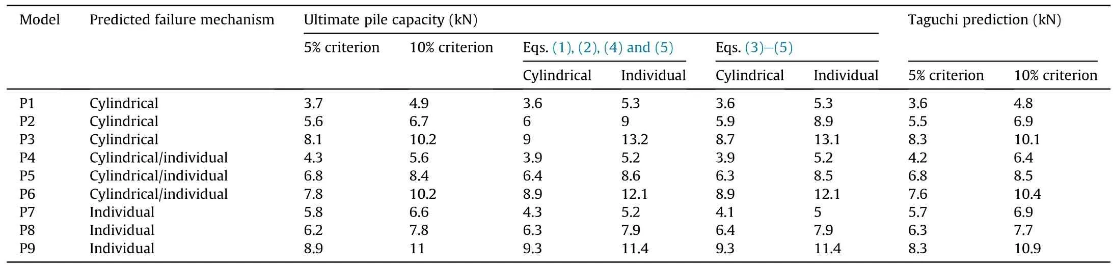
Table 5 Ultimate pile capacity obtained from axial compression load tests and Taguchi predictions.

5. Results

In this section,the load-displacement curves obtained from the axial compression load tests are discussed. The pile head displacement is presented in terms of displacement ratio,which is defined as the ratio of the pile head displacement to the helix diameter around the pile(Δr).The results recorded by strain gages are used in conjunction with the load-displacement curves to evaluate the frictional behavior of pile along its shaft. Then, the material efficiency of different pile shapes is compared, and the optimum geometry is proposed.Finally,the initial tangent stiffness(K0)of model piles is evaluated,and the effect of geometry on this factor is discussed.

5.1. Load-displacement curves

As observed in Fig.6,the load at the head of the tapered helical piles increases continuously while this trend is not seen in the helical piles. This is mainly caused by the skin friction of tapered piles which increases continuously with increasing settlement.This phenomenon could be related to the increase of normal stress on the surface of tapered piles by applying displacement to their heads,while the normal stress is almost constant in the cylindrical piles during the settlement. Hence, through comparing tapered helical piles and helical piles in terms of plunging failure, tapered helical piles show better behavior. The findings of this study regarding the behavior of tapered helical piles are consistent with those of Sakr et al. (2004).

Pile head load at displacement equal to 10%of the pile diameter is defined as the ultimate bearing capacity of the pile by Terzaghi(1942). On the other hand, O’Neil and Reese (1988) defined it as the load at 5%of pile diameter.Given that the pile head settlement is limited to the settlement tolerance which is less than 25 mm(Sakr et al.,2004)and the maximum prototype pile helix diameter is 501 mm,the results are compared in both 10%(Nasr,2009;Sakr,2009, 2011) and 5% (Sakr, 2009, 2011) of pile head settlement approaches. Table 5 summarizes the axial compression load test results (i.e. mean values). The predictions of the Taguchi method based on the compressive bearing capacity are also presented in Table 5. As seen in Fig. 7, the results of ANOM show that the optimum level of all three of S/D, D/daveand θ is the third one,considering that higher ultimate bearing capacities are desired.

Fig.8 shows the predicted values of compressive bearing capacity of reduced-scale tapered piles versus the test results for both 5%and 10% pile head settlement criteria. The coefficients of determination(R2) of the relationship between Taguchi predictions and experimental results according to 5%and 10%criteria are 0.985 and 0.997,and their average relative errors are 2.54% and 1.54%, respectively.Hence,forthe modelpiles,theabilityof the Taguchi method topredict the compressive bearing capacity of tapered helical piles in response to different combinations of factor/levels is confirmed.

To understand the effect of each factor,by changing the level of each factor while the other factors are kept constant at the first level,the variation of ultimate bearing capacity is plotted in Fig.9.As could be seen, by changing the level of D/dave, the bearing capacity was increased more considerably in comparison with other parameter variations.

Fig. 7. Plots of main effects: (a) 5% and (b) 10% criteria.

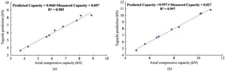
Fig. 8. Taguchi predictions versus experimental results using Taguchi analysis: (a) 5% and (b) 10% criteria.

Fig. 9. Variation of bearing capacity at different levels for each factor while other factors are kept at the first level: (a) 5% and (b) 10% criteria.

5.2. Shaft skin friction

The shaft resistance is probed using strain gages located at the distances equal to H/2 (SG1) and H (SG2) from the pile head. The predicted values of Ktsare plotted in Fig.10 based on Eqs. (2) and(3). It is obvious that the values of Ktsare highly dependent on the stress levels. These observations are in compliance with the results shown in Fig. 11 and relevant previous studies (e.g.Nordlund,1963; Ladanyi and Guichaoua,1985; Wei and El Naggar,1998;El Naggar and Sakr,2000).The average values of Ktsfor upper and lower halves of the second pile are equal to 1.94 and 1.35,respectively,while they are 2.62 and 1.65,respectively,for the third model pile.Although Nordlund(1963)and Ladanyi and Guichaoua(1985)attributed the increase of the tapered pile skin friction to the increase of confining stress adjacent to the pile and compaction of the soil close to the pile Surface, the frictional behavior is highly dependent on the installation techniques,i.e.head driving and toe driving,as investigated by Sakr et al.(2004).The primary deficiency in the literature is that the effect of disturbance caused by the helices and passed through the soil during the installation process of tapered helical piles is not yet examined. According to the results,Kstis nearly close to the values calculated by the equation delivered by Wei and El Naggar(1998)at low-stress levels.However,it keeps close to the relationship proposed by Paik et al. (2011) at highstress levels.

Fig.10. Variation of Kst according to Wei and El Naggar (1998) and Paik et al. (2013).

Table 6 Initial stiffness obtained from axial compression load tests and Taguchi prediction.

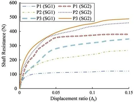
Fig.11. Shaft resistance versus pile head displacement.

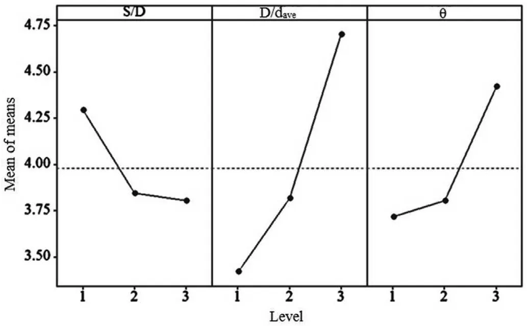
Fig.12. Plots of main effects for different parameters at different levels.

5.3. Initial tangent stiffness

Fig.11 shows that by increasing the taper angle,the skin friction absorbs more forces at low strain levels compared to straight wall piles, which means that it could increase the pile initial stiffness.The initial stiffness is an important parameter that plays a key role in the pile response at low excitation levels. In view of this, the effect of each parameter on the initial stiffness is examined and presented in Table 6. Fig. 12 shows the optimum levels of each parameter. The optimum level is the first one for spacing ratio,while the third level is the optimum level for D/daveand θ,when the initial stiffness is considered.

Given Table 6,Fig.13 plots the predicted values of reduced-scale tapered piles’ initial stiffness versus the test results. The coefficient of determination (R2) of the relationship between the Taguchi predictions and experimental results is 0.979,with average relative error of 2.33%. Hence, for the test model piles, the ability of the Taguchi method for predicting the initial stiffness of tapered helical pile in response to different combinations of factor/levels is confirmed.

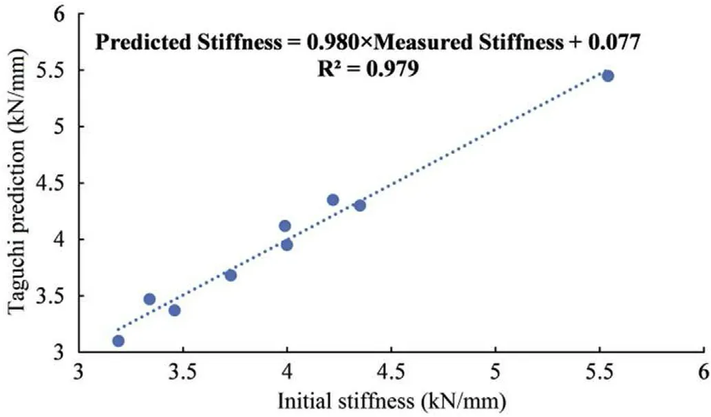
Fig.13. Taguchi predictions versus experimental results.

6. Signal-to-noise and variance analyses

Signal-to-noise analysis has been used widely to analyze the experimental results of the Taguchi method. It is significant to determine the optimum geometry in which the bearing capacity and initial stiffness approach their maximum values, thus the signal-to-noise ratio(S/N)with higher better(HB)criteria has been applied (Taguchi, 1986; Kolivand and Rahmannejad, 2018a; Lafifi et al., 2019). Accordingly, S/N value for the HB type is given by the following equation:

Table 7 Summary of signal-to-noise analysis results for different parameters.

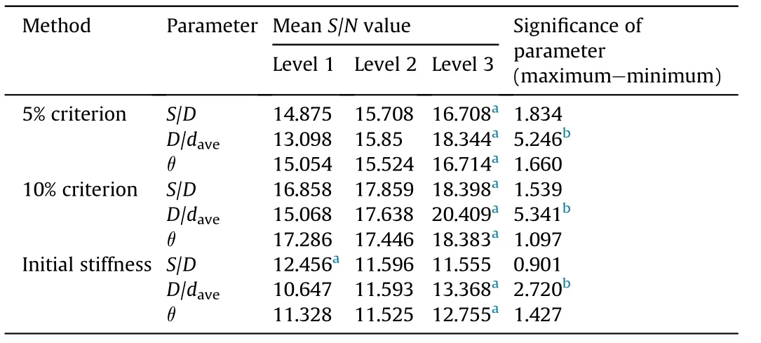
Table 8 Summary of ANOM results.

Table 9 Summary of ANOVA results.

Fig.14. S/N values at different levels: (a) 5% criterion, (b) 10% criterion, and (c) initial stiffness.

where r is the number of repetitions for each deigned experiment,and Yiis the result of the ith repetition.The results of the signal-tonoise analysis for 5%criterion,10%criterion and initial stiffness are presented in Table 7.

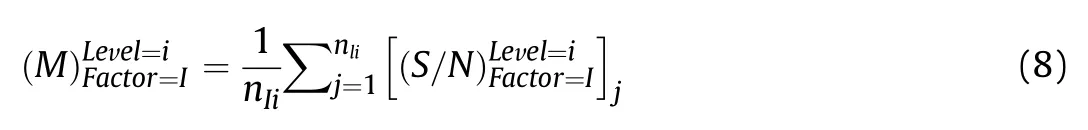
After obtaining the S/N values for different states,ANOM is used to determine the optimal condition for each factor. In this regard,the mean S/N value of each factor is determined at different levels using the following equation:

where nIiis the number of appearances of factor I in level i,and L is the number of levels of each factor. Using the signal-to-noise and ANOM analyses,the optimal level of each factor could be obtained.Table 8 and Fig. 14 show the results of the ANOM analysis. The optimum level of all the factors is the third one for bearing capacity,while this level is the first one for spacing ratio (Fig.14c) and the third one for others when the initial stiffness is considered. From Table 8, it is evident that D/daveis the most significant parameter.

Fig.15. Degree of participation of different factors.

Fig.16. Schematic of finite element mesh for optimum model.

To obtain the effect of each parameter on the results,ANOVA is used. The degree of participation (DOP) of each factor is the main output of the ANOVA analysis given by the following equations(Sadeghi et al., 2012):

where n is the number of experiments, DOFFis the degree of freedom of each factor,the average value of the test results of a specific factor in the kth level,and VEris the variance of error which could be calculated using the following equation:

where m is the number of model piles, and SSTis the total sum of squares given by the following equation:

Using aforementioned equations,ANOVA can be performed,and its results are presented in Table 9.As could be seen,D/davehas the highest DOP against other factors.The DOP of θ(ρF)is 2.59%for 10%criterion, and it is equal to 5.92% and 19.51% for 5% criterion and initial stiffness, respectively. The reason could be related to the factor that the interface resistance reaches its maximum values at lower displacements in comparison with bearing capacity of helices.Fig.15 shows the variation of the DOP of each factor according to different parameters.

Table 10 Properties of materials in finite element analysis.

7. Numerical analysis

To further examine the axial response of tapered helical piles,axisymmetric finite element models were developed using the finite element software ABAQUS. First, the capability of the axisymmetrical model to predict the axial response of tapered helical piles was examined using the experimental results of model piles Nos.3(configuration A)and 9(configuration B),and then the pile with optimum geometry(configuration C)(i.e.S/D,D/daveand θ were chosen as 3, 3 and 0.6, respectively) was modeled. Next, the numerical results are compared with the predicted values based on the Taguchi method and experiments.

7.1. Axisymmetrical model

Because of the symmetry of the material,geometry,and load of the experimental setup,axisymmetrical modeling was used as the most cost-effective numerical approach.Fig.16 shows the optimum model geometry of tapered helical pile installed in the FCV apparatus. The soil medium, FCV apparatus, and model piles were simulated using 3-node linear axisymmetric triangle elements(CAX3) having two active translational degrees of freedom. The boundary conditions at the first step of the simulation were as follows:rollers along the centerline of FCV and soil sample,stressfree boundaries at the top of the soil,interface elements at the side faces of the FCV, and fully fixed nodes at the bottom of the FVC.Since the deformation of the soil is greater in the zones close to the helices than that in the zones far from the helices, the mesh refinement has been applied in these zones.The soil medium in the simulated pile configurations A,B and C consisted of 7432,6473 and 5998 elements, respectively, with element dimensions varying between 0.1 cm and 12 cm.The model piles also consisted of 1340,1156 and 1256 elements for configurations A,B and C,respectively.The soil was modeled as an isotropic elastic-perfectly plastic Mohr-Coulomb material model, and the model piles and the FCV apparatus were simulated as a non-porous linear elastic material. The properties of the materials used in the finite element analyses are summarized in Table 10.

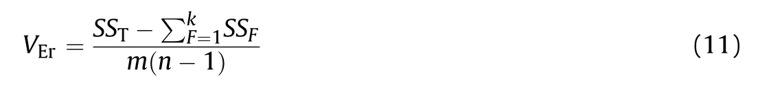
To model the soil-structure interfaces, the full contact algorithm which allows separation and sliding during the analysis in conjunction with a linear elastic-perfectly plastic Mohr-Coulomb frictional model was used in this study. To this end, a series of direct shear tests based on ASTM 3080-03(2003)and ASTM D5321/D5321M-13 (2013) was conducted to investigate the soil shear strength and the friction coefficient between the sand at low relative density (e.g. Dr= 25%) and steel. According to the experimental results,the friction coefficients(tanδ)of 0.32 and 0.46 were calculated for soil-pile and soil-FCV interfaces(i.e.the surface of the FCV was roughened), respectively. Fig.17 shows the schematic diagram of modified large shear test used in this study.

The self-weight of the materials was applied to the model in the first step. Then, the base pressure equal to 120 kPa was applied to the bottom of the soil elements defined by a ramp function with time span of 20 min.Subsequently,the model piles were modeled by applying the stresses of the soil sample elements derived in the previous steps to the model as predefined field stresses. Finally,using the reference point pinned rigidly to the pile head/cap, the pile head was subjected to the downward displacement at a constant rate.

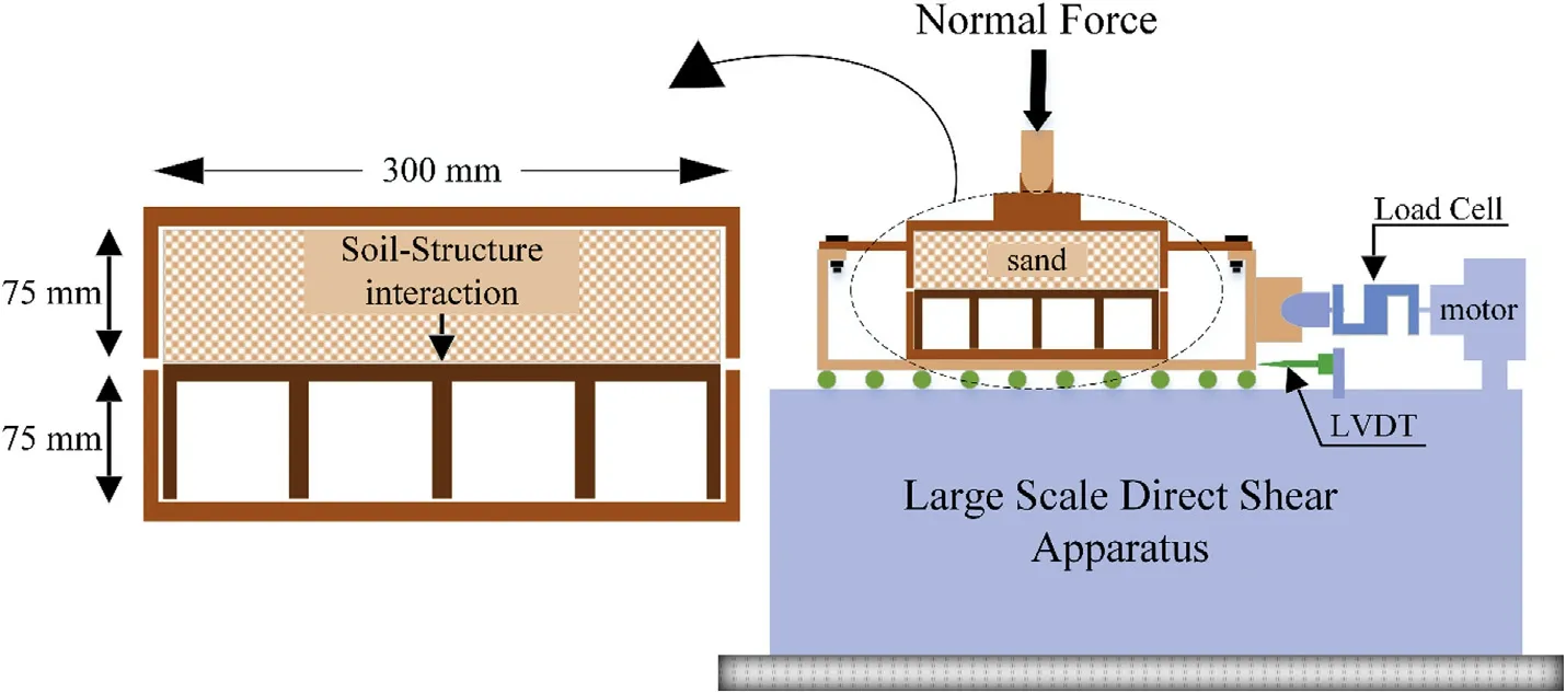
Fig.17. Schematic diagram of modified large direct shear test.

Fig.18. The load-displacement curves.

7.2. Numerical results

Fig.18 shows the load-displacement curves of model piles Nos.3 and 9 and the optimum model pile. In the current study, the installation effects are not considered in this numerical analysis.When it comes to installation effects, the compaction of the soil beneath the helices and the disturbance of the soil adjacent to the shaft (i.e. due to the shearing caused by the passage of helix through the soil) are the most important phenomena observed by Bagheri and El Naggar(2015)and Tsuha et al.(2012).Fahmy and El Naggar(2017a)stated that the effects of the disturbance of the soil adjacent to the shaft could be faded owing to the re-compaction of the disturbed soil. Therefore, after examining the numerical model’s capability to predict the axial behavior of piles and comparing the numerical and experimental results of all model piles, the installation effect factor (IEF) can be defined as follows:

where Qexpand Qnumare the ultimate bearing capacities based on experimental and numerical results, respectively; Comparison of numerical and experimental results reveals that IEF is equal to 1.06,meaning that the installation process could cause an increase in soil strength parameters. Therefore, this value is highly dependent on the procedure of installation. In light of these facts, the ultimate bearing capacities of the optimum model pile based on Taguchi prediction, experimental results, numerical analysis, and modified numerical prediction are obtained as 11.43 kN,11.72 kN,11.16 kN,and 11.83 kN, respectively. Fig. 19 shows the magnitude of displacement of the soil located between the helices in model pile No.3(i.e.S/D=1.5)and the optimum pile(i.e.S/D=3)at the pile head displacement equal to 10% of the helix. The difference between the individual and cylindrical failure mechanisms could be clearly observed.

8. Relative material efficiency factor

Considering the results of the axial response of the optimum pile, the relative material efficiency factor (RME) could be defined as follows:

Fig.19. Displacement contours (10% criterion): (a) cylindrical and (b) individual failures (unit: m).

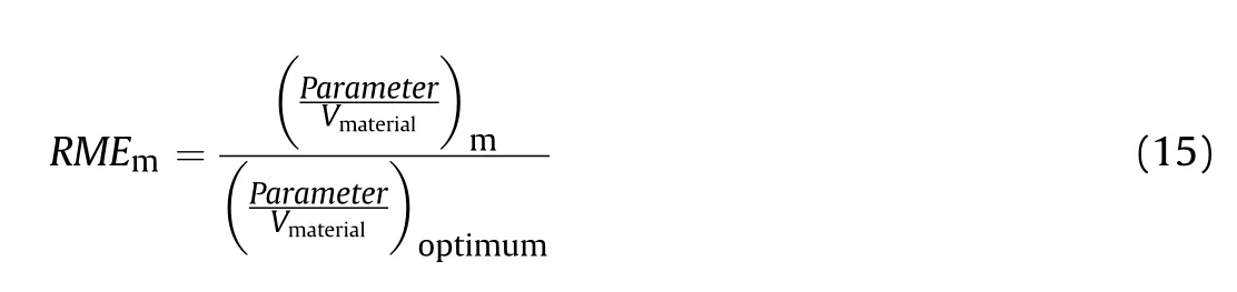
Fig. 20. Variation of RME for different model piles.

where parameter is the ultimate bearing capacity based on 5% or 10% criterion or initial stiffness, and Vmaterialis the volume of the material consumed in the pile. As observed, all of the piles are compared with the optimum one using the experimental results.Fig.20 shows the REM for different tapered helical pile geometries.Comparing RME1with RMEoptreveals the importance of geometry optimization.The relative material efficiency of the optimum pile is 2.5,2.38 and 1.67 times that of the first model pile.This means that the pile with the same volume of material but constructed in the optimum geometry could have higher bearing capacity and initial stiffness.

9. Conclusions

The axial compressive responses of tapered helical piles installed in loose sand were examined in the present paper. The ultimate bearing capacity, skin resistance, initial stiffness, and relative material efficiency factor are the main response parameters investigated. The following conclusions are made:

(1) The taper angle could increase the ultimate bearing capacity and initial stiffness of the pile simultaneously. In terms of bearing capacity, the DOP values according to 5% and 10%criteria are 6%and 3%,respectively.Considering the results of the initial stiffness,the taper angle’s DOP increases to 19.51%.Additionally,the effect of the taper angle is significant at low stress levels and decreases by increasing the stress levels; it could affect the initial stiffness of the tapered helical pile significantly. The results derived from load-displacement curves and strain gages also show that the skin resistance and the pile axial resistance are continuously increased as the tapered helical pile head moves downwards.

(2) The effect of spacing ratio(S/D)is proven and the DOP values are calculated as 7.9%,5.8%and 9%based on 5%criterion,10%criterion, and initial stiffness, respectively. According to the experimental and numerical results, S/D value equal to 3 is the optimum boundary value for determining the failure mechanism.

(3) The diameter of the helix is the main factor that could increase the bearing capacity of the tapered helical piles.However,limitations of pile structural failure should also be taken into consideration. The DOP values of D/daveare calculated as 83.9%, 90.2%, and 60.5% according to 5% criterion,10% criterion, and initial stiffness, respectively.

Nevertheless, the axial responses of tapered helical piles need further study in order to determine the relationship between wall inclination angle of the pile and the failure mechanism,installation effect, group pile effect, skin resistance factor, dynamic response,and others.

Declaration of competing interest

The authors declare that they have no known competing financial interests or personal relationships that could have appeared to influence the work reported in this paper.