Real-time recommendation based on comprehensive popularity of items

Yang-xin QIN，Biao CAI，Xin-ping ZHU

（College of Information Science＆Technology，Chengdu University of Technology，Chengdu 610059，China）

Abstract：In an age of explosive information growth，information has the attributes of timeliness，sharability，and relativity of value.Personalized recommendations can help resolve the difficulty in making choices for users who are confronted with information overload.The information aging problem is to be expected during the development of information networks，and incorporating the time factor into recommendation algorithms is becoming a trend.Most studies on recommendation algorithms considering the time factor have either focused on changes in users’ interests or the current popularity of items.However，the time-varying comprehensive popularity of items（Com-PI）has attracted little attention.In this study，a real-time recommendation algorithm based on ComPI was proposed.The main contributions of the present study were as follows：（1）the development stage of item in product life cycle was considered in the recommendation；（2）the time factor was incorporated into the recommendation algorithm，and an exponential time-weight decay model was built for the quantification of time weights；（3）the total probability model was combined with the time-weight decay model to establish the ComPI-based recommendation algorithm，which effectively solved the problem of“marketing myopia”in current algorithms；（4）the algorithm was tested on real data sets.The results showed that our real-time recommendation algorithm had better accuracy，diversity，and novelty；（5）we also researched the growth characteristics of data and its impact on data partitioning and algorithm performance evaluation，and proposed that we should pay more attention to the data with exponential growth when studying recommendation algorithms.In brief，this algorithm can effectively improve the user experience by using the time factor in recommendation systems.In addition，the ComPI model can also help to study the evolution process of network topology，and can be applied to network related fields.

Key words：Recommendation system，Real-time recommendation，Time-weight model，Comprehensive popularity

1 Introduction

Recommendation algorithms have become one of the most effective solutions for overcoming information overload［1］.They can help users glean the necessary information from massive amounts of information quickly and effectively［2］，and they have already become an integral component of e-business.For example，Amazon，Netflix，YouTube，and many other websites use recommendation systems to enhance user experience and satisfaction，ultimately increasing profits［3］.Collaborative filtering is one of the most extensively used and most effective recommendation algorithm［4-5］.Collaborative filtering is further divided into item-based collaborative filtering（ICF）［6］and user-based collaborative filtering（UCF）［4］.ICF is mainly used to recommend items similar to those al-ready bought by the users，and UCF，which focuses on users，is used to recommend items bought by users similar to the target users.

By introducing the principles of physical dynamics，Zhang et al.proposed the probabilistic spreading（ProbS）algorithm［7］and the heat conduction（HC）algorithm［8］.The former simulates the mass transfer process in physical dynamics by assuming the conservation of the total amount of resources，whereas the latter is based on an analogy with the constant transfer of heat between users and items in a bipartite graph.Since the total amount of resources keeps increasing，the probability of unpopular items being recommended increases.A combination of these two algorithms［9］effectively improves the diversity and accuracy of the recommended items.There is also the CosRA algorithm［10］，which integrates cosine similarity and the resource allocation index（RA）.In recent years，a recommendation algorithm based on the triangle area calculation mode［11-12］has been established，and this algorithm can dramatically improve the diversity of the items recommended.In addition，there are content-based recommendation algorithms［13-15］and hybrid recommendation algorithms［16-17］.

The conventional recommendation algorithm is mostly a process of bipartite-based simple resource allocation；however，in recent years，an increasing number of influencing factors have been considered.Zimdars et al.first incorporated time information into the recommendation algorithm when they performed a mapping of a recommendation problem into the problem of time series prediction［18］.Similarly，Wu et al.found that on Digg.com，a popular news platform，the freshness of nearly half of the news receded or the news became outdated or unpopular within a short period of time［19］.Under the classical collaborative filtering framework，many algorithms have incorporated the influence of time to enhance algorithm performance.Generally speaking，a user’s interest in a single theme decays over time.Ding and Li［20］reallocated the resource index by decreasing the weight of the outdated items，which was，in turn，represented by decay functions.Other algorithms transform collaborative filtering into a time-dependent iterative prediction problem，and a method with automatic allocation and update of the size of each user neighborhood has been proposed［21］.Additionally，simple time-biased KNN-based recommendations［22］showed that the use of information near the date of recommendation alone could help improve the recommendation performance and reduce information overload.

In addition to the time-varying popularity of items，user interests，hobbies，and tastes also vary with time.In this case，the ranking of the items in the recommendation list should also be adjusted over time［23-24］.Lathia et al.studied the time-varying diversity of recommendation lists［25］，emphasizing the importance of time diversity in time-based algorithm design.Likewise，Xiang et al.divided user interests into two types：long-term interests and short-term interests［26］.Long-term interests，which determine primary preferences，are less likely to change over time.Comparatively，short-term interests are subject to social and environmental impact.The difference between the long-term and short-term interests can be recognized and utilized by using the time factor so that more interesting recommendations that fit closely with user interests and hobbies can be made.Since the long-term purchase behavior cannot realistically reflect the user’s current interest and hobbies，Song et al.were concerned with the influence of a time window on the training set and recommendation algorithm［27］.The experiments showed that selecting only part of the recent scoring records as a training set could significantly improve training accuracy and slightly improve diversity.Other researchers also found that the recommendations that neglected time information resulted in an overestimation of the algorithm’s recommendation performance［28］.Based on the microscopic rules of network growth，an improved approach based on time perception was proposed（DI algorithm），which combined time with the algorithm structure to more effectively improve the performance of the recommendation algorithm.Zhang et al.［29］，addressing the problem that items recommended by the conventional algorithm quickly become outdated，proposed a recommendation based on the timeliness factor（T algorithm）.

Most current algorithms only consider the time-varying nature of user interests in the items or the recent microscopic growth of the items but neglect the overall development pattern of the items in the network.In this study，a novel recommendation algorithm based on ComPI was proposed，and on this basis，a realtime recommendation algorithm is described in this paper.With the proposed algorithm，both excessive recommendation of items in the decline phase and sup-pressed recommendation of items in the growth phase were avoided.The accuracy，diversity，and novelty of recommendation can be improved with this algorithm.

2 Frame of real-time recommendation algorithm

2.1 Benchmark recommendation algorithm

The recommendation system，which consists of two parts，namely，users and items，can be represented as a bipartite graph G（U，O，E），where U＝｛u1，u2，…，um｝，O＝｛o1，o2，…，on｝and E＝｛e1，e2，…，ez｝are the sets of users，items，and user behaviors，respectively.The resources are initialized based on historical user behaviors.Moreover，f（i）is an n-dimensional vector that records the initial resources of all objects of target user.The value for each dimension of vector f（i）is given by：

If the user i is connected with the item，the value is 1；otherwise，the value is 0.The initial resources are transferred from the item end to the user end，and the user node allocates the resources to the item end.The similarity matrix of the items is denoted W.Based on the initial vector f（i）of the resources，the final result of resource allocation is given by：

Where f′（i）contains the recommendation score of each item after resource allocation for the target user.The commonly used benchmark algorithms include probabilistic spreading（ProbS），heat conduction（HC），and CosRA.The ProbSalgorithm favors nodes with a larger degree in the process of resource transfer and therefore has higher accuracy.As shown in Fig.1，from（a）to（c），ProbSemploys a column-normalized transition matrix：

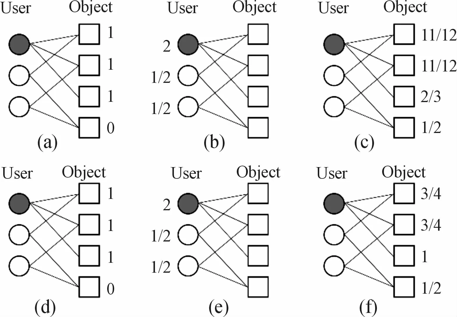
Fig.1 Transfer process in the bipartite graph with Prob S and HC；（a）（b）（c）correspond to Prob S；（d）（e）（f）correspond to HC

It is interesting to note that Zhou et al.［9］，who introduced a parameterθ（θ∈［0，1］），combined the above two algorithms to obtain a hybrid recommendation algorithm.The algorithm parameters can be adjusted under different application scenarios：

The equation represents HC whenθis 0，and ProbS whenθis 1.Specifically，whenθis 0.5，this algorithm can be seen as a combination of the cosine index and RA index，i.e.，CosRA：

CosRA integrates the benefits of the indices，resulting in excellent performance in both accuracy and diversity.

2.2 Real-timerecommendation algorithm based on time factor

Common recommendation algorithms incorporating the time factor include the timeliness-based recommendation algorithm（T algorithm）［29］and the recent degree increase algorithm［28］（DI algorithm）.Based on benchmark algorithms，these algorithms introduce the time factor to adjust resource allocation for the items on the recommendation list.Zhang et al.proposed a new measure，known as timeliness，of the popularity degree of the new or long-term items on the market.This algorithm emphasizes the timeliness of the items，which dictates the need to suppress the scores of outdated items and to increase the scores of popular items.Its definition is as follows：

Where iαis the time of occurrence of object set Uα；t0is the start time of the data set；and kαis the degree of itemα.This method can be used to effectively suppress the recommendation of outdated items and adjust their resource score：

WhereΔk′α（t，τ）is the degree increment of itemα after passing time intervalτto time t，i.e.，Δkα（t，τ）＝kα（t）-kα（t-τ）；kα（t）is the degree of itemα at time t.The resource score of the items can be influenced ifΔkα（t，τ）is zero；to avoid this，a very small value ofεis usually selected.In combination with the benchmark recommendation algorithm，the preliminary calculated resource score of the recommendationis first obtained and then incorporated with the time factor to obtain the final resource score，as shown below：

The reason why this method is outstanding is that the item popularity degree is an important reference factor during the evolution of the bipartite graph.

3 Real-time recommendation based on ComPI

3.1 Time-weight decay model

We found that items undergo complex and highly diversified development in recommendation systems.New items and new users are constantly emerging in a dynamically developing recommendation system.Items recommended by the system undergo a life cycle of forming，growth，maturing，recession，and becoming utterly obsolete on the market.Fig.2 shows the above product life cycle curve.However，there are many special product life cycle curves，including four special types of style，fashion，fad and scallop，as shown in the upper right corner of the Fig.2.The style-and scallop-type items grew slowly in the later stages of development.Most current recommendation algorithmsare overly focused on the recent item degree increase.It is easy to cause“marketing myopia”，that is，mistakenly believe that the item has reached the recession period and prematurely remove items that still have recommended value from the recommended list.This may cause items such as style-and scalloptype to be removed prematurely.For example，classic movies still have recommended value after a long time.

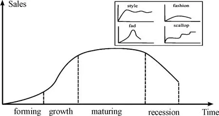
Fig.2 Product life cycle curve.The chart in the right upper corner shows the special product life cycles

In recommendation systems，not only the development time of the recommendation system but also the life cycle curve of the item must be considered，and combine the two to comprehensively measure the recommended value of the item.When making recommendations to users，similar items may be at different stages of development.Nevertheless，when considering the novelty of the items and user experience，items with higher comprehensive popularity are favored for the recommendation.Therefore，assigning weights to time to measure the development stage of an item is essential in recommendation algorithms.

How to allocate a reasonable weight to the time factor is a key issue.Since the volume of information in the recommendation system increases exponentially，an exponential-type time weight-decay model was proposed to analyze item popularity.Both the volume of information and the emergence of users were unpredictable or uncontrollable over continuous time.Also，during the collection process，missing values and outliers seemed inevitable.The discretization of continuous time into time intervals was performed by binning.This method could transform fluctuating data into several groups of stationary data，and the model became more stable after discretization，thus reducing the risk of overfitting of the model.Discretization also displayed strong robustness regarding outliers and could smooth out the data to reduce the influence of outliers on the overall performance.Depending on the start and end time of the data set，a time duration of thedata set was partitioned into n bins，which were successively denoted as T1，T2，T3，…，Tn.Then，the time-weight decay model was built using the exponential function.That is，the weight assigned to interval T1nearest to the latest time of the data set was 1；the weight assigned to interval T2was 0.5，and the weight assigned to interval T3is 0.25，and so forth.Therefore，the weight assigned was smaller for a time that was further away from the present，as shown in Fig.3.The time-weight decay model was defined as follows.The continuous time was partitioned into n bins，and the weight assigned to the i-thinterval was given by：

Fig.3 Time-weight decay model，with the data set partitioned into n bins and a weight assigned to each interval

3.2 Recommendation with ComPI

Item popularity was generally represented by the degree and time of occurrence of the item：the larger the degree and the later the occurrence of the item，the higher the item popularity and the higher the probability of recommendation.Here，based on the historical popularity of the item within the time interval，the probability of the item being recommended was predicted.The time-weight decay model divided a time duration into mutually independent intervals along the timeline.When a user selected a certain item，this event had only one interval to correspond to it.Events occurring within different intervals had no mutual impact on each other.These time intervals were treated as bins containing all of the items occurring within this interval.The probability of the itemαbeing randomly drawn from one of these bins was seen as the probability of the item being recommended.These“bins”composed a complete event groupΩ＝｛T1，T2，T3，…，Tn｝，where TiTj＝φ（i≠j，i，j＝1，2，3，…，n）；P（Ti）is the probability of the item being drawn from the bin denoted by Ti，hence：

Items were randomly drawn from these bins，and the event that the item drawn randomly from the bins is is denoted as B.The probability of occurrence of the item in each bin varied.The higher the occurrence frequency，the higher the ratio of the degree of this item in this interval to the total degree of this item，and hence the higher the popularity of this item in this interval.We let P（B｜Ti）be the probability of item occurring in the bin denoted by Ti：

Here，kiαis the degree of itemαin the bin Ti，and kαis the total degree of itemα.By using the formula for total probability，the probability P（B）of the itemα being drawn from these bins could be preliminarily estimated，i.e.，the probability of the item being recommended to the user was as follows：

As analyzed above，different weights were assigned to different time intervals，and they influenced item popularity to different degrees.By combining the total probability model and the time-weight decay model，a novel model based on ComPI was proposed.The algorithm mines the comprehensive popularity of items according to the active status.Thus，items with style-or scallop-type life cycle will not be eliminated from the recommendation list because of the insignificant recent growth rate.The macroscopic changes of the items in the bipartite graph were used to measure the popularity as it evolves，which was given by：

Where S（α）is the comprehensive popularity score of itemα；the higher the score，the higher the probability of the item being recommended；on the contrary，the lower the score，the smaller the probability of the item being recommended.This recommendation algorithm based on ComPI could effectively differentiate items with the same degree based on popularity.For example，consider two items with the same degree.The comprehensive popularity is higher for the one with a higher ratio of degree in the time interval assigned with a greater weight to the total degree of the item，and the comprehensive popularity is lower for the one with a lower ratio of degree in the time interval assigned with a smaller weight to the total degree of theitem.It can assign higher weights to items in the development period and lower weights to items in the recession period.

Based on ComPI，a real-time recommendation algorithm that integrated the benchmark bipartite-based recommendation algorithm was proposed.This novel algorithm was free from the influence of other factors and enabled a combination with any benchmark recommendation algorithm as needed.After obtaining the preliminary resource allocation resultfor item，the comprehensive popularity of items S（α）was introduced to correct the resource score of itemαand obtain：

Finally，the corrected f″（i）for user i was ranked in descending order，and the first L items were chosen to generate the final recommendation list.

4 Numerical experiments

4.1 Data description

Five open classical recommendation data sets incorporating time were used for experimentation，namely，two MovieLens data sets，two Netflix data sets and one E-commerce data set.The MovieLens data sets were classical data sets for testing recommendation algorithms and contained user rating data for movies provided by the GroupLens project of Minnesota University.According to the time interval of collection，the MovieLens-1M data set was the larger one，and MovieLens-100k was the smaller one.The rating range was［1，5］.Data with a rating below 3 were eliminated in this study.The Netflix data set came from the movie rental website and contained ratings given by about 4.8 million anonymous users on approximately 17 770 movies from December 1999 to December 2005.The rating range was also［1，5］，and data with ratings below 3 were eliminated.From the Netflix data set，two subsets were randomly drawn：one was the Netflix-10000 data set，comprising10 000 users and over 5 000 items；the other was Netflix-2000，comprising 1999 users and over 10 000 items.E-commerce is a transnational data set which contains all the transactions occurring between 01／12／2010 and 09／12／2011 for a UK-based and registered non-store online retail.After processing，the basic information for each data set was obtained and is shown in Table 1.

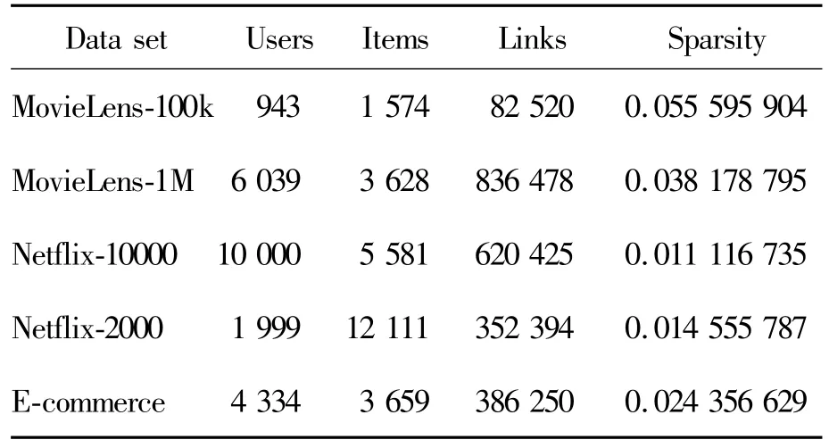
Table 1 Basic information of all data sets used in this study，including number of users，number of items，number of edges，and data sparsity

4.2 Data partitioning

We discussed the data partitioning methods in recommendation systems.A recommendation algorithm can be evaluated based on its ability to predict the connection between users and items in a network.Conventional methods for data partitioning usually involve a training set and test set.Generally，a data set is randomly partitioned into 10 parts via 10-fold crossvalidation；nine parts are used as training data，and one serves as the test data set.The training-to-test ratio can also be set to 8∶2 or 5∶5.This data partitioning scheme can effectively reduce error，although there are some disadvantages，such as the lack of time sequence logic.During the random drawing of data，the future behavior of users may be classified as historical behavior.In actual application，new items constantly appear in the data set.With the conventional data set classification method，some newly occurring items may be classified into the training set，whereas they are absent from the testing set.This data partitioning method was not suitable for the algorithm with the time factor.

Zhang et al.［29］proposed a data partitioning method based on time series.An appropriate time point was chosen after ranking the time series data.All of the data before this time point formed the training set；those after it formed the test set.Separate experiments were conducted repeatedly by moving the time point，and the training-to-test ratio was 50%-50%，60%-40%，and 70%-30%，respectively.The performance of the recommendation algorithm varied with the training-to-test ratio.Another data partitioning method incorporating the time factor was proposed by Vidmer et al.［28］.It was assumed that the timestamp of the entire data set was from 0 to Tm.A timestamp Tpwasrandomly selected，with the restriction Tp∈［0.8Tm，0.9Tm］imposed.The data from 0 to Tpwere chosen as the training set，and those from Tpto Tp＋Δp were selected as the test set.ParameterΔp represents the time span，as shown in Fig.4.

Fig.4 Data partitioning method proposed by Vidmer et al

As a result of varying features of the original datasets，the size of the test set may have been far larger than that of the training set.However，in a real-life setting，the data volume does not increase linearly over time.For example，the transaction volume at ecommerce websites usually increases abruptly on holidays or sale days.As shown in Fig.5，the data volume in the Netflix data set has grown exponentially over time.Therefore，Δp should be sufficiently long to allow a large number of items to be selected for the test set.However，Δp should not be too long either.

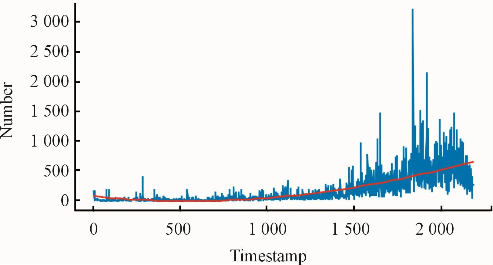
Fig.5 The data volume in the Netflix data set.The solid blue lines represent the number of data records at the corresponding time；the red dotted lines represent the overall exponentially increasing trend of data volume

Besides the logical time sequence of the experimental data，the growth features of the data also had to be considered in the experiment.While ensuring sufficient time sequence consistency was important，our main concern was the ability of the recommendation algorithm to predict network structural evolution within the existing historical data.The following data partitioning method was used：First，the data were ranked in chronological order；under a specific proportion，all of the data before the n-thdata instance formed the training set，and n to 10%*n（or 20%*n）data formed the test data.This partitioning method ensured that the timestamp of the test data was later than that of the training data and that the test set was of an appropriate size.Several groups of tests were conducted in the following scheme：The first 50%of data in the data set was used as the training set，and 50%-55%of the data was used as the test set；then，the first 60%of the data was used for training，and 60%-66%was used for testing.Next，the first 70%of the data was used for training，and 70%-77%was used for testing；then，the first 80%of the data was used for training，and 80%-88%was used for testing.Finally，the first 90%of the data was used for training，and 90%-99%was used for testing.

4.3 Evaluation indicators

The performance of a recommendation system is usually evaluated in terms of accuracy，diversity，and novelty.In this study，four performance indicators，namely，AUC，precision，MAP，and recall，were chosen as accuracy measures.AUC refers to the area under the ROC curve［31］.Generally speaking，AUC is a measure of whether the current ranking is optimal.When calculating AUC，the edges in the test set are compared one by one against those in the recommendation list.If the ranking of the edges（or weight）in the test set is higher than that of the edges（or weight）absent from the test set，then N′＋1；if the two are the same，then N″＋1.The larger the AUC，the higher the probability that the objects randomly chosen are ranked higher than those not randomly chosen，and hence there is a higher accuracy.AUC is given by：

Where m is the number of users.Here the means of all users were taken.The other three accuracy indicators were closely related to the length of the recommendation list，namely，MAP（mean average precision）［32］，precision，and recall［33］.MAP is a standard single-number measure for comparing search algorithms in terms of overall ranking precision.This indicator can be understood in three parts，namely，Precision，AP（average precision），and MAP（mean average precision）.

1）Precision refers to the accuracy of the recommendation list.It is defined as the proportion of the items chosen by the user in the recommendation list and reflects the accuracy of the recommendation.Pre-cision is defined as：

Where di（L）is the number of shared items in the recommendation list with length L and the test set for user.Recall is another important indicator usually used in tandem with precision.Recall represents the proportion of accurate or relevant information being detected.It is the ratio of the number of items on the recommendation list for the user to the total number of items in the test set.The definition of recall is given below：

Where D（i）is the number of items in the test set.

2）APis the average precision，which is mathematically defined as

Here，rsis the ranking of the s-thitem in the recommendation list，and.rs∈［1，L］APis very sensitive to ranking；the higher the ranking of the item，the larger the AP.

3）MAP，or mean average precision，is the calculation of the mean AP of several validation individuals and measures the accuracy of the algorithm at the general level.The larger the MAP，the higher the accuracy.The definition of MAP is given below：

According to the formula above，MAP is closely associated with the ranking in the recommendation list.The 10-fold cross-validation is usually used for data partitioning for conventional recommendation algorithms.Since data partitioning in that case is completely random，poor time sequence logic is likely to occur.As a result of this，the data that should have been ranked lower on the list can be mistakenly ranked higher，and vice versa.Therefore，the reliability of MAP can be improved by incorporating the time factor into the recommendation algorithm.Ranking the data in chronological order and performing a reasonable division of the data set can ensure the logical progression of the time series.For this reason，MAP incorporating the time factor is more convincing.

Novelty and diversity of recommendations have become an important part of recommendation evaluation［34］.From the user’s perspective，the novelty and diversity are direct sources of user satisfaction.How to obtain a balance between the accuracy，diversity，and novelty is another research focal point［35］.Diversity of recommendation refers to the number of types of items in the recommendation list.It is usually measured by intra-similarity［36］，given by：

Cosine similarity between items in the recommendation list for the target user is used as the similarity indicator.is the cosine similarity between itemsαandβ in the recommendation listwith a length of L.The smaller the intra-similarity，the larger the number of types of items recommended in the list and the higher the diversity.The Hamming distance［37］is another commonly used measure of diversity.In actual applications，the mean Hamming distance of all users is usually taken.Here，C（i，j）＝｜is the number of identical items in the recommendation list for user i and j user.The greater the Hamming distance，the higher the diversity：

Novelty can be understood in terms of the difference between the present and the past.It is only subtly different to the concept of diversity.The novelty indicator is a quantification of the ability of the algorithm to generate unpopular or unexpected results［38］，given by：

Where kαis the degree of itemαin the recommendation listfor user i；the smaller the value，the higher the novelty，and the better the feeling of freshness and user experience.

5 Experimental results

We used AUC，precision（P），recall（R），MAP，Hamming（H），intra-similarity（I），and novelty（N）as evaluation indicators.Comparative experiments were conducted between the different algorithms in four different ways：（1）comparison between the combination of the ComPI-based recommendation algorithm with the conventional benchmark algorithms and the use of the original algorithms alone；（2）comparison between the combination of the ComPI algorithm and conventional benchmark algorithms and that of thetimeliness-based algorithm（T algorithm）and conventional benchmark algorithms；（3）comparison between the combination of the ComPI algorithm and conventional benchmark algorithms and that of the degree increment（DI）algorithm and conventional benchmark algorithms；and（4）comprehensive comparison between all of the above-mentioned algorithms incorporating the time factor（T algorithm，DI algorithm，and ComPI algorithm）.The results of the four experiments are presented below.

5.1 Comparison with the benchmark algorithm

Tables 2 shows the results of the combination of the ComPI algorithm with each of the conventional recommendation algorithms.Here，three benchmark recommendation algorithms，namely，HC，ProbS，and Cos-RA，were run on four data sets，namely，MovieLens-100k， MovieLens-1M， Netflix-10000 and E-commerce.Five independent experiments were carried out using the data set division method described above，and the averages were taken.The length L of the recommendation list was set to 50.

According to the Table 2，the ComPI algorithm combined with the benchmark algorithm was improved significantly in terms of accuracy and diversity.For the ComPIalgorithm，the binning factor was set to n＝5，n＝5，n＝60 and n＝25 for the four data sets，respectively.In general，the accuracy indicators showing a significant increase were AUC，recall，and MAP，and the indicator with a mild increase was precision.As to diversity，both intra-similarity and novelty were significantly improved.For the two MovieLens data sets，which had a smaller data volume but higher density，the diversity indicator was improved more apparently while accuracy improvement was ensured.After the ComPI algorithm was combined with the HC algorithm with greater diversity，the novelty indicator decreased by about 50%.For the Netflix-10000 data set，which had a larger data volume but lower density，the accuracy improvement was even more dramatic.After the ComPI algorithm was combined with the CosRA algorithm，the highest precision reached 0.042，which was about 18%higher；the highest MAP was 0.0889，with an improvement of 52.93%.The ComPI algorithm fully considered the development stage of the items，and suppressed the scores of items entering the recession period，which effectively improved the performance of the benchmark algorithm.

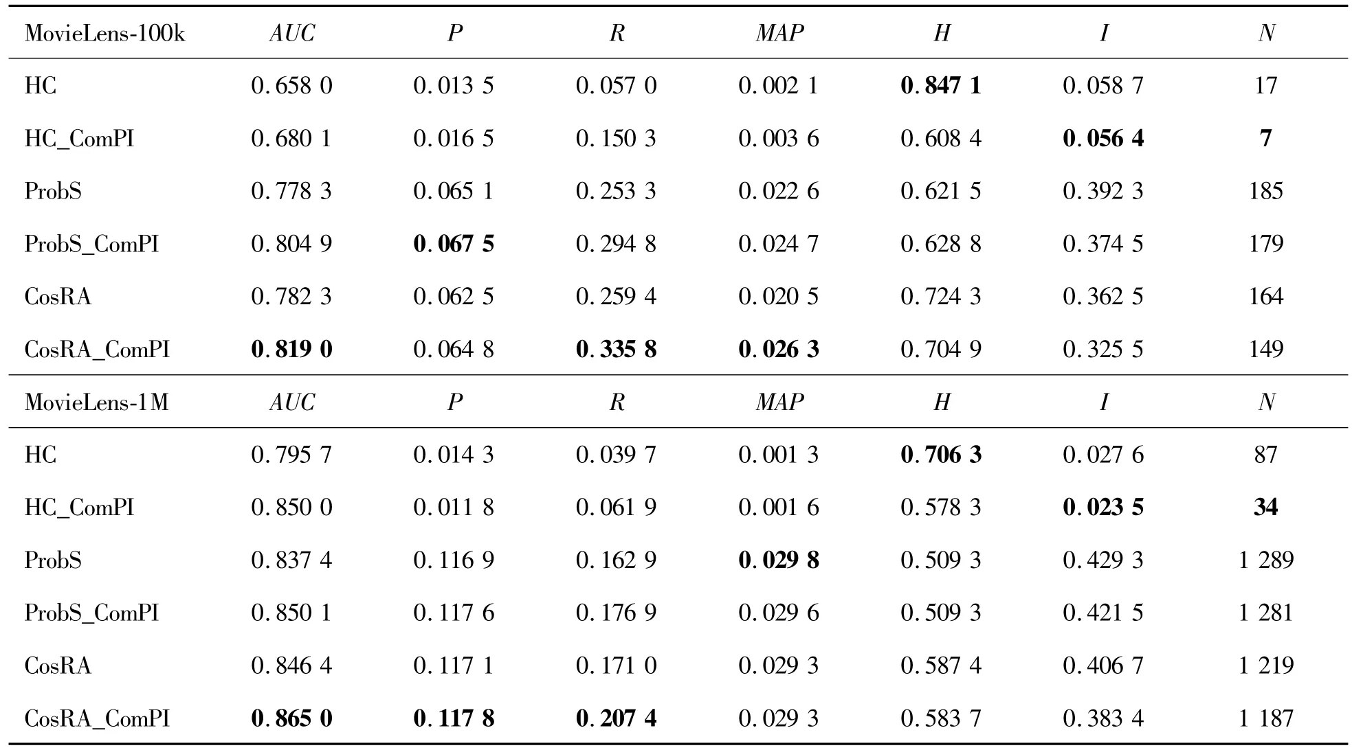
Table 2 Experiments for the MovieLens-100k，MovieLens-1M，Netflix-10000 and E-commerce data sets.Suffix ComPl represents the incorporation of the ComPl algorithm into the benchmark recommendation algorithms

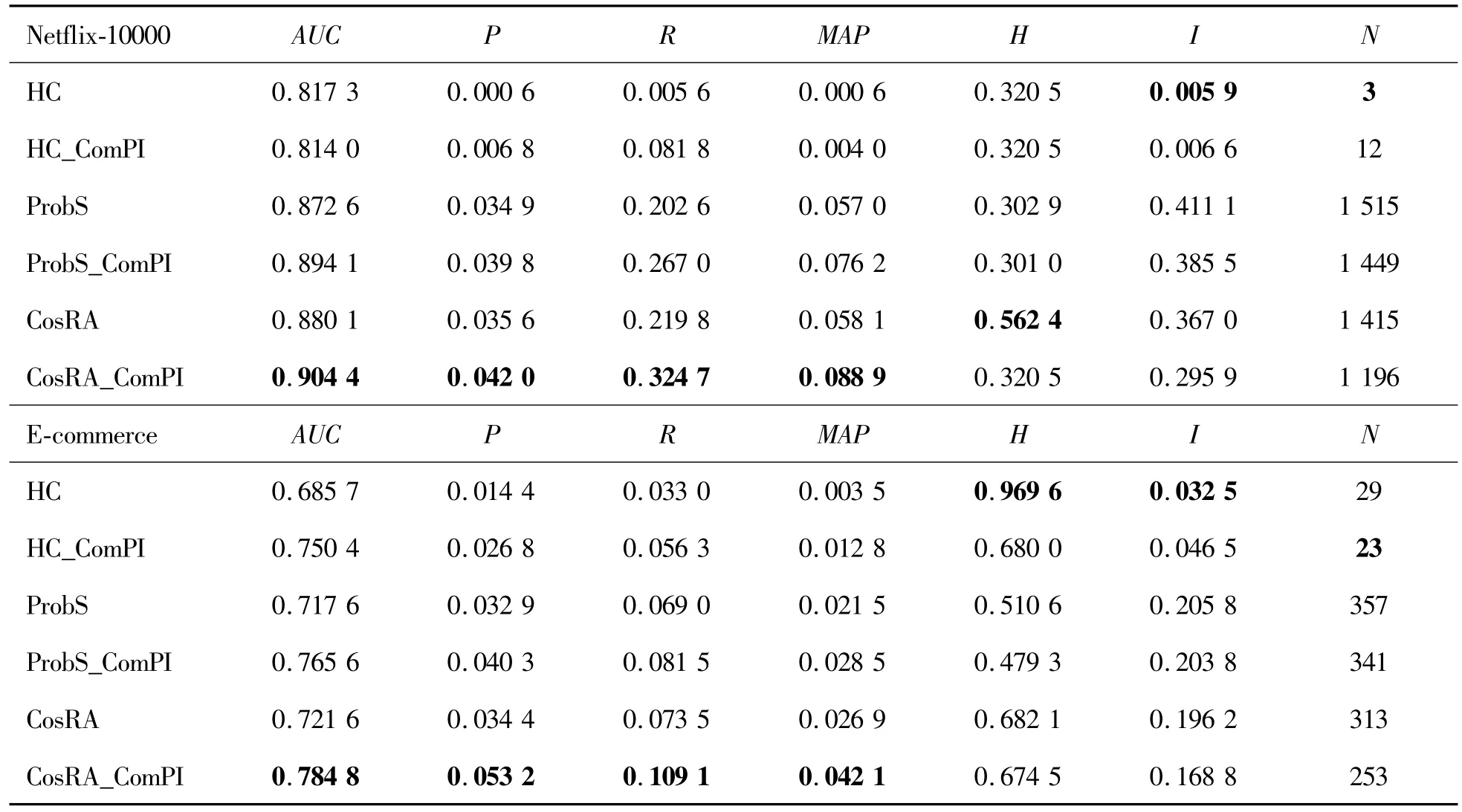
Continued Table

5.2 Comparison with the T algorithm

We further compared the combination of the ComPI algorithm and conventional benchmark algorithms and that of the T algorithm and conventional benchmark algorithms.To carry out a more fair and accurate comparison，the data set was partitioned into test and training sets using the method proposed for the T algorithm.The MovieLens-1M and Netflix-10000 data sets were used for the experiments.Five subsets of the training set were partitioned in ascending order of size for independent experiments.The time interval n for the ComPI algorithm was set to 5 and 60，respectively.The length of the recommendation list was set to 50.In Fig.6 and Fig.7，the benchmark algorithms are represented by green dotted lines，the ComPI algorithm by red solid lines，and the T algorithm by blue dotted lines.

For the MovieLens-1M data set，the size of the training set increased from 50%to 90%.The precision and MAPof all algorithms first increased and then decreased.Recall showed an increasing trend，whereas intra-similarity showed a decreasing trend，as shown in Fig.6.The precision，recall，MAP，and intra-similarity of the ComPI algorithm，combined with the conventional benchmark algorithm，were generally similar to those of the T algorithm combined with the conventional benchmark algorithm.However，these indicators were improved most significantly for the benchmark algorithms using the ComPI algorithm when the size of the training set was 50%.For this size of training set，the recall was significantly improved with CosRA，and MAPwas higher with HC.Moreover，the intra-similarity was higher for the algorithms based on ProbSand CosRA.As shown in Fig.7，there was only a moderate performance improvement for the MovieLens-1M data set，but the ComPI algorithm combined with the conventional benchmark algorithm showed excellent performance for the Netflix-10000 data set.As the size of the training set changed，the ComPI algorithm combined with the conventional benchmark algorithm consistently outperformed the T algorithm，whether in accuracy indicators or diversity indicators.Taken together，for the data set partitioned by the time factor，the ComPI algorithm was able to more comprehensively consider the popularity of the items and therefore resulted in a significant improvement in diversity and novelty while ensuring accuracy.When recommending the recently popular items for the users，items with a greater degree were not excessively recommended，and nor were those with a smaller degree excessively suppressed.The ComPI algorithm has more accurate weight distribution for items with different life cycles.

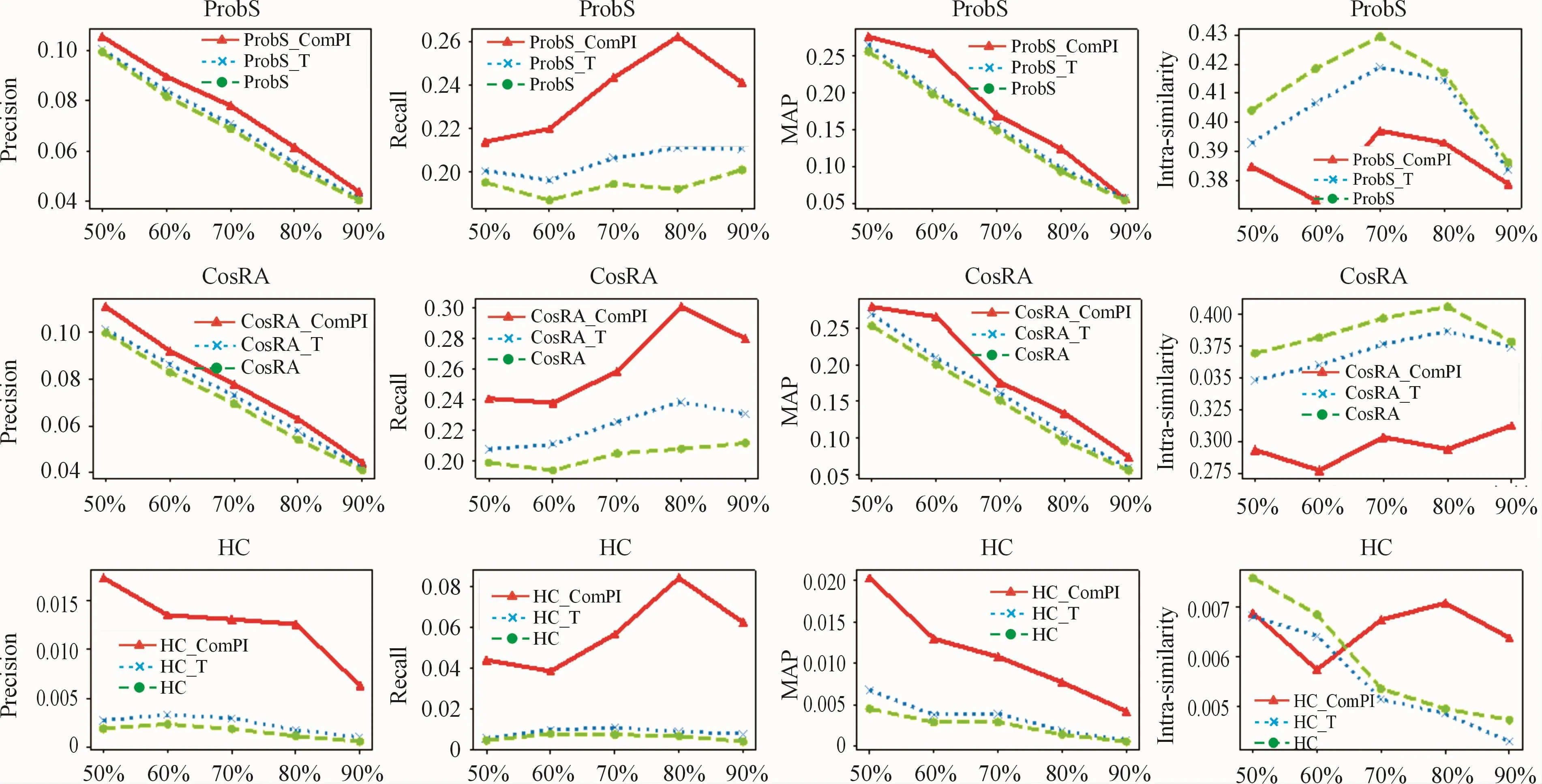
Fig.7 Experiments for the Netflix-10000 data set

5.3 Comparison with the DI algorithm

As above，a comparison was performed between the combinations of the ComPI algorithm and different benchmark algorithms and those of the DI algorithm and different benchmark algorithms.The Netfilx-2000 data set and the partitioning method described in the article for the DI algorithm were used.The time interval chosen for this data set was 1 d.The training set was composed of the data at 1 d after the timestamp of the training set.The ComPI algorithm and DI algorithm were applied to ProbSand CosRA.The length of the recommendation list was set to 50.

For the Netflix-2000 data set，the two algorithms had the best performance when the binning factor nwas 80 for ComPI and the parameterτwas 10 for DI.According to Table 3，the DI algorithm combined with ProbS outperformed the ComPI algorithm combined with ProbS.The former had the highest values of recall，MAP，intra-similarity，and novelty indicators，especially recall and MAP.The ComPI algorithm improved the performance of ProbS to a certain degree，but unlike the dramatic improvement in diversity with the DI-based algorithms，the former showed a more moderate improvement.The DI algorithm combined with CosRA was inferior to the ComPI algorithm combined with CosRA.The latter achieved the best values of AUC，precision，MAP，and novelty，whereas the former was only improved significantly in recall and intra-similarity.As seen from the above，the ComPI algorithm combined with any benchmark algorithm achieved a stable performance improvement.This effect did not fluctuate dramatically with the type of benchmark algorithm.The ComPI-based algorithms were more suitable for recommending novel items to users，and the DI algorithm highlighted the microscopic aspects of network growth.In contrast，the proposed ComPI algorithm highlighted the overall trend of the items in the network，considering item popularity both at present and in other time periods.Compared with the DI algorithm，the ComPI algorithm can take into account the items with style-and scallop-type life cycles and guarantee their scores.It was not entirely focused on recommending recently popular items，which improved the problem of“marketing myopia”in recommendation systems.Therefore，this method could improve the accuracy.

Table 3.Experiments for the Netflix-2000 data set.Suffixes Dl and ComPl represent the algorithms combined with Dl and ComPl，respectively.The parameterτwas set to 10 for the Dl algorithm，and the binning factor n was set to 70 for the ComPl algorithm

5.4 Comprehensive comparison of algorithms considering the time factor

In the experiments above，the ComPI algorithms combined with different conventional benchmark algorithms were compared against the T and DI algorithms combined with these conventional benchmark algorithms on different data sets that were partitioned by the methods in literature.To better determine the performance of each algorithm under different conditions，the DI，T，and ComPI algorithms were combined with CosRA and tested on data sets that were partitioned by the method proposed in the present study.The MovieLens-100K，Netflix-10000，MovieLens-1M，and E-commerce data sets，which differed most dramatically in data characteristics，were chosen for the experiments.The length，L，of the recommendation list was set to 50.As shown in Table 4.

For the MovieLens-100K data set，the DI algorithm combined with CosRA had the best performance when the time interval，τ，was 1 000 000；the ComPI algorithm combined with CosRA had the best performance when the binning factor，n，was 5.The ComPI algorithm combined with CosRA had the best performance for AUC，recall，and MAP.This algorithm outperformed the methods based on the DI and T algorithms regarding the accuracy.For the Netflix-10 000 data set，the DI algorithm combined with CosRA had the best performance whenτwas 10 000；the ComPI algorithm combined with CosRA had the best performance when the n was 60.For the E-commerce data set，the DI algorithm combined with CosRA had the better performance whenτwas 1 000 000；the ComPI algorithm combined with CosRA had the better performance when the n was 25.For the MovieLens-1M data set，the DI algorithm combined with CosRA had the better performance whenτwas 10 000；the ComPI algorithmcombined with CosRA had the best performance when the n was 5.Among the three algorithms incorporating the time factor，the ComPI algorithm improved the accuracy of the benchmark algorithm most significantly，with AUC achieving 0.9045.The highest precision was 0.042；the recall was improved to 0.324 7，and the MAPwas0.0889.The DI-based algorithm had the best performance for diversity.The comparative experiments indicated that the ComPI algorithm achieves a more general and stable improvement of the performance of the benchmark algorithms.Also，the ComPI algorithm applies to the data sets with various growth characteristics and displays high robustness.The performance of the algorithm does not vary greatly due to changes in data partitioning methods.Its demonstrated ability to improve the performance of the benchmark algorithms is particularly significant for data sets with a large data volume and sparse density，as this algorithm fits the application scenarios more closely.

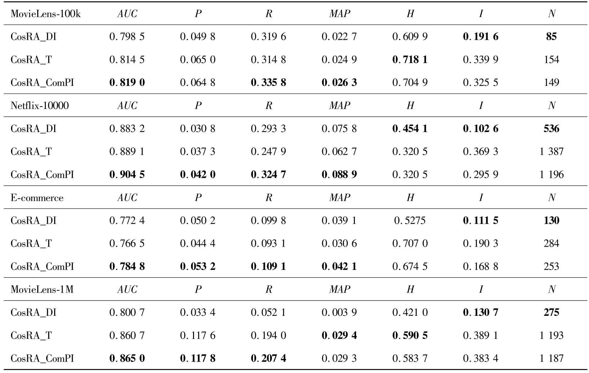
Table 4.Experiments for the MovieLens-100k，Netflix-10 000，E-commerce and MovieLens-1M data sets.Suffixes Dl，T，and ComPl represent the Dl，T，and ComPl algorithms，respectively

In general，items with different life cycles have different characteristics in time and degree.Items with style-and scallops-type have a long time span and a large degree in recommendation systems；items with fashion-and fad-type have a short time span but a large degree.Taking the experimental results on MovieLens-100k and analyze the items recommended by the three algorithms，as shown in Fig.8.The horizontal axis is the time span of the item in the training set（timestamp of the last occurrence of the item minus timestamp of the first appearance of the item），the vertical axis is the degree of the item.Items recommended by ComPI algorithm and T algorithm are represented by red dots and green squares，respectively.It can be found that they mainly recommend items with a long time span.The ComPI algorithm also fully considers items with a short time span but high recommendation value，as shown in the lower side of the Fig.8.The DI algorithm focused on the item recent degree increase and assigned a higher score to items with a smaller degree，as shown by the blue triangles in the lower right corner of the Fig.8.Therefore，the diversity of the DI algorithms is better.In summary，the ComPI algorithm can more accurately measure the comprehensive popularity of items according to the item development，which has higher accuracy.

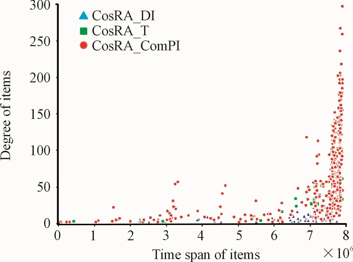
Fig.8 ltems recommended by the Dl，T，and ComPl algorithms

6 Experimental analysis

6.1 Influence of time weight

In the ComPI model，continuous time was discretized，and the binning factor，n，was introduced to adjust the time weight.Data sets with different time spans had different n values.To analyze the influence of time weight on the ComPI algorithm，a continuous time-weight decay model C（t）and discrete timeweight decay model were built and compared.The former mapped the timestamp to the interval［0，5］，i.e.，C（t）＝et.Parameter t is the value of the timestamp of the item mapped to the interval［0，5］；C（t）is the time weight of the item at time t.All of the time weights assigned to a specific item for their occurrence were added up to obtain the final recommendation score S′（α）＝∑C（t）.Experiments were carried out using the MovieLens-100k and Netflix-10000 data sets.The binning factors were set to n＝5 and n＝60，respectively，for the ComPI algorithm，and the length of the recommendation list was 50.The experimental results are shown in Table 5.

Table 5.Experiments for the MovieLens-100k and Netflix-10000 data sets.Suffix EXP is attached to the continuous model，and binning to the discretized model

As shown in Table 5，the continuous time-weight decay model was inferior to the discrete time-decay model in both accuracy indicators，such as precision，recall，and MAPand in diversity.The possible reason was that the time-weight allocation with the continuous model is consistently an exponential function，and therefore the weight assigned was more fixed.However，in the discrete time-weight decay model，the time weight constantly changes with the bin number；the wider the bin，the smaller the difference in weight.As analyzed above，the discrete time-weight decay model can assign a more reasonable time weight and is more appropriate for the ComPI algorithm.

6.2 Influence of bin count

As shown above，the binning factor，n，in the timeweight decay model seemed to exert an inevitable influence on algorithm performance.During the binning process，a bin number that was too small led to an absence of significant difference between weights assigned to different time intervals；if n was too large，the weight decayed too rapidly.Several experiments investigating the change of n within a specific range showed that the accuracy indicators of the ComPIalgorithm first increased with increasing n and then stabilized；likewise，the diversity indicators first increased with increasing n，then decreased and finally stabilized.The ComPIalgorithm was combined with CosRA and tested on the Netflix-10000 and MovieLens-1M data sets.As shown in Fig.9，the range of n for the Netflix-10000 data set was［0，100］.Precision and recall showed roughly the same increasing trend as n increased.When n was 50，the precision and recall stabilized at 0.042 and 0.32，respectively.The diversity indicators novelty and intra-similarity also approached 1 195 and 0.295，respectively，after n increased to50.As shown in Figure 10，the value range of n for the MoiveLens-100k data set was［1，15］.After n＝5，the precision began to fluctuate around 0.064 5.The recall increased rapidly before n＝5 and then stabilized at about 0.325.Intra-similarity and novelty also decreased with increasing n，showing an overall decreasing trend until gradual stabilization towards the end.Also，when n in the two experiments approached infinity，the accuracy indicators of the ComPI algorithm gradually decreased，while the diversity indicator novelty decreased.The bin count had a significant impact on the ComPI algorithm.Within a specific range，the diversity and accuracy indicators of the algorithm first increased and then stabilized with increasing n.In actual use，an appropriate bin number should be selected according to the time span of the data set.

Fig.9 Change in precision，recall，novelty，and intra-similarity with increasing n for the Netflix-10000 data set

Fig.10 Change in precision，recall，novelty，and intra-similarity with increasing n for the MovieLens-100k data set

6.3 Influence of data characteristics

The performance of the ComPI algorithm was the best for the Netflix data sets among all of the data sets.The growth of the data sets could be described as S-shaped curves，J-shaped curves or liner.Fig.11 shows the variation in the total degree of items in the three data sets with time.The MovieLens-1M data set showed an apparent S-shaped growth pattern，the MovieLens-100k data set showed a linear growth pattern，and the Netflix data set showed an apparent J-shaped growth pattern.The data with S-shaped growth were more stable on the whole，with fewer new items，and the variation of the trend of the items was similar.J-shaped growth，also known as exponential growth，was associated with a large number of new items in the data set as well as a higher diversification among items.According to the experiments in the previous section，the ComPI algorithm improved the performance of the conventional benchmark algorithm more significantly on the MovieLens-100k data set with linear growth than on the MovieLens-1M data set with S-shaped growth.Specifically，when the training-to-test ratio in chapter 5.2 was 50%：50%，the training set exhibited exponential growth on the whole.The ComPI algorithm displayed a dramatic performance improvement as compared with the other four sub experiments.For the Netflix data set，the performance of the ComPI algorithm was improved significantly in accuracy，diversity，and novelty.

Fig.11 Variation in the number of items in the data set over time（summation of the number of occurrences）.

Generally speaking，items with an S-shaped growth are at the recession stage，and the market demand for such items is far less than that for items in the growth stage.Therefore，the recommendation scores of such items should be suppressed.Items with a J-shaped growth are generally at the growing stage，and the market demand for such items is high.Therefore，the recommendation scores of such items should be increased as appropriate.The S-shaped growth data set is suitable for testing the performance of the algorithm without the time factor，while for testing the algorithm with the time factor，selecting the J-shaped growth data set can more realistically reflect the algorithm performance.Data sets with a J-shaped growth can more realistically reflect the constant emergence of new users and new items in the recommendation system.They are closer to reality and of higher practical value.Researchers should pay considerable attention to improving the algorithm performance on data sets with J-shaped growth.According to the results from chapter 5.4，it was easy to see that the T，DI，and ComPIalgorithms differed little regarding data with S-shaped growth.However，on data sets with J-shaped growth，the ComPI algorithm outperformed all of the other algorithms.Generally speaking，the ComPI algorithm applies to various types of data sets，especially on data sets with exponential growth.This algorithm is closer to reality and of high practical value.

6.4 Time information and resource allocation

The resource scores and time information of the items were further analyzed，with the following findings：（1）The items recommended by most of the algorithms accounted for only about 30%of the total items；（2）the recommended items were mostly those with larger degrees；（3）most of the recommended items had recent time information.The resource scores of each item in all of the recommendation lists were summed，as were the timestamps of each item.The relationship between the two factors was analyzed.Fig.12，（a），（b），（c），and（d）show the performance of the CosRA algorithm，CosRA_ComPI algorithm，HCalgorithm，and HC_ComPIalgorithm on the MovieLens-100k data set，respectively（the binning factor，n，in the ComPI algorithm was 5）.The red dots represent the items recommended to the users.The blue triangles represent the items not recommended by the algorithms.The pie chart in the right upper corner shows the ratio of the number of recommended items（red dots）to that of the non-recommended items（blue triangles）.

The CosRA algorithm had a higher accuracy，and the time information scores of the recommended items were proportional to the resource scores of the recommendation；moreover，the recommended items only accounted for about 30%of the total items，as shown in（a）.For CosRA_ComPI，the recommended items accounted for about 30%of the total items.The time information of the recommended items was roughly proportional to the resource scores.The distribution was sparser as compared with（a），and the time information scores of some items were lower，although the recommendation scores were higher.However，for other items，the time information scores were higher，while the resource scores were lower，as shown in（b）.Diversity was prioritized in the HCalgorithm，and the resource scores of the items were inversely proportional to the time information scores.The HC algorithm favored items with smaller degrees，and the recommended items accounted for about 70%of the total items，as shown in（c）.As compared with the HCalgorithm，the number of recommended items decreased with HC_ComPI.The recommended items accounted for about 30%of the total items，and those with smaller degrees were favored，as shown in（d）.The HC_ComPIalgorithm had higher accuracy and diversity compared with the HC algorithm，and the number of recommended items was reduced（as found in chapter 5.1）.

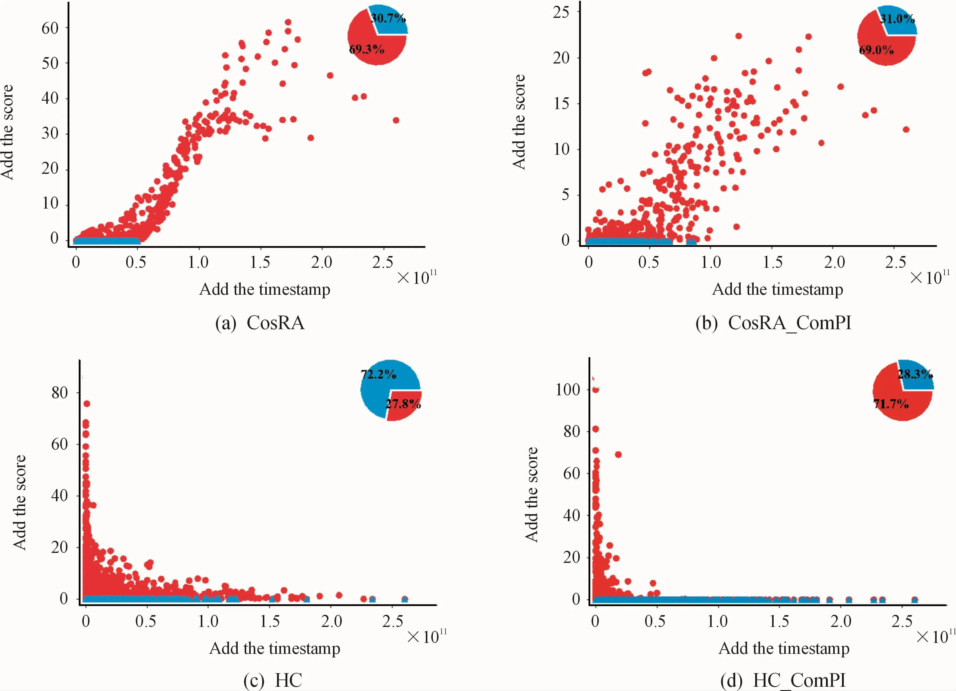
Fig.12 The resource score and time information score of each item in recommendation algorithm.（a）Cos RA algorithm；（b）CosRA_ComPl algorithm；（c）HC algorithm，and（d）HC_ComPl algorithm

Taken together，the recommendation algorithms with higher accuracy favored the recently popular items，and the recommended items accounted for about 30%of the total items.The proposed ComPI algorithm reasonably allocated time weights and resource scores and considered the comprehensive popularity of items，which improved the diversity and accuracy of the recommendations.

7 Conclusion

The time factor was introduced into the recommendation system to mine the development rules and comprehensive popularity of items.The macroscopic changes of items in the bipartite graph were placed at the center，and ComPI was prioritized.Discretization of a time duration was achieved by binning，and the timeweight decay model was built to reasonably allocate time weights to different intervals.The ComPI model measured the recommended value of items based on the development stage of the product life cycle.It can effectively distinguish between recession items，growth items and popular items，etc.，and solved the problem of“marketing myopia”in recommendation systems.Then，the real-time recommendation approach based on ComPI was detailed.The proposed ComPI algorithm was tested on real data sets，and the experimental results indicated that the ComPI algorithm has the following benefits：（1）Good universality：The ComPI algorithm can be applied to any benchmark recommendation algorithm and effectively improve their performance；（2）High stability：The algorithm displays excellent performance on data sets that have complex growth features and are partitioned in different ways.The ComPI algorithm applies to recommender systems with a large data volume，sparsity，and exponential growth features；（3）Strong robustness：The ComPI algorithm can stably improve the performance of the benchmark algorithms，regardless of the specific type of benchmark algorithm.（4）Flexibility and adjustability：The binning factor n can be changed as needed to adjust the time-weight flexibly.We also found that the growth of data volume has three types：S-shaped，J-shaped and linear.Data sets with a J-shaped growth should be paid more attention when testing the algorithm performance.Furthermore，the growth characteristics of data also have a certain impact on data division.The real-time recommendationalgorithm based on ComPIfully considers the popularity of items on the market both at present and in the past by incorporating the time factor.It can study the development process of items，optimize the users’recommendation lists，and effectively solve the problems of data sparsity，cold start and“marketing myopia”in recommendation systems.In addition，the ComPI model can also help to study the evolution process of network topology，and can be applied to network related fields，such as link prediction and network evolution.In future work，other information such as user interests，item labels and natural computation will be incorporated into the ComPI algorithm for improvement.