ASYMPTOTIC DISTRIBUTION IN DIRECTED FINITE WEIGHTED RANDOM GRAPHS WITH AN INCREASING BI-DEGREE SEQUENCE∗

Department of Statistics,South-Central University for Nationalities,Wuhan 430074,China

E-mail:jingluo2017@mail.scuec.edu.cn

Hong QIN

Department of Statistics,Zhongnan University of Economics and Law,Wuhan 430073,China,

E-mail:qinhong@mail.ccnu.edu.cn

Zhenghong WANG

Department of Statistics,South-Central University for Nationalities,Wuhan 430074,China

E-mail:wzh@mail.scuec.edu.cn

Abstract The asymptotic normality of the fixed number of the maximum likelihood estimators(MLEs)in the directed finite weighted network models with an increasing bi-degree sequence has been established recently.In this article,we further derive the central limit theorem for linear combinations of all the MLEs with an increasing dimension when the edges take finite discrete weight.Simulation studies are provided to illustrate the asymptotic results.

Key words Central limit theorem; finite discrete network;increasing number of parameters;maximum likelihood estimator

1 Introduction

Many statistical models have been developed to understand the generation mechanism and structures of networks(see[1,11,20,22]for recent review),with applications in authoring networks[17],company board networks[2],actor movie networks[23],community networks[21],and sexual contact networks[9].However,the non-standard structure of network data poses new challenges for statistical analysis,especially for asymptotic theory[10].

The degree sequences is one of the most important graph statistics and was extensively studied(see[3,5,6,13,19,29]).One natural approach for modeling the degrees is to put them as sufficient statistics for exponential family distributions on graph according to Koopman-Pitman-Darmois theorem([8,15,18]).The asymptotic properties of the maximum likelihood estimators(MLEs)have been little known until recently.As the number of parameters goes to infinity,the MLEs were proved to be uniformly consistent by[7]in the β-model;[26]established its asymptotic normality.When the edges take the binary,continuous and infinite discrete values,[24]established the uniform consistency and the asymptotic normality for a fixed number of the MLEs in directed exponential random graph models.[16]further derived a central limit theorem for linear combinations of all the maximum likelihood estimators with an increasing dimension.However,the finite discrete weight is not considered in their work.This case is also common in network data.For example,[12]recorded several social networks with vertices denoting academics joining in an experiment on computer mediated communication and the directed edges denoting the acquaintance information that were coded as the discrete values 0,···,4.A natural question appears.Is there similar results for a diverging number of the MLEs? This article aims to solve this problem.

In this article,we further establish a central limit theorem for a linear combination of all the MLEs with an increasing degree sequence when the edges take finite discrete weight,built on the work of[27].Obviously,the previous results on the fixed number of the MLEs is one specific case of the latter.Simulation studies and a data example are provided to illustrate the asymptotic results.

The rest of this article is organized as follows.In Section 2,we describe the finite discrete weighted network models and lay out the asymptotic result.Simulation studies are given in Section 3.Some further discussion is devote to Section 4.All proofs are given in Section 5.

2 Main Results

here Z(α,β)is the log-partition function,and α =(α1,α2,···,αn)⊤and β =(β1,β2,···,βn)⊤are parameter vectors.The αiquantifies the effect of edge connecting to vertex i and the βjquantifies the effect of edge connecting to vertex j.This model can be viewed as a generalization of the p1model by[14]without the reciprocity to weighted edges,and as a directed version of the β-model.Hereafter,we will refer to model(2.1)as the p0model,where the subscript “0”means the simpler model than the p1model.

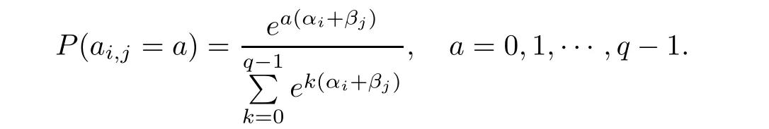
By(2.1),it can be shown that the probability mass function of aijis

The likelihood equations are

Here,the approximated inverse is used for representing the linear combination of all the MLEs as a function of the linear combination of all the degrees with the coefficientsandDetails are given in Section 5.Consider the following condition:

•A2

Theorem 2.1If condition A1 and A2 hold,as n→∞.Then,

is asymptotically normal with mean 0 and variance

Remark 2.2By choosing special cases of the sequencewe can obtain the central limit theorem for any combinations of fixed number of MLEs or a linear combination with a growing number of the MLEs.For example,if let(λk+1,λk+2···)=(0,0···)with a fixed k,then the theorems cover the results of[27].And let all κj=0,we get the central limit theorems for the linear combination of the estimators of the out-degree parameter vector,that is,

3 Numerical Studies

In this section,we will evaluate the asymptotic result in Theorems 2.1 through numerical simulations and a real data example.

3.1 Simulation studies

For the coefficient sequence,we set,whose absolute sum converges.Following[27],the parameter settings in simulation studies are listed as follows.Let

and considered four different value 0,log(log(n)),log(n)1/2,log(n)for L.For β,leti=0,1,···,n−1 andby default.Note that by Theorems 2.1,the quantile-quantile(QQ)plot the empirical distributions of

against the standard normal distribution were drawn to evaluate the asymptotic approximation.We ran 10000 simulations for each scenario.

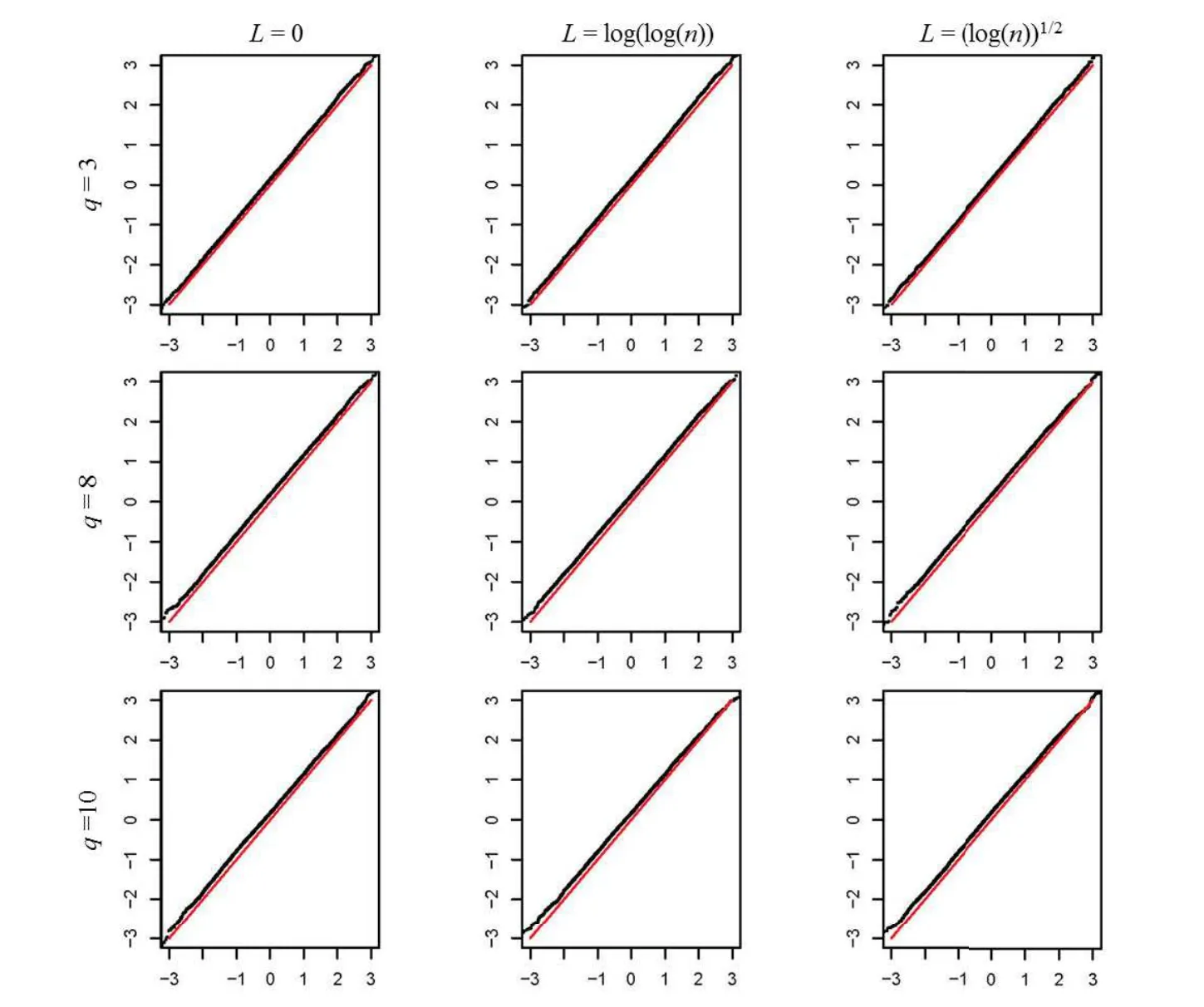
Figure 1 The QQ-plots(n=100,q=3,8 or 10)

Figure 2 The QQ-plots(n=200,q=3,8 or 10)

We simulated two value 100 and 200 for n and three values 3,8,and 10 for q.When L=log(n),the MLE in the case of q=3,8 and 10 failed to exist with 100% frequencies.Therefore,the QQ plots were not available under these cases.This also demonstrated the previous findings of[27].On the other hand,when L=log(log(n)),the frequencies that the MLE did not exist are 9% ,8% ,5% for n=100 in the case of q=3,8,and 10,respectively.For n=100,200 and L=log(n)1/2,the frequencies that the MLE did not exist are 28.97% ,3.17% in the case of q=3;For n=100,200 and L=log(n)1/2,the frequencies that the MLE didn’t exist are 27.91% ,3.12% in the case of q=8;For n=100,200 and L=log(n)1/2,the frequencies that the MLE did not exist are 28.2% ,3.17% in the case of q=10.In other setting,we did not observe the non-existence of the MLE.

The QQ-plots for two value n=100 and n=200 and three values 3,8 and 10 for q are shown in Figure 1 and Figure 2,separately.The horizontal and vertical axes are the theoretical and empirical quantiles,respectively.The gray lines correspond to the reference line y=x.In the first of Figures 1 and 2,the sample quantiles coincide with theoretical ones very well.On the other hand,in the second and third rows,the approximation of asymptotic normality are also good when L=0,log(log(n))while there is notable derivations when L=log(n)1/2.

For the fixed L and q,the mean value of the formula

increases with the increase of n in Table 1.And then the variance have similar trend.

Table 1 Themeans and their variances(in parentheses)

Table 1 Themeans and their variances(in parentheses)

cases L=0 L=log(log(n)) L=(log(n))1/2 n=100,q=3 0.206(1.471295) 0.215(1.471295) 0.181(1.471295)n=100,q=8 0.261(1.471287) 0.245(1.471287) 0.243(1.471287)n=100,q=10 0.260(1.471286) 0.246(1.471286) 0.262(1.471286)n=200,q=3 0.145(1.471279) 0.141(1.471279) 0.108(1.471279)n=200,q=8 0.193(1.471277) 0.162(1.471277) 0.166(1.471277)n=100,q=10 0.204(1.471271) 0.159(1.471271) 0.164(1.471271)

3.2 A data example

We use the WEBSTER network dataset in[11]as a data example.Cynthia Webster collected friendship data among the 217 residents living at a residence hall located on the Australian National University campus.Residents were interviewed individually at the start of the second semester,downloaded fromhttp://moreno.ss.uci.edu/data.html#oz.This network is consisted of 217 vertex with finite weight q=6,The MLEs and their standard errors as well as the 95% confidence intervals are reported in Table 2 and Table 3.The valve of estimated parameters reflects the size of degrees.For example,the large five out-degrees are 130,120,115,110,99 for vertices 153,156,185,155,154,which also have the top five influence parameters 0.42,0.36,0.33,0.29,0.22.On the other hand,the five vertices with smallest parameters−1.56,−1.65,−1.84,−1.95,−2.23 have degrees 12,11,9,8,6.

Table 2 The WEBSTER network dataset∗

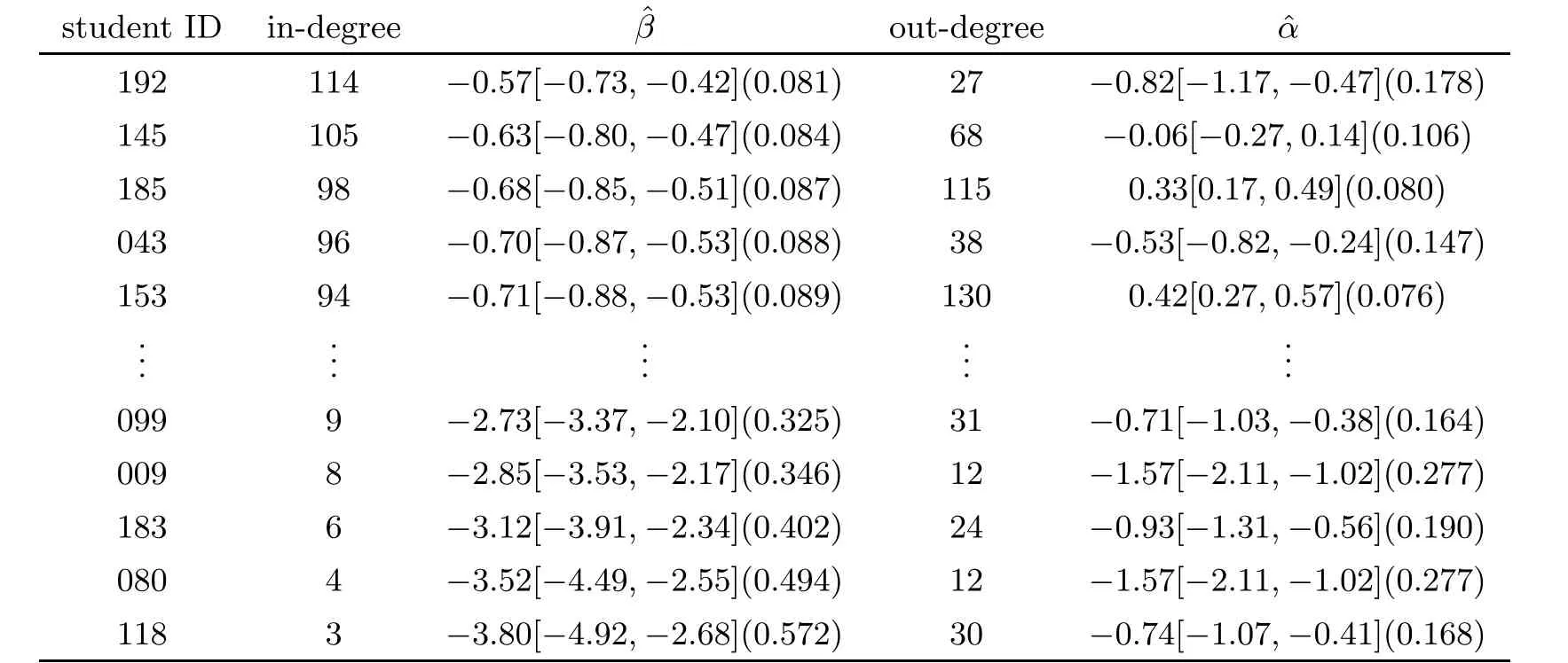
Table 3 The WEBSTER network dataset∗∗

4 Discussions and Future Studies

It is of interest to further study the case that random graphs with the edges taking infinite non-negative integer valued weights by considering Poisson[25]and discrete compound Poisson random variables,seeing[28].It will be a challenge problem that we can extends the weights to unbounded variable.

5 Proof of Theorems

In this section we give proofs for the lemmas and theorems presented in Section 2.

5.1 Preliminaries

We start with some notations.For a vector,denote bythe-norm of x.For an n×n matrixdenote the matrix norm induced by the-norm on vectors in Rn,that is,We introduce a class of matrices.Given two positive numbers m and M with M≥m>0,we say the(2n−1)×(2n−1)matrix V=(vi,j)belongs to the class Ln(m,M)if the followings holds:

where δi,j=1 when i=j and δi,j=0 when

We define another matrix normfor a matrix A=(ai,j)byTo quantify the accuracy of this approximation,[24]prove the following proposition.

Proposition 5.1Ifwiththen for large enough n,

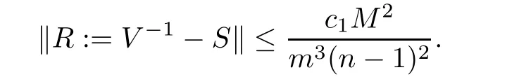
where c1is a constant that does not depend on M,m,and n.

5.2 Proof of Theorem 2.1

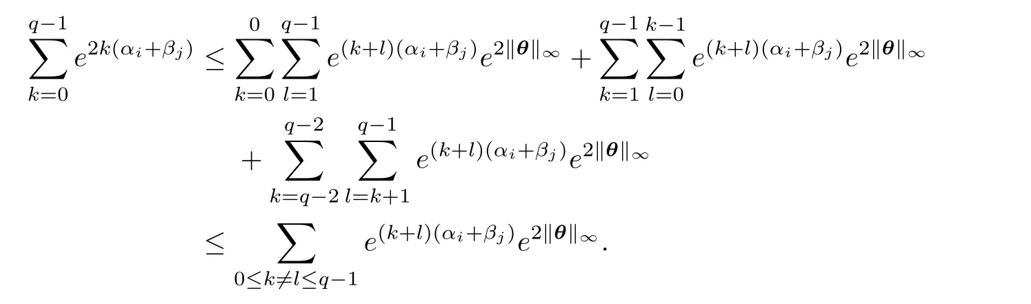
Regarding the asymptotic normality ofwe note that bothandare sums of n−1 independent Bernoulli random variables.By the central limit theorem for the bounded case in Theorem 4.2 of[4],we know thatandare asymptotically standard normal if vi,idiverges.By equation(2.2),we will give vi,is proof.Becausewe have

Therefore,we have

Combining the above three inequalities,it yields that

On the other hand,it is easy to verify that

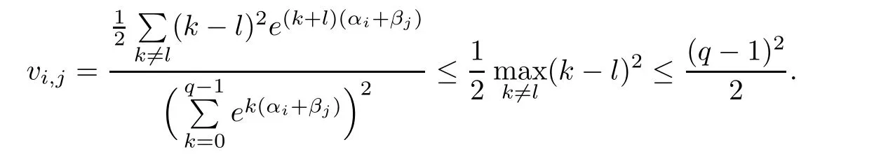
According to the definition of Ln(m,M),we have

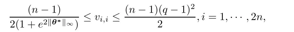
Then,we have

By Theorem 4.2 of[4],we have the following proposition.

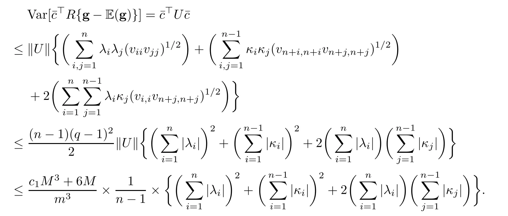
Proposition 5.2Assume thatandas n→∞,thenE(g))is asymptotically normally distributed with mean zero and variance

Before proving Theorem 2.1,we show lemmas below.

Lemma 5.3Let R=V−1−S andThen,

ProofThe proof of Lemma 5.3 is similar to that of Lemma A3 in[24]and we omit it here.

Lemma 5.4LetandAssume thatwhere τ∈(0,1/24)is a constant.LetandThen,

ProofNote that

By Lemma 5.3,we have

Therefore,we have

Consequently,

The following lemma is because of Theorem 1 and Theorem 2 in[27].

Lemma 5.5Assume thatwithwhereis a constant,and thatwhere Pθ∗ denote the probability distribution(2.1)on A under the parameter θ∗.Then,as n goes to infinity,with probability approaching one,the MLEexist and satisfies

Furthermore,if the MLE exists,it is unique.

Lemma 5.6Assume thatwhere τ∈ (0,1/36),then for any fixed k≥1,as n→∞,the vector consisting of the first k elements ofis asymptotically multivariate normal with mean zero and covariance matrix given by the upper left k×k block of S.

Proof of Theorem 2.1By Lemma 5.5,with probability approaching one,we have

The following calculations are based on the event(5.7).Let.By Taylor’s expansion,for anywe have

where

Equivalently,

Note that

and

then we have

It is easy to obtain

We have

and by Proposition 5.1,we have

Therefore,

where c1is given in Proposition 5.1.

Therefore,by Chebyshev’s inequality,

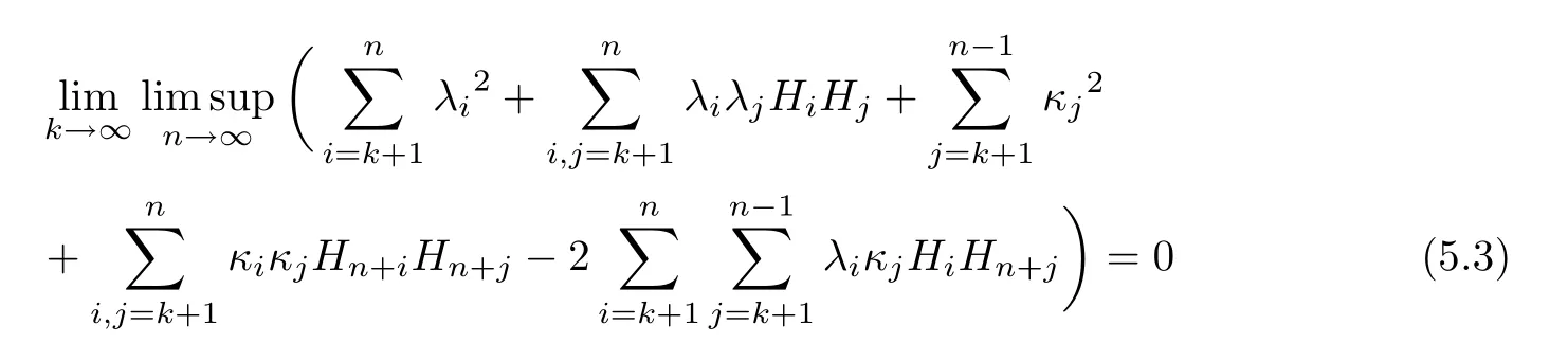
In view of(5.14)and(5.15)and Lemmas 5.4,5.5,and 5.6,if,where 0<τ<1/36 is a constant,and conditions A1 and A2 hold,then

Therefore,Theorem 2.1 immediately comes from Proposition 5.2.