INFINITELY MANY SOLUTIONS WITH PEAKS FOR A FRACTIONAL SYSTEM IN RN∗

2020-06-04 08:49

Acta Mathematica Scientia(English Series) 2020年2期

Department of Mathematics and Information Science,Guangxi Center for Mathematical Research,Guangxi University,Nanning 530003,China

E-mail:heqihan277@163.com

Yanfang PENG(彭艳芳)

School of Mathematics Science,Guizhou Normal University,Guiyang 550001,China

E-mail:pyfang2005@sina.com

Abstract In this article,we consider the following coupled fractional nonlinear Schrödinger system in RN

Key words Fractional system;solutions with peaks;synchronized;segregated

1 Introduction

Here we study the following fractional nonlinear Schrödinger system in RN

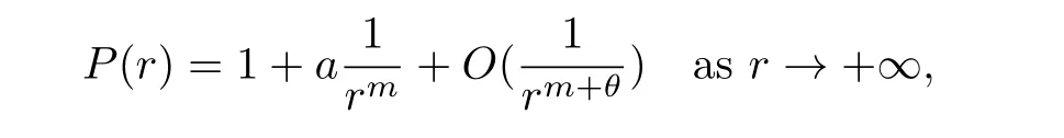
whereP(x)andQ(x)are continuous bounded radial functions,N≥2,00,µ2>0,andβ∈R is a coupling constant,and

where i is the imaginary unit.This fractional Schrödinger system is an important and interesting model in the study of particles on stochastic fields modelled by Lévy processes in fractional quantum mechanics,which was discovered by Laskin[16,17]as a result of expanding the Feynman parth integral from the Brownian-like to the Lévy-like quantum mechanical paths.

Problem(1.1)can be seen as a counterpart of the following fractional equation

On the basis of the minimization on the Nehari manifold,Secchi[26]found ground states for(1.3).Felmer,Quaas,and Tan[11]studied the existence of positive solutions for the fractional nonlinear Schrödinger equation

(P2)There are constantsa∈R,m>1,andθ>0,such that asr→+∞,

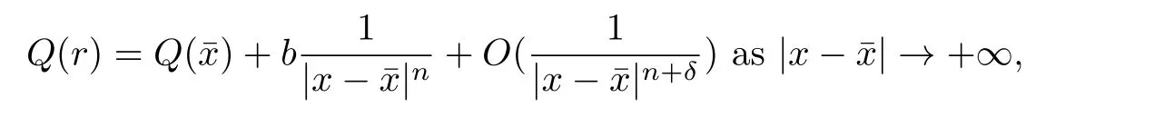
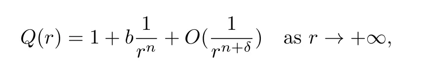
(Q2)There are constantsb∈R,n>1,andδ>0,such that asr→+∞,

whereaandbsatisfy some assumptions.In finitely many non-radial positive segregated solutions were also constructed by Peng and Wang[25]for system(1.1)whenP(x)andQ(x)satisfy the above conditions(P1),(P2),(Q1)and(Q2)andβ<β∗,wherem=n,a>0,b>0,andβ∗is a positive constant.

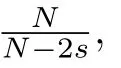
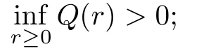
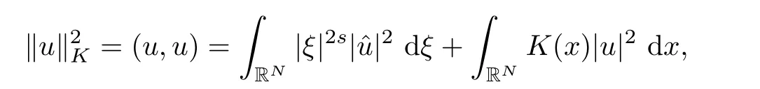
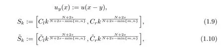
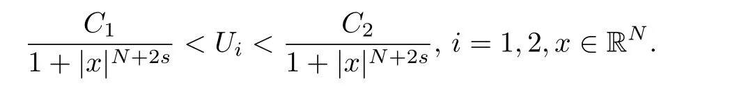
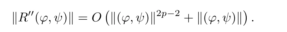
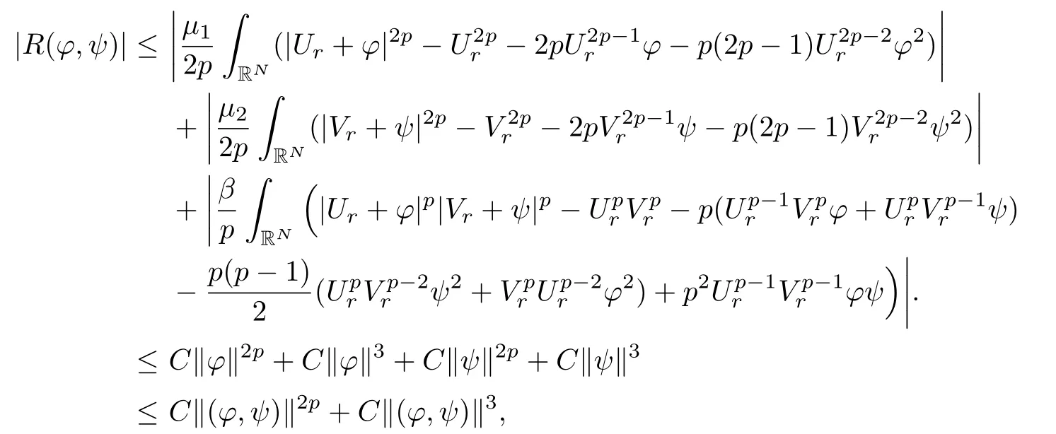
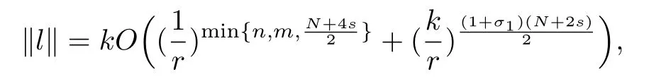
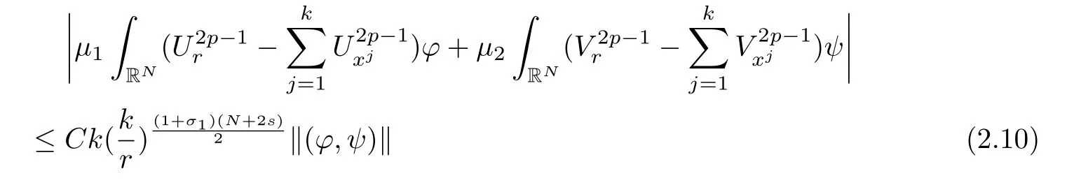
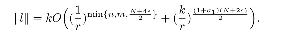
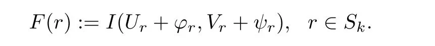
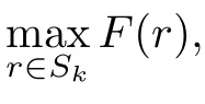
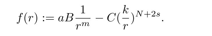
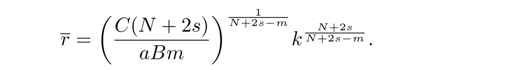
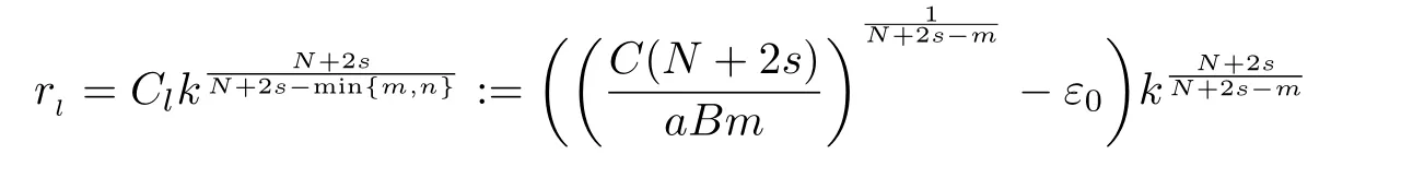
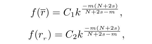
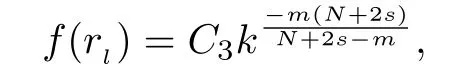
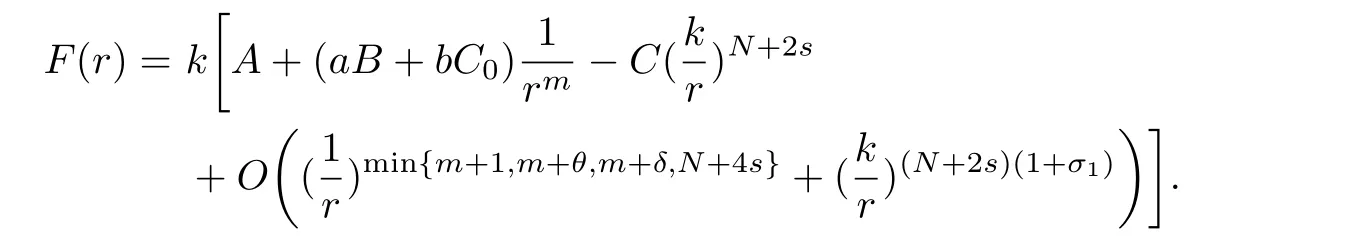
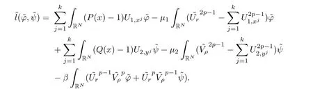
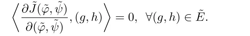
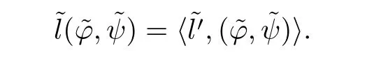
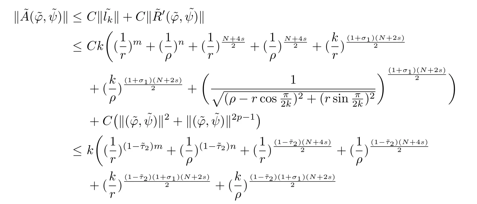
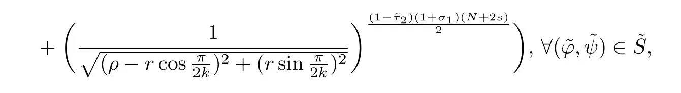
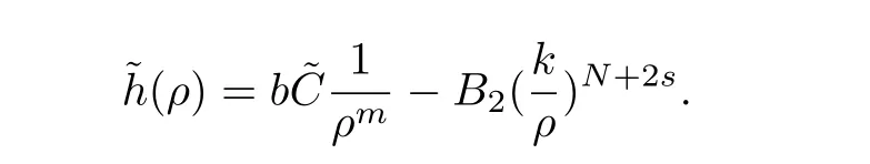
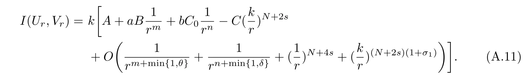
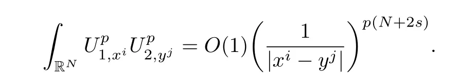
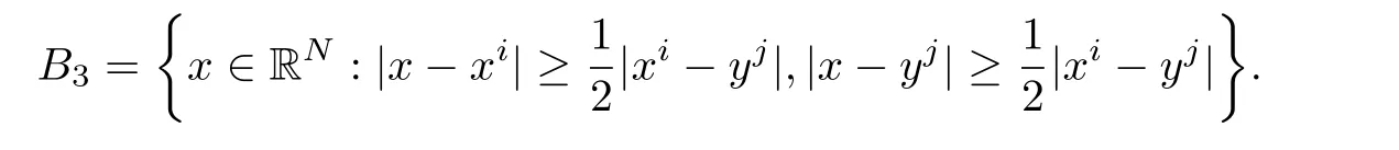
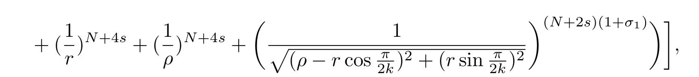
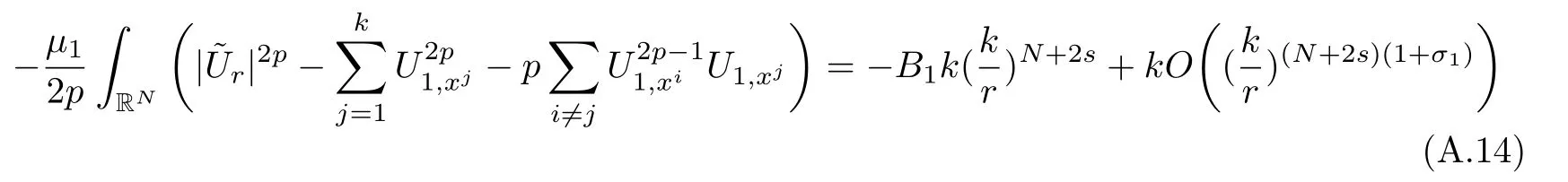
Here we should stress that the results mentioned above are either for the single equation or for system(1.1)withs=1 andp=2.Although there is a wide range of literature studying existence and multiplicity for single equation and system(1.1)withs=1 andp=2,to our knowledge,there are few articles dealing with similar results for fractional system,with the exception of our result[14],where we showed the existence,non-degeneracy of proportional positive solutions and the form of least energy solutions for(1.1)withP(x)=Q(x)≡1 under some assumptions onµ1,µ2,p,andβ.This observation prompts us to study system(1.1).The results of[25]bring us a nature question:whether there are infinitely many non-radial synchronized or segregated vector solutions for system(1.1)with 0

For simplicity,we always assume thatµ1>µ2,and set

where 0<β0<β1are the roots of

and

whereχis a characteristic function andσ1will be defined in Lemma 2.4.

Remark 1.1The conditions(A1)–(A7)are the same as[14],where with(A1)–(A7),the existence and non-degeneracy of proportional positive solutions were ensured.In this article,we also need(A1)–(A7)to obtain the non-degeneracy of proportional positive solutions in Theorem 1.2 or Theorem 1.3.

Our results are as follows:

Theorem 1.2Suppose thatN≥2,0µ2>0,P(x)andQ(x)satisfy(P1),(P2),(Q1)and(Q2),and min{m,n}0 and a decreasing sequencesuch that forandk0

(1)m0 andb∈R;orm>n,a∈R andb>0;

(2)m=n,aB+bC0>0,whereBandC0are defined in Proposition A1.Furthermore,

whereτ0will be given in(1.13).

Theorem 1.3Suppose that1,1µ2>0,P(x)andQ(x)satisfy(P1),(P2),(Q1)and(Q2),min{m,n}

(1)m0 andb∈R;orm>n,a∈R andb>0;

(2)m=n,aB+bC0>0,whereBandC0are defined in Proposition A1.Furthermore,

whereAi(i=1,2,···,7)are given in(1.5)andτ0will be given in(1.13).

Theorem 1.4Suppose thatN=2 or 3,00,P(x)andQ(x)satisfy(P1),(P2),(Q1)and(Q2),a>0,b>0 andm=n0 andk0>0 such that forβ<β0andk0

Before we close the introduction,we introduce some notations to be used in the proofs of our main results and formulate a version of the main results which give more precise descriptions about the non-radial synchronized and non-radial segregated character of the solutions.In doing so,we also outline the main idea and the approach in the proofs of Theorems 1.2,1.3,and 1.4.

Define

whereHs(RN)is the usual fractional Sobolev space with the norm for any bounded measurable functionK(x)

and defineH:=Hs×Hsendowed with the following norm

Set

whereandwill be determined later,and

According to the result of[13],the following equation

has a radial regular non-degenerate positive solutionw,which satisfies

with some constantsC2>C1>0.Moreover,in[14],with the assumptions of Theorem 1.2 or Theorem 1.3,we have proved that there exists a radial non-degenerate positive solution of the form

for the following system:

whereτ0andk1are two positive constants,dependent ofp,µ1,µ2,andβ.

We set

We will verify Theorem 1.2 and Theorem 1.3 by proving the following result.

Theorem 1.5Under the assumptions of Theorem 1.2 or Theorem 1.3,there exists a constantk0>0,such that for anyk0

where(φ(x),ψ(x))∈Hand

for some small constantσ>0.

LetUi(i=1,2)be the radial regular non-degenerate positive solution of the following problem

According to the result of[13],it holds that there exist two constantsC2>C1>0 such that

In this article,we will use(U1,U2)to build up the approximate solutions for(1.1).

Denote

where

Let

wherexjis defined in(1.11).

To prove Theorem 1.4 is equivalent to showing the following result:

Theorem 1.6Under the assumptions of Theorem 1.4,there existk0>0 andβ0>0 such that whenβ<β0and for anyk0

for some small constantσ>0.

Remark 1.7Radial symmetry can be replaced by the following weaker symmetry assumption:after suitably rotating the coordinate system,

(P′)P(x)=P(x′,x3,···,xN)=andP(x)has the following expansion:where∈RN,a∈R,m>1,θ>0 andP()>0 are constants.

(Q′)Q(x)=Q(x′,x3,···,xN)=andQ(x)has the following expansion:

This article is organized as follows.In Section 2,we will study the finite-dimensional reduced problem and prove Theorem 1.5.We will put the study of the existence of segregated solutions for system(1.1)and the proof of Theorem 1.6 into Section 3.We will give all the technical calculations in Appendix A.

2 Synchronized Vector Solutions and the Proof of Theorems 1.2 and 1.3

In this section,we consider synchronized vector solutions and prove Theorem 1.2 and Theorem 1.3 by proving Theorem 1.5.We define the functional corresponding to(1.1)by

Then it is easy to see thatI∈C1(H)and its critical points correspond to the solutions of(1.1).

Define

wherexjis defined in(1.11)and set

Let

Becauseτ0Ur=Vr>0 fork∈N+andx∈RN,we can expandJ(φ,ψ)as follows:

where

and

To find a critical point(φ,ψ)∈EforJ(φ,ψ),we need to discuss each term in the expansion(2.4).

It is easy to check that

is a bounded bi-linear functional inE.Thus there exists a bounded linear operatorL:E→Esuch that

In view of the above analysis,we have the following result.

Lemma 2.1There is a constantC>0,independent ofk,such that for anyr∈Sk,

Next,we discuss the invertibility ofL.

Lemma 2.2There exist two constantsC0>0 andk0>0,such that fork0

ProofThe proof of the Lemma is similar to that of Lemma 2.2 in[25].So,we omit it.

Lemma 2.3For any(φ,ψ)∈E,we have

and

ProofBy direct calculation,for any(u1,v1),(u2,v2)∈E,we have

where we have used the fact that for anyt1,t2∈R,p>1,

Similarly,we have

and

So,we complete the proof.

Lemma 2.4There exists a small constantσ1∈(0,σ)such that

whereσis defined in(1.6).

Proof

and there exists a constantσ1∈(0,σ)such that

and

Combining(2.9),(2.10),(2.11)and the definition ofl,we can deduce that

Moreover,there exists a constantC>0 such that

ProofIt follows from Lemma 2.4 thatlis a bounded linear functional inE.Thus,there exists anl′∈Esuch thatThus, finding a critical point forJ(φ,ψ)is equivalent to solving

By Lemma 2.2,Lis invertible.Hence,(2.12)can be written as

We choose a small constant 0<τ2<τ,whereτis defined in(1.7),and set

Forksufficiently large,

which implies thatAis a mapping fromStoS.

On the other hand,forksufficiently large,

Then,we see that whenkis sufficiently large,Ais a contraction mapping fromStoS.By the contraction mapping theorem,we completes the proof.

Now,we are ready to prove Theorem 1.5.Letbe the mapping obtained in Proposition 2.5.Define

With the same argument as in[15]or[18],we can easily check that ifris a critical point ofF(r),then(Ur+φr,Vr+ψr)is a critical point ofI.

Proof of Theorem 1.5It follows from Lemmas 2.1 and 2.3 that

Then,following from Lemma 2.4 and Proposition A2,we have

Without loss of generality,we may also assume thatn>m.So,

whereA,B,andCare fixed positive constants.

Let

By the assumptions of Theorems 1.2 and 1.3,we know thata>0.Then by direct calculation,we know thatf(r)has a local maximum point

Set

and

Then,we can find a constantε0>0 such that

and

where 0

By direct calculation,we can choose a constantsuch that whenkis sufficiently large,

On the other hand,

Hence,F(r)has a local maximum pointrkinSk,andrkis an interior point ofSk.Thus,rkis a critical point ofF(r).As a result,(Urk+φrk,Vrk+ψrk)is a solution of(1.1).

For the casem>n,we can obtain our results with the same method.

For the casem=n,then

Let

Using the above methods,we can prove the results.So far,we complete our proof.

3 Segregated Vector Solutions and the Proof of Theorem 1.4

In this section,we consider segregated vector solutions and prove Theorem 1.4 by proving Theorem 1.6.Let

wherexjandyjare defined in(1.11)and(1.16),respectively.

We assume that

Define

Let

From the above analysis,we have the following lemma.

Lemma 3.1There exists a constantC>0,independent ofk,such that for any(r,ρ)

Lemma 3.2There existk0>0,β0>0,andC0>0,such that forβ<β0and anyk>k0andwe have

ProofThe proof is similar to that of Lemma 3.2 in[25]and we omit it.

From(2.9),(2.10),and Lemma A3,we can obtain the following Lemma.

Lemma 3.3There exists a small constantσ1such that

whereσ1is defined in Lemma 2.4.

Proposition 3.4Forksufficiently large,there exists aC1-mappingwithsatisfyingand

Moreover,there exists a constantC>0 such that

ProofFrom the definition ofwe know thatis a bounded linear functional in.Thus,it follows from Reisz Representation Theorem that there is ansuch that

So, finding a critical point ofis equivalent to solving

Forksufficiently large,

On the other hand,forksufficiently large,

Thus,whenkis sufficiently large,is a contraction mapping fromtoSo,our results follow from the contraction mapping theorem.This completes the proof.

Now,we are ready to prove Theorem 1.6.Letbe the mapping obtained in Proposition 3.4.Define

We can check that forksufficiently large,if(r,ρ)is a critical point ofthenis a critical point ofI.

Proof of Theorem 1.6From Lemmas 2.3 and 3.3,and Proposition A5,we have

Now,we will consider the maximization problem:

In the following,we claim that(r1,ρ1)is an interior point of

Denote

and

By direct calculation,we see thatandattain the local maximum at

and

respectively.So,we can find a small constantε0>0 such that if we set

and

then

and

whereC1,C2,C3,d1,d2,andd3are constants satisfying 0

and

From(3.5)–(3.9),we can see that whenkis sufficiently large,the local maximization ofcan not be obtained at the boundary of.That is,(r1,ρ1)is an interior point ofThus,(r1,ρ1)is a critical point ofwhich means thatis a solution of(1.1).This completes the proof.

Appendix

A1 Energy estimate

In this section,we will give out some energy estimates of the approximate solutions.Recall that