INFINITE SERIES FORMULAE RELATED TO GAUSS AND BAILEY-SUMS∗

Wenchang CHU

School of Mathematics and Statistics,Zhoukou Normal University,Zhoukou 466001,China

Department of Mathematics and Physics,University of Salento(P.O.Box 193),73100 Lecce,Italy

E-mail:chu.wenchang@unisalento.it

Abstract The unified Ω-series of the Gauss and Bailey-sums will be investigated by utilizing asymptotic methods and the modified Abel lemma on summation by parts.Several remarkable transformation theorems for the Ω-series will be proved whose particular cases turn out to be strange evaluations of nonterminating hypergeometric series and infinite series identities of Ramanujan–type,including a couple of beautiful expressions for π and the Catalan constant discovered by Guillera(2008).

Key words Abel’s lemma on summation by parts;classical hypergeometric series;Gauss’-sum;Bailey’s-sum;Saddle point method;Catalan’s constant

1 Introduction and Motivation

For an arbitrary complex sequence{τk},define the backward and forward difference operators ∇ and,respectively,by

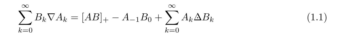
provided that the following limitexists and one of both series is convergent.Recently,this lemma has been successfully utilized in[2,3]to review summation formulae for both classical and basic hypergeometric series.

According to Bailey[4],the classical hypergeometric series reads as

where the rising shifted factorial is given by(x)0≡1 and

with the Γ-function being defined by Euler integral

The multi–parameter forms of the shifted factorials and the Γ-function will be abbreviated,respectively,as

For the nonterminating series in variable“1/2”,there are two well-known formulae due to Gauss and Bailey(Bailey[4,§2.4]),which can be reproduced as

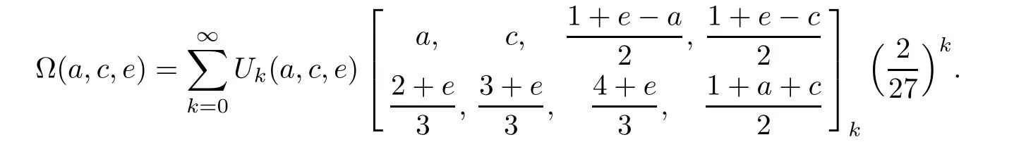
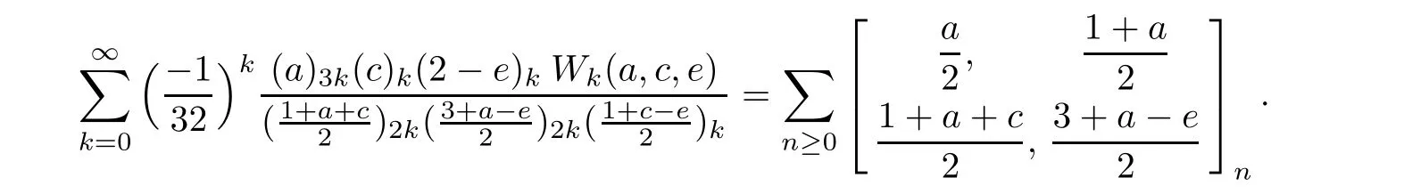
They can be unified to the following Ω-sum

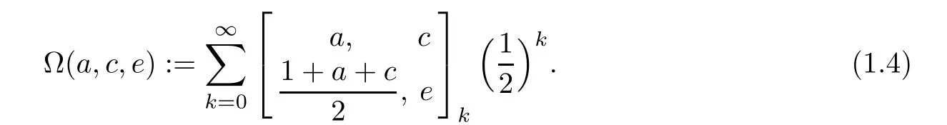
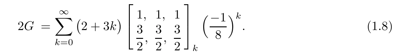
The objective of this article is to investigate the above sum by utilizing asymptotic methods and the modified Abel lemma on summation by parts,which will express the infinite series Ω(a,c,e)in terms of Ω(a+m λ,c+m µ,e+m ν)with the parameters being shifted by m-times of the “recurrence pattern” [λµν].The next section will be devoted to the recurrence pattern[200]and proving an interesting reciprocal relation of Ω(a,c,e).By considering the recurrence pattern[113],we shall establish,in Section 3,four formulae for hypergeometric-series and the following infinite series identities of Ramanujan–type(see Example 3.5):

Then in Section 4,the recurrence pattern [11-1]will be carefully examined that will lead us not only to find two general transformation theorems about Ω(a,c,e),but also to recover the following couple of beautiful expressions for π and the Catalan constant due to Guillera[5,6]:

By making use of the recurrence pattern[311],we shall derive,in Section 5, five transformation formulae for Ω(a,c,e)and seven strange evaluations of nonterminating hypergeometricseries.In the sixth section,the recurrence pattern[31-1]will be employed to extend,with three free parameters,two important transformation theorems of Guillera[6,§2.5]and to evaluate four infinite series with their argument equal toincluding two due to Guillera[6].Finally in Section 7,this article will end with limiting relations and numerous infinite series identities involving π,Catalan’s constant,and harmonic numbers.

Throughout this article,the following useful properties of the Γ-function will be appealed frequently without explanation(Rainville[7,Chapter 2]):

•Recurrence relation

•Asymptotic relation

•Euler reflection formula

•Gauss multiplication formula

2 Recurrence Pattern[200]

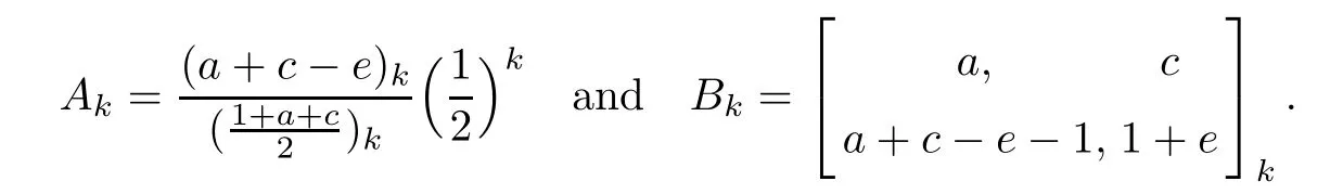
For the two sequences Akand Bkgiven respectively by

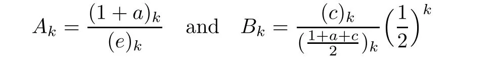
it is not difficult to check the differences

as well as two limiting relations

Then,by means of the modified Abel lemma on summation by parts,we can manipulate the Ω-series as follows:

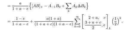
which can be equivalently stated as the following recurrence relation:

Iterating m-times this equation,we get the partial sum expression.

Lemma 2.1(Recurrence pattern[200])

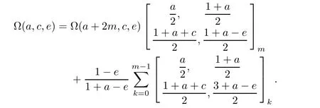
Its limiting case m→∞results in the following interesting transformation.

Theorem 2.2(Transformation formula:ℜ(1+c−e)>0)

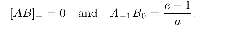
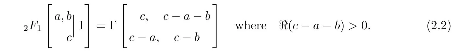
This theorem may serve as a common generalization of both(1.2)and(1.3),as one can easily check that when e=1,it reduces to the former,while a+c=1,to the latter,just evaluating the2F1-series on the right by the first Gauss summation theorem(Bailey[4,§1.3]):

Observe that the sum with respect to k appearing in Theorem 2.2 is invariant under c→ 2−e and e→2−c.By combining the equality in Theorem 2.2 with its reformulation under the aforementioned parameter replacements and then canceling the common sum with respect to k,we can express the resulting equation as

Simplifying further the last expression in the braces to

we find the following interesting formula,where the restriction ℜ(1+c− e)>0 imposed in Theorem 2.2 is removed by analytical continuation.

Corollary 2.3(Reciprocal relation)

We point out that this formula is another common extension of both-series identities(1.2)and(1.3)due to Gauss and Bailey,respectively,that can be verified easily by letting e=1 and a+c=1.

Proof of Theorem 2.2It is obvious that the series displayed on the right is convergent under the condition ℜ(1+c−e)>0.According to(1.10)and(1.12),we also have,as m→∞,

Now that the limiting procedure from Lemma 2.1 to Theorem 2.2 depends only on

it suffices to show the following relation

For each natural number n,we prove first that the last relation holds for e=n+1.Then,(2.3)will follow directly by applying the Carlson theorem(Bailey[4,§5.3]).

By replacing the summation index k by j− n,we can reformulate the Ω-series

It is not difficult to check that for each fixed n∈N,the last expression(2.5)is bounded and can be ignored in comparison withFor the penultimate expression(2.4),evaluating the2F1-series by(1.2)and then applying(1.10)and(1.12),we can estimate it as follows:

In conclusion,we confirm(2.3)when e=n+1 for each fixed n∈N.

3 Recurrence Pattern[113]

Define the sequences Akand Bk,respectively,by

We can easily prove the differences

as well as two limiting relations

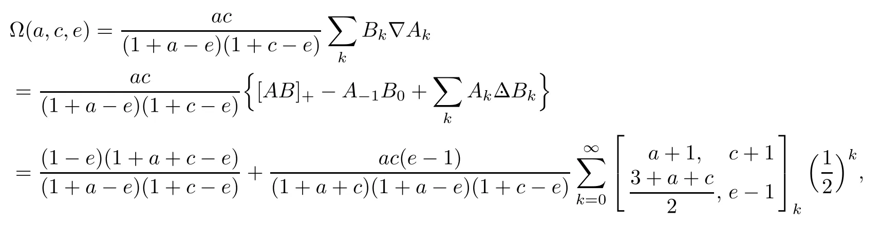
In view of the modified Abel lemma on summation by parts,we can reformulate the Ω-series as

which reads as the following recurrence relation

Writing further Ω(a,c,e+2),by putting the initial term aside,as

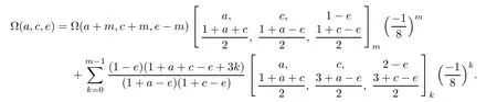
and then substituting this relation into(3.1),we establish,after some simplifications,the following recurrence relation

Iterating this relation m-times and introducing the quadratic polynomial in k

we derive the following partial sum expression.

Lemma 3.1(Recurrence pattern[113])

By appealing to the Weierstrass M-test(Stromberg[8,§3.106])on uniformly convergent series,we derive,from the limiting case m→∞of the last equation,the following transformation.

Theorem 3.2(Transformation formula)

Observing the linear factorizations

we deduce the simplified transformations from the last theorem.

Proposition 3.3(Reduction formulae)

By specifying the parameters a and c such that the Ω-series can be evaluated by(1.2)and(1.3),we get,from the last proposition,the following nonterminating hypergeometric series identities.

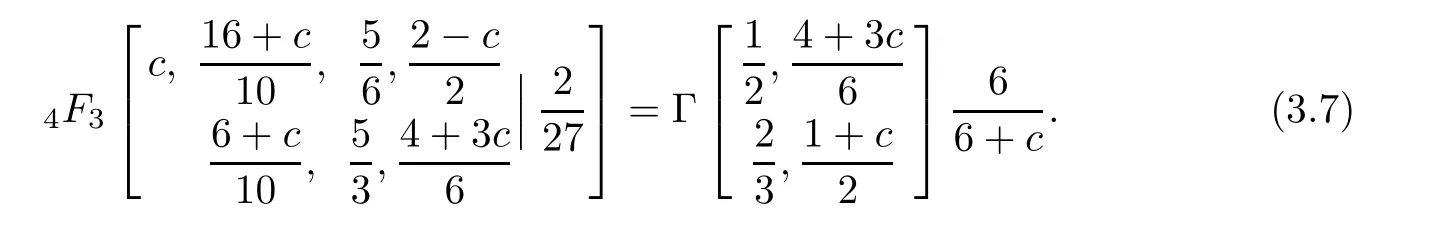
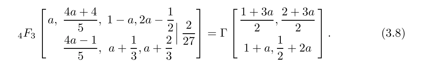
Corollary 3.4(Four closed formulae for hypergeometric series)

•c=1−a in(3.4):

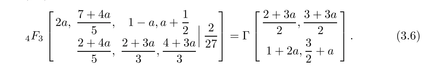
•a=1/3 in(3.4)(Gessel[9,Equation 30.7]for its terminating form):

•c=1−a in(3.5):

•a=2/3 in(3.5)(cf.Gessel[9,Equation 30.4]for its terminating form):

Similar formulae with the same hypergeometric argument“2/27” can be obtained from the limiting cases n→∞of Chu[10,Equations 5.3e-f-g].

Furthermore,we have the following infinite series identities of Ramanujan–type.

Example 3.5(Three infinite series identities)

The last two identities can be considered as counterparts of the following beautiful one due to Ramanujan[11,Equation 31]:

ProofThe first two formulae follow directly by putting a=1/2 in(3.6)and(3.8),where the former(3.10)is discovered by Zhang[12,Example 9].The last series is obtained by letting a=c=1 in(3.5)and then evaluated through(1.2)as follows:

4 Recurrence Pattern[11-1]

Let Akand Bkbe the two sequences defined,respectively,by

We have no difficulty to show the differences:

as well as two limiting relations

According to the modified Abel lemma on summation by parts,the Ω-series can be reformulated as

which yields the recurrence relation below

Iterating m-times this equation and then simplifying the result,we get the following transformation formula.

Lemma 4.1(Recurrence pattern[11-1])

According to(1.10),we have,as m→∞,the following asymptotic relation

It will be quite a challenging task to determine asymptotically the behavior of Ω(a+m,c+m,e−m)as m→∞.We shall tackle this problem by following the procedure described in[13].For the hypergeometric term appearing in Ω(a+m,c+m,e− m)

consider the term ratio

which can be estimated,for k=mε,as follows

Splitting the series Ω(a+m,c+m,e− m)into four parts,we can write it explicitly

We are going to show that among the four sums just displayed,the first one is dominant,while the other three sums are negligible.

4.1 The three negligible sums

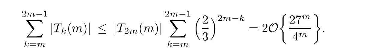
By means of(1.10)and(1.12),we can approximate the following three terms:

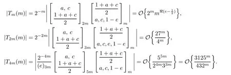
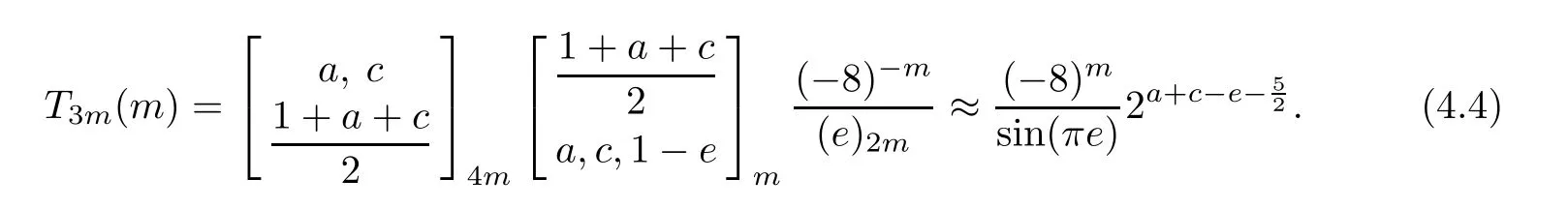
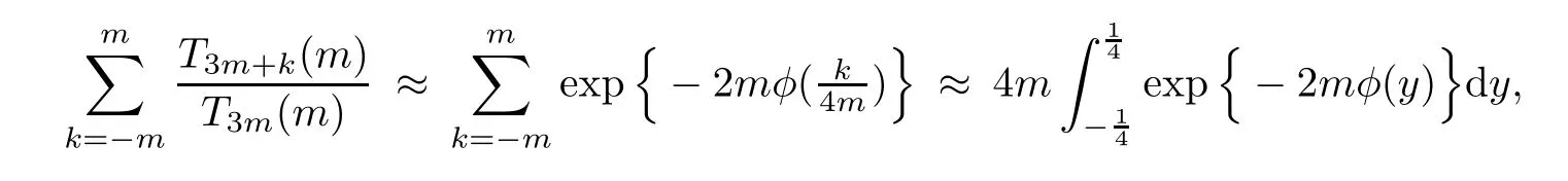
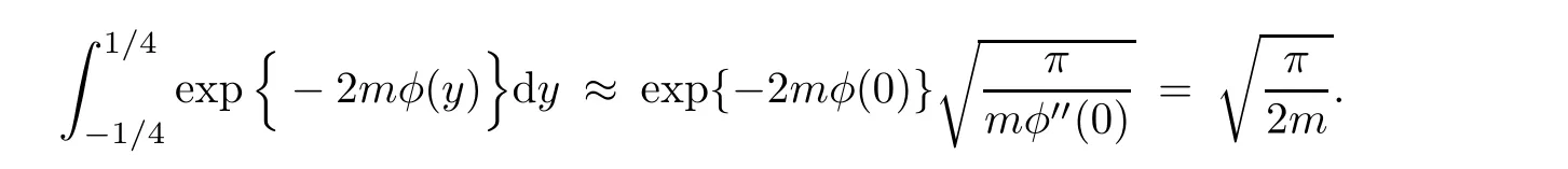
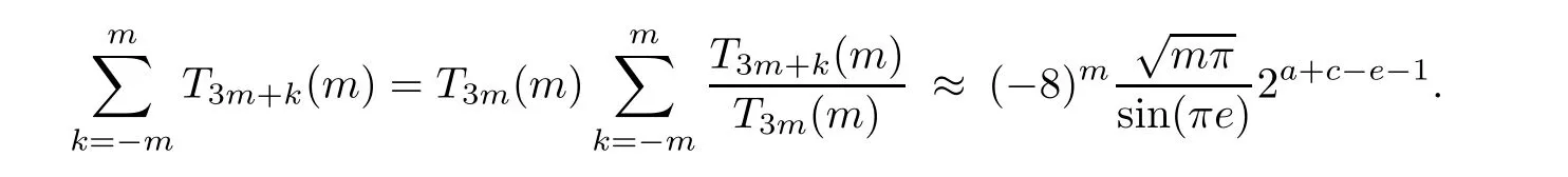
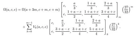
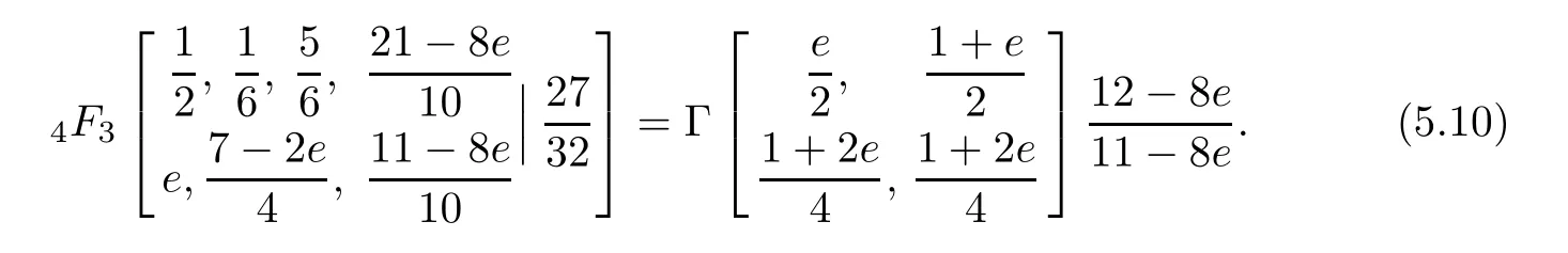
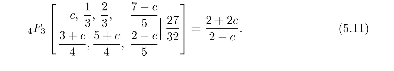
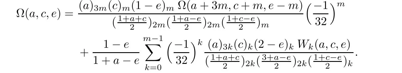
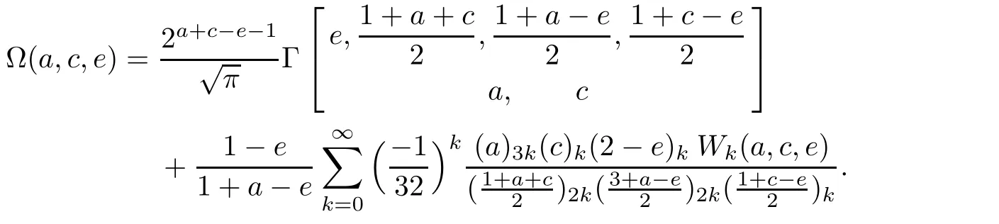
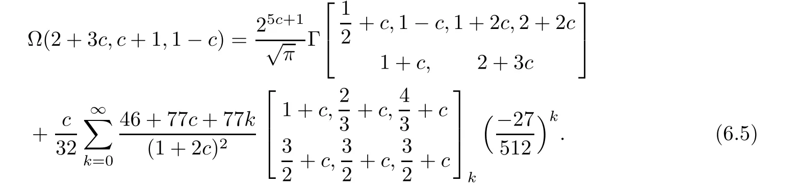
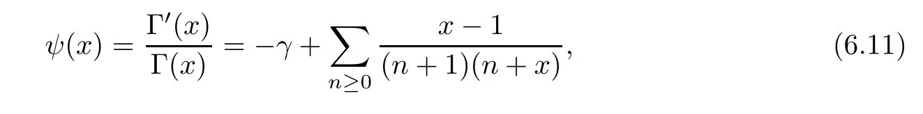
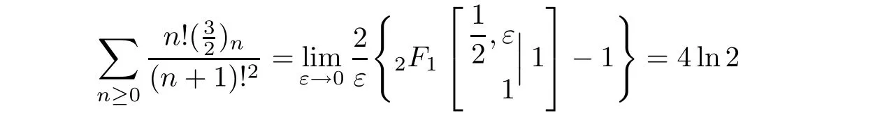
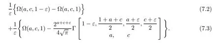
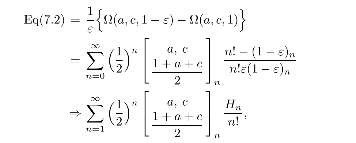
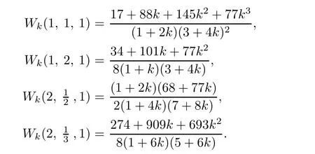
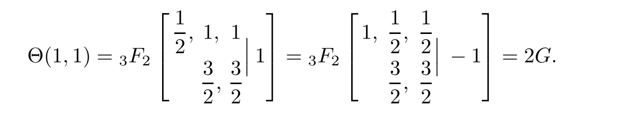
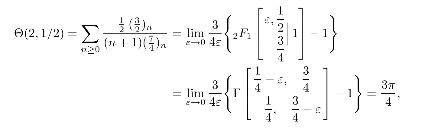
First,for 0≤k

Finally,for 4m

For the last three truncated sums,it is routine to verify that when m→∞,they are annihilated by the factor displayed in(4.2).Therefore,they can be ignored from the limiting expression.

4.2 The dominant sum

It remains to estimate the truncated sum with respect to k over 2m≤k<4m.According to the previously displayed term ratio(4.3),Tk(m)is almost unimodal with the maximum equal to T3m(m).

By combining(1.10),(1.11),and(1.12),we can evaluate the following limit as m→∞

Now,we have to estimate the remaining truncated sum

For an indeterminate x independent of k and m with 0≤k≤m,it is not hard to check the following two asymptotic relations:

Then,the general hypergeometric term ratio can be estimated as

This leads us to the following integral expression

where the function φ(y)is defined by

with the first two derivatives being given by

Therefore,y=0 is the global minimum of φ(y)for y>The saddle point method(also called the steepest descent method,cf.[14,§5.7])asserts that

Combining this result with(4.4),we find the following asymptotic relation

4.3 Transformation formulae

Letting m→∞in Lemma 4.1 and then taking into account of(4.2)as well as the four estimations of the truncated sums,after the replacement e→2−e and slight simplifications,we establish the following transformation.

Theorem 4.2(Transformation formula)

This theorem may be considered as a three–parameter extension of Guillera’s important result[6,Equation 6],which can be obtained by lettingin this theorem.Furthermore,letting a=c=e=1/2 in Theorem 4.2,we recover the following beautiful π-series expression.

Example 4.3(Guillera[6,§2.3])

Performing the replacement e→2−e in Theorem 2.2 and then substituting the resulting expression into Theorem 4.2,we get another transformation formula.

Theorem 4.4(Transformation formula:ℜ(c+e)>1)

In this theorem,letting a=c=e=+x,we recover another formula due to Guillera[6,Equation 5].Alternatively,letting e=1−a in Theorem 4.4 and then evaluating the series on the right by(2.2),we find the following remarkable summation formula for the quadratic series.

Corollary 4.5(Quadratic series formula)

5 Recurrence Pattern[311]

By picking out the first term,rewrite Ω(a+2,c,e)as

Substituting this relation into(2.1)and then simplifying the resulting equation,we get the following recurrence relation:

Iterating this relation m-times and defining the quadratic polynomial in k

we get the following partial sum expression.

Lemma 5.1(Recurrence pattern[311])

Letting m→∞in the last equality results directly in the transformation below.

Theorem 5.2(Transformation formula)

According to the decompositions into linear factors

we deduce from the last theorem the following simplified transformations.

Proposition 5.3(Four reduction formulae)

In this proposition,by specifying the parameters a,c,e such that the corresponding Ω-series can be evaluated by(1.2)and(1.3),we derive the following nonterminating hypergeometric series identities.

Corollary 5.4(Seven closed formulae for hypergeometric series)

•a=2c in(5.3):

•c=1−a in(5.3):

•e=1 in(5.4):

•c=1/2 in(5.4):

•e=1 in(5.5)(cf.Gessel[9,Equation 30.8]for its terminating form):

•c=4−3e in(5.5):

•c=5−3e in(5.6):

By specifying parameters in these formulae,it is possible to derive further identities of particular interest.For example,letting e=3/2 in(5.10)results in the following strange zero sum that the author is unable to prove it directly:

6 Recurrence Pattern[31-1]

For the Ω-sum defined in(1.4),applying first(2.1)and then(4.1),we have the following recurrence relation

Iterating this relation m-times and then introducing the rational function

we obtain the following equality.

Lemma 6.1(Recurrence pattern[31-1])

Theorem 6.2(Transformation formula)

There are many different decompositions of Wk(a,c,e)into linear factors for particular choices of a,c,and e.By examining two typical expressions

we get from the last theorem the following simplified transformations.

Proposition 6.3(Two reduction formulae)

It should be pointed out that the first formula displayed in the last proposition is equivalent to Guillera[6,Equation 10]under the replacement c→x−.Letting c→−1/2 in(6.5)and(6.6)and then simplifying the results,we get the following two formulae,where the first has been discovered by Guillera[6,§2.5].

Example 6.4(Two infinite series identities)

Furthermore,by combining Theorem 6.2 with Theorem 2.2,we get the following transformation formula,which extends another important formula due to Guillera[6,Equation 9]with three free parameters.

Theorem 6.5(Transformation formula:ℜ(1+c−e)>0)

In view of(6.3)and(6.4),this theorem contains the following particular cases.

Corollary 6.6(Two reduction formulae)

Recall the digamma function(Rainville[7,§9])

where γ is the Euler–Mascheroni constant.It is not hard to deduce the following approximation

Specifying c=0 and c=2,respectively,in(6.9)and(6.10),and then making use of the two relations

we can evaluate the infinite series

and

which lead us to the interesting summation formulae below.

Example 6.7(Two infinite series identities)

7 Limiting Relations

Observe that there is a common expression

appearing in Theorems 2.2,4.2 and 6.2.This is quite an interesting phenomenon.Replacing e by 1− ε in this expression and then dividing it by ε,we are going to determine its limit e → 1.

For the sake of brevity,define the function λ(a,c)by

Lemma 7.1(Limiting relation)

ProofThe expression in the first line can be split into two terms

When ε→ 0,the limit of(7.2)can be determined directly as follows:

where we have utilized the approximation(6.12).Putting the last two expressions for(7.2)and(7.3)together,we confirm the limiting relation in Lemma 7.1. ?

According to Lemma 7.1,the limiting relations of Theorems 2.2,4.2 and 6.2 as e→1 are determined by the following theorem.

Theorem 7.2For ℜ(c)>0,let Θ(a,c)be the bivariate function defined by

Then,Θ(a,c)is symmetric and has the following expressions:

Observing the following alternative expression

it is routine to check,with Mathematica commands,the following special values:

Under the same parameter settings,we have also the following factorizations:

They will be employed,in the sequel,to derive several infinite series identities involving π,Catalan’s constant,and harmonic numbers.

Example 7.3(a=c=1 in Theorem 7.2)

The second identity is due to Guillera[6,§2.3]that may be considered as a counterpart of Example 4.3.Different proofs can be found in Lima[15]and Chu–Zhang[1,Example 88].Two other identities may have appeared in the vast literature on Catalan’s constant,even though the author fails to locate them in[16–18]and Finch[19,§1.7].

ProofRecall the well–known Catalan constant

According to Whipple’s quadratic transformation[20,1927]

we derive another expression(Bradley[17,Equation 61]and Lima[15])

Now,letting a=c=1 in Theorem 7.2 and then simplifying the result,we get the desired infinite series identities. ?

Instead,letting a=1 and c=2 in Theorem 7.2 and then evaluating

we can deduce the following three identities,where the first one is well-known that can also be verified by series rearrangements.

Example 7.4(a=1 and c=2 in Theorem 7.2)

Alternatively,letting a=2 and c=1/2 in Theorem 7.2 and then evaluating

we obtain the following infinite series identities.

Example 7.5(a=2 and c=1/2 in Theorem 7.2)

Finally,letting a=2 and c=1/3 in Theorem 7.2 and then evaluating

we establish the following infinite series identities.

Example 7.6(a=2 and c=1/3 in Theorem 7.2)

Concluding commentsBeside those displayed in this article,there exist many other recurrence relations for the Ω-sum.From them,one may expect to derive new infinite series identities of Ramanujan-type as well as summation and transformation formulae for nonterminating hypergeometric series.The interested reader is encouraged to make further attempts.