Aerodynamic/aeroacoustic variable-fidelity optimization of helicopter rotor based on hierarchical Kriging model

Yuepeng BU, Wenping SONG, Zhonghua HAN, Yu ZHANG, Liang ZHANG

School of Aeronautics, Northwestern Polytechnical University, Xi’an 710072, China

KEYWORDS Aeroacoustics;Design optimization;FW-Hpds equation;Helicopter rotor;RANS equations

Abstract Rotor noise is one of the most important reasons for restricting helicopter development;hence, the optimization design of rotor blade considering aeroacoustic and aerodynamic performance at the same time has always been the focus of research attention. For complex rotor design problems with a large number of design variables, the efficiency of the traditional Kriging model needs to be improved. Thus, Hierarchical Kriging (HK) model is employed in this study for rotor optimization design. By using the validated RANS solver and acoustic method based on the FWHpds equation, an efficient aerodynamic/aeroacoustic optimization method for high-dimensional problem of rotors in hover based on HK model is developed. By using present HK model and new infill-sampling criteria, the number of design variables is increased from less than 20-53.Results of two analytical function test cases show that the HK model is efficient and accurate in calculation. Subsequently, the helicopter rotor blade is optimally designed for aerodynamic/aeroacoustic performance in hover based on the HK model with high dimensional design variables. The objective function is adopted to improve the rotational noise characteristics by reducing the absolute peak of the acoustic pressure. In addition, the constraints of thrust, hover efficiency, solidity,and airfoils thickness are strictly satisfied. Optimization results show that the Kriging model finds the objective of reducing the noise by 2.87 dB after 248 iterations while the HK model does it only after 164 iterations.The optimization efficiency of the HK model is significantly higher than that of the traditional Kriging model. In the case analyzed, the HK model saves 35% of the time used by the Kriging model.

1. Introduction

Helicopters have the unique vertical take-off and landing abilities and flexible low-speed maneuverability, hence, they play an irreplaceable role in military and civilian operations. However,they often generate strong noise during horizontal flights and landing maneuvers,causing serious noise pollution.Rotor noise has always been an important factor restricting the development of helicopters. Therefore, more and more institutions,experts and scholars have carried out relevant research on optimization design of noise reduction for helicopter rotors.Due to the complexity of the rotor aerodynamics, there are some challenging problems of rotor optimization design, such as the optimization efficiency for high dimensional problems.The purpose of this study is to improve the rotor blade optimization efficiency for high dimensional problems.

The following part reviews the literature from four aspects:optimization methods,rotor flowfield simulation,acoustic prediction methods, and rotor optimization design.

Commonly used optimization algorithms can be mainly divided into three types:(A) Heuristic algorithm, such as Genetic Algorithms1(GA), Simulated Annealing algorithm(SA), etc.They are global optimization methods, but an enormous amount of calculations are required.(B)Gradient-based optimization algorithm, with the gradients evaluated by adjoint method, which is very efficient, but can be easily trapped into local optimum.(C)Surrogate-based optimization algorithm, such as Efficient Global Optimization (EGO),2which has been proven that it can remarkably improve the efficiency of optimization3-6and has the capability of finding global optima, but it shows low efficiency for high-dimensional optimization problems. Therefore, this study aims at improving the efficiency of surrogate-based optimization in solving high-dimensional problems based on a Hierarchical Kriging(HK)model. Common surrogate models include polynomial Response Surfaces Model(RSM),7,8Kriging models,2,9Radial Basis Functions (RBFs),10Neural Networks (NN),11,12, etc.Among them, the Kriging model is one of the most representative methods. It was first proposed by the South African geologist Krige2in 1951, and later developed and improved by the French mathematician Matheron.9On the basis of the Kriging model, the Cokriging model, an more efficient and predictable variable-fidelity model, was proposed by Kennedy and O’Hagan in 2000.13It has been applied to numerical simulation experiments in the engineering field.Han et al.14implified the calculation of the correlation function of the Cokriging model, optimizing the model hyper-parameter is more than that of the Kriging model, and thus improving the efficiency of model training. Han et al.15,16proposed the gradientenhanced surrogate model, gradient-enhanced surrogate model cheap gradients computed by an adjoint method. In 2012,Han and Goertz17proposed a simpler and more practical model called Hierarchical Kriging. It successively establishes low-fidelity and high-fidelity Kriging models,and uses the estimated value of the low-fidelity model as a global trend function in the process of modeling the high-fidelity model.Using the same sample point data, the HK model can achieve a higher accuracy than the traditional Cokriging method in solving optimization problems.

In order to design such a complex system as the helicopter rotor, accurate and reliable methods for the analysis are required. Xu and Ye18used three-dimensional unsteady Euler equations to simulate the unsteady flows around the forward flight helicopter with coaxial rotors based on unstructured dynamic overset grids.Ye et al.19developed a rotor Computational Fluid Dynamics (CFD) solver to simulate the aerodynamic interaction among the rotor, wing and fuselage of a tilt rotor aircraft in its helicopter mode. Zhao et al.20established a robust unsteady rotor flowfield solver called the‘‘CLORNS” code to predict the complex unsteady aerodynamic characteristics of rotor flowfield.A comparison between the numerical results simulated by the CLORNS code and the test data illustrated that the code could accurately simulate the aerodynamic loads and aerodynamic noise characteristics of the helicopter rotor. NASA developed an OVERFLOW-D code to predict the flowfield of rigid blade rotors. De et al.21evaluated aeroelastic behaviour of a model rotor with advance ratios ranging from 0.5 to 2.0. Coder22used the RANS/LES method and transition model to simulate the rotor aerodynamic performance via the OVERFLOW-D code. In the flow field simulation,LES method,DDES and other hybrid RANS/LES which represents the current trend of development can effectively improve the simulation accuracy of flow field.However, considering the cost of optimization, in this paper a quasi-steady method is adopted. Further the quasi-steady method has been verified by two examples,and the results satisfy the accuracy requirement of the optimization problem in hover.

The methods for predicting helicopter noise have been studied in depth over the past decades. Ffowcs Williams and Hawkings23obtained the famous Ffowcs Williams-Hawkings equation (FW-H equation) by applying the generalized function method,making a great contribution to solving the problem of sound vocalization of objects in fluids. Farassat then developed the time domain method for solving the FW-H equation, and obtained the famous Farassat 1A24formula by using the generalized Green numerical integral. Farassat and Myers25extended the Kirchhoff equation to describe the vocalization problem of any moving object in a fluid, and derived the generalized Kirchhoff equation, which divided the sound field into two parts: the near-field and the farfield. Far-field noise is obtained by solving the Kirchhoff acoustic equation. Di Francescantonio26proposed the ‘‘penetrable data surface” to solve the FW-H equation. The specific approach is to treat the Kirchhoff equation as a special form of the FW-Hpdsequation. Since the integral surface is located in the nonlinear flow region,the FW-Hpdsequation can be established accurately.Therefore,this method can effectively calculate the aerodynamic noise including the quadrupole noise term, and avoid the sensitivity of the Kirchhoff method to the position of the sound source surface. The FW-Hpdsequation is widely used for noise analysis of rotating objects such as rotor, propellers27-30, and the simulation accuracy is high.So the FW-Hpdsequation is used in this paper for acoustic prediction.

Some optimization works have been conducted to achieve an advanced blade planform. Song et al.31-33calculated and analyzed rotor blade tip shapes, using Reynolds-Averaged Navier-Stokes equations as the CFD solver and the Kriging model as the optimization method to design the low noise rotor blade. Zhu and Zhao34reduced High-Speed Impulsive(HSI) noise by optimizing the rotor tip shape based on the radial basis function and genetic algorithm optimization method. As a result, the HSI noise of the forward rotor was effectively reduced. In Europe, the Rotor Aerodynamic Noise Optimization project (ERATO) was launched. The ‘‘blue edge” blades designed by Prieur and Splettstoesser29achieved noise reduction through the change of blade shapes,especially the change of the tip.Ground-sensing noise can be reduced by 3-4 dB under near-Earth flight conditions. Yang et al.30used GA and Kriging model techniques to optimize the tip shape of the hovering state, reducing the HSI noise of the rotor by weakening shock waves at the tip of the rotor.The CFD solver was solved with Euler equations, but the accuracy of the simulation result cannot be guaranteed.Glaz et al.35described the extension of the surrogate-based recurrence framework approach to account for time-varying swept flow effects under dynamic stall conditions. The surrogate-based recurrence framework reduced-order modeling approach is shown to effectively mimic full-order solutions of unsteady lift,moment,and drag under dynamic stall conditions while maintaining the computational efficiency associated with semiempirical dynamic stall models. Collins et al.36applied the concept of low- and high- fidelity simulation to rotor design, he used bridge function as a surrogate model to optimize rotor blade.Wilke37of DLR used HK model as a surrogate model,he performed aerodynamic optimization of the rotor, but did not consider acoustic optimization.Hersey et al.38from University of Maryland presented the results of a rotorcraft preliminary design problem for a coaxial configuration with lift and thrust compounding. Pareto frontiers were calculated based on response surfaces obtained from radial basis function interpolation of all the designs analyzed precisely. Sekula and Wilbur39from NASA optimized blade tip planform for a modelscale active twist rotor, and the GA was coupled with a Response Surface(RS)meta model of the design space to provide a computationally efficient approach to determine an approximate optimum design.Dumont et al.40used the RANS equation and the gradient-based optimization strategy to optimize the rotor blade in hover. The specific adjoint equation solver required for this type of flow has been developed in the framework of the ONERA structured CFD code elsA.The surrogate optimization cases studied in the above literatures has matured for the optimization problem of 10-20 dimensions.

Surrogate-Based Optimization (SBO) is a global optimization method that can be much more efficient than any of the existing heuristic approaches. Although SBO is very promising, it suffers from the curse of dimensionality,29when the number of design variables is increased up to about 30 and beyond, the optimization efficiency of SBO method declines dramatically. However, when it comes to complex rotor optimization design problems, sufficient number of design variables are necessary for the practical design of the rotor. This paper is motivated by the aspiration of developing an efficient optimization method which based on HK model to improve efficiency of the rotor blade optimization with large number of design variables. The effectiveness of optimization method is further demonstrated by rotor blade aerodynamic/aeroacoustic optimization problem with number of 53 design variables, which exhibits the superiority of the proposed method for higher-dimensional design optimization.

2. Hierarchical Kriging model

In recent years,the SBO method has received particular attention and made great advance.SBO denotes a type of numerical optimization method which makes use of surrogate models to guide the search of new designs which are most likely to be the optimum.It has been proven that this method can remarkably improve the efficiency of optimization, and find the global optima. However, for complex rotor design problems with a large number of design variables, the efficiency of the Kriging model still needs to be improved. For this reason, the HK model17has been introduced in the rotor optimization design.This study uses the HK model, in which the prediction of the output of a high-fidelity computer experiment (high-fidelity function) is assisted by the output of lower-fidelity computer experiments (low-fidelity functions).

The HK model is essentially a management strategy for different fidelity analysis models. High-fidelity analysis usually uses more complex physical models and finer computational grids.The calculated results are more credible,but the computational costs are higher. The low-fidelity model uses a large number of simplified conditions, empirical formulas or coarse grids in the analysis process.The accuracy of low-fidelity analysis is low than that of high-fidelity calculation,which reflects the correct trend and shorter calculation time. The HK model uses the data provided by different fidelity analysis models as the sample to build a surrogate model. The main concept is to use low-fidelity data modeling as much as possible on the premise of ensuring model accuracy. The number of highfidelity sample points is reduced to build the model and improve efficiency in optimization.

To build a surrogate model for the high-fidelity function,we first build a surrogate model for the lower-fidelity function that will be used thereafter to assist the prediction. Assume that a random process corresponding to the low-fidelity function ^ylf（x） is as follows:

where

Rlfis the correlation matrix representing the correlation between the observed points; F1is a column vector filled with digital one, rlfis the correlation vector representing the correlation between the untried point and the observed points. yS，lfis response values. The details of building this kriging can be referred to in the literature.41-43

The method for building the HK model is similar to that for the Kriging model.The low-fidelity Kriging model is employed as a trend function, under the assumption that the random process occurs at sample points with high-fidelity:

The HK predictor of y(x)at an untried x is formally defined as

The Mean Square Error (MSE) of the model at this time can be expressed as

Under the unbiased estimation condition, the MSE is minimized to obtain the optimal weight coefficient.This coefficient is solved using the Lagrangian multiplier method,which solves the following equation:

Derivatives for the variables w and μ of the Lagrange function are as follows:

The estimated value of the hierarchical kriging model at any unknown position can be obtained by inverting the partitioned matrix:

where β0=（FTR-1F）-1FTR-1yS. At the same time, the mean square error of the HK model can be estimated as

From the above modeling process, it can be seen that the HK model avoids the cross-covaiance between the high fidelity and low fidelity. This model introduces the influence of the low-fidelity function through the trend model, so that the cross-covariance, which is difficult to be calculated by other variable credibility models can be easily solved. At the same time, due to the layering of high- and low-fidelity data, the dimensions of the ‘‘correlation matrix” are reduced, thus improving the modeling efficiency. Please note that the HK model has been integrated to an in-house optimization code called ‘‘SurroOpt”.44-56Fig. 1 shows the optimization procedure which based on hierarchical kriging model.17

3. Validation of aerodynamic/aeroacoustic and optimization method

This study uses the Computational Fluid Dynamics/Ffowcs Williams and Hawkings equation with Penetrable Data Surface (CFD/FW-Hpds) coupled with the HK model to perform rotor blade aeroacoustic optimization. In this section, a Caradonna-Tung rotor aerodynamic example, UH-60A rotor aerodynamic example and a UH-1H rotor acoustic example are introduced to verify the CFD method and the CFD/FWHpdsmethod, respectively. Two numerical examples are also analyzed to verify the HK model.

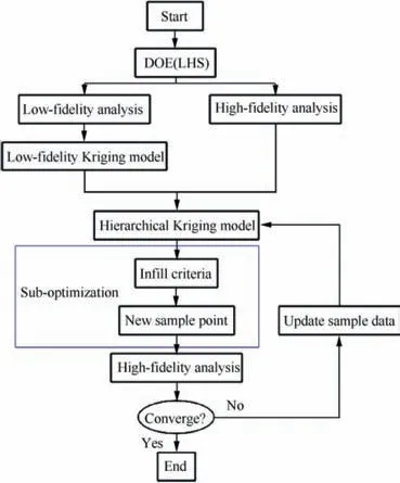
Fig. 1 Optimization procedure.17

3.1. Validation of CFD solver

The Caradonna-Tung rotor in hover57is used as a validation example. The experimental model is a two-blade rotor with a straight blade, and its blade profile is NACA0012 airfoil.The aspect ratio of the rotor is 6 and a chord length 0.1905 m. The calculation status is as follows: Matip=0.877,θ=8°, and Re=3.93×10.6Matipis rotor blade tip Mach number, θ is angle of attack, Re is Reynolds number.

The in-house code ‘‘ROTNS”32,58-60is used as the CFD solver based on three-dimensional Reynolds-average Navier-Stokes equations. The improved Jameson center scheme61is employed for the spatial discretization. The Spalart-Allmaras turbulence model is used for the Navier-Stokes computations.The moving-overset grids are also used, which are composed of body fitted grids around blade and background grids. The body-fitted and body orthogonal C-H grids are used around the blade to take into account the rigid blade rotating motions.The rotor grid is used to simulate the viscous flow and capture the near-field wake vortices. For the grid system in the hovering state, the calculation grid includes two sets: the C-H type rotor grid and the H-H type background grid.

Figs. 2 and 3 show the schematics of the moving-overset grid system and the cross-section of the blade grid, respectively.The 265×68×73 number points of the C-H rotor grid and the 145×89×101 number points of the H-H background grid are used. The comparisons of the pressure coefficient Cpdistribution between calculated and experimental values for five stations are given in Fig. 4. As can be seen, the calculated results are in good agreement with the experimental results,which proves that the CFD method used in this study is reliable.

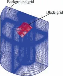
Fig. 2 Moving-overset grid system.

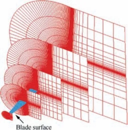
Fig. 3 Cross-section of blade grid.

The UH-60A rotor in hover is added as anther validation example. UH-60A rotor model is a four-blade rotor, it is a blade with a swept tip, and the blade profiles are SC1095/SC1094R8 airfoils. The aspect ratio of rotor is 15.5 and a chord length of 0.527 m. There is about -16° of nonlinear twist. The calculation status: Matip=0.65, Re=6.37×106.For the grid system in hovering, the 265×68×73 number points of the C-H rotor grid and the 145×89×101 number points of the H-H background grid are used.

Fig. 5 shows the comparisons of pressure distribution between calculated and experimental values. CFD result (r/R=0.55,r/R=0.775,r/R=0.92)is in good agreement with the experimental data. Fig. 6 shows change of torque coefficient CQwith thrust coefficient CT, σ is the rotor’s solidity.Fig. 7 shows change of hovering efficiency (FM) with thrust coefficient.CFD result is good agreement with the experimental data. The results proved the correctness of the CFD method used in this paper.

3.2. Validation of noise prediction method

A UH-1H rotor transonic acoustic example is used as a validation example for noise prediction.The experimental model is a two-blade rotor, with a 1/7 ratio reduction, a straight blade,and the blade profile being the NACA0012 airfoil. The aspect ratio of the rotor is13.71, and a chord length is 0.0762 m. The location of the observation point is shown in Fig. 8, R is the radius of the rotor, ω is the rotational speed of the rotor,and the experimental data can be found in Ref.62

The 265×68×73 number points of the C-H rotor grid and the 145×89×101 number points of the H-H background grid are used.The acoustic analogy based on‘‘penetrable data surface-pds” Ffowcs Williams-Hawkings (FW-Hpds) equation is used to compute the noise of the far-filed,providing an accurate prediction for a whole acoustic field. Non-rotating sound source data surface is used as the sound source control surface.It is an individually cylindrical surface.The cylindrical surface and the hub are relatively stationary. The axis coincides with the rotor axis. The tri-linear interpolation method is used to obtain the parameter values of the control surface flow. The data surface radius is 1.2R and the height is 4R. The nonrotating sound source data surface is shown in Fig. 9.

Fig. 10 shows the comparisons of sound pressure between calculations and experiments at the far-field observation points located at (3.09R,0,0) under two conditions: Matip=0.85,Re=1.5×106, and Matip=0.95, Re=1.7×106, respectively.The calculated sound pressure is in good agreement with that in the experimental results,thus proving the correctness of the CFD/FW-Hpdsmethod used in this study.

3.3. Validation of effectiveness of HK model

3.3.1. Example of one-dimensional function

To verify the HK method used in this study,two cases of analytical function tests are introduced in this section. The first is the one-dimensional function test case proposed by Forrester et al.63The high- and low-fidelity function expressions are

The x locations of the high- and low-fidelity samples are S={0,0.4,1.0} and Slf={0,0.2,0.4,0.6,0.8,1.0}, respectively.The optimization problem has an optimal value of f1（x*）=-6.020740 at x*=0.75725.

Fig. 11 shows the High-Fidelity (HF) and Low-Fidelity(LF) analysis functions and the initial sample points. It can be seen that the trends of the two fidelity functions are similar,and their optimal value positions are rather close, which ensures the effectiveness of the established HK model.Fig. 12 shows the prediction results of the Kriging and HK models. Fig. 13 shows the prediction errors of the Kriging and HK models for one-dimensional function. It can be seen that with the introduction of low-fidelity sample points, the prediction results from the HK model are closer to the true function values.Fig.14 shows the optimal convergence curves of the one-dimensional function.When the relative error drops to 10-6(the dotted line in the figure),it ruled that the optimal solution has been found.

Table 1 shows the optimization results of the Kriging and HK models for the one-dimensional function.The results show that the Kriging model and the HK model find the optimal solution to the optimization problem after 25 and 21 iterations, respectively. The optimization efficiency of the HK model is higher than that of the Kriging model.Fig. 4 Comparisons of pressure coefficient distribution between calculated and experimental values (Matip=0.877, θ=8°, and Re=3.93×106).

Fig. 5 Comparisons of pressure coefficient distribution between calculated and experimental values (Matip=0.65, Re=6.37×106).

3.3.2. Example of six-hump camelback function

In addition to the one-dimensional function test case, a sixhump camelback analytical function test case is also analyzed.The high- and low-fidelity function expressions are

Here,the low-fidelity function f2(x)is obtained through the deviation of the independent variable and the linear transformation of the objective function.There are two global optimal solutions for this optimization problem:=（0.0898，-0.7126）and=（-0.0898，0.7126）.The global optimal value isIn addition,there are four local optimal solutions for the function.

Fig. 15 shows the high-fidelity and low-fidelity analysis functions and initial sample points with the numbers of sample points being 5 and 15. The sample data in Fig. 12 are used to build different surrogate models.

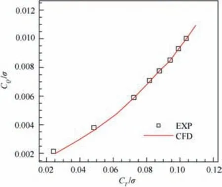
Fig. 6 Change of torque coefficient with thrust coefficient.

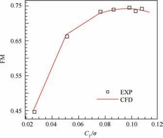
Fig. 7 Change of hovering efficiency with thrust coefficient.

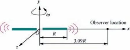
Fig. 8 Location of observation point.

Fig. 16 shows the prediction results of different surrogate models. As can be seen in this figure, the prediction results of the Kriging model are far different from those of the real function, and the prediction results of the HK method are close to those of the real function. Fig. 17 shows the optimal convergence curves of the two-dimensional six-hump camelback function.When the relative error drops to 10-7(the dotted line in the figure), it ruled that the optimal solution has been found.Table 2 shows the optimization results of different surrogate models. Compared to the Kriging model, the HK model can speed up the optimization convergence process,and the value of the objective function in the HK model decreases quickly at the initial stage of optimization iterations.Convergence is quickly achieved. The results show that the Kriging model and the HK model find the optimal solution to the optimization problem after 88 and 44 iterations,respectively. The optimization efficiency of the HK model is higher than that of the Kriging model.

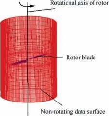
Fig. 9 Non-rotating sound source data surface.

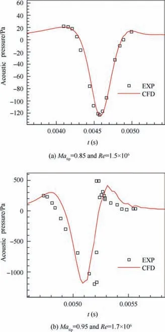
Fig. 10 Comparisons of calculated sound pressure with experimental data for UH-1H rotor.

4. Application of HK model for rotor optimization

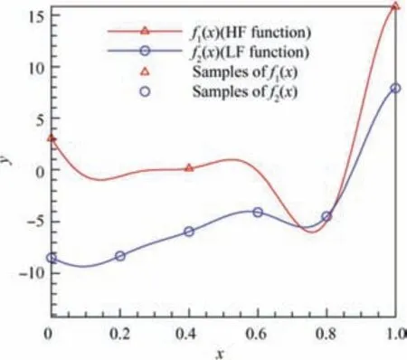
Fig. 11 High- and low-fidelity analysis functions and initial sample points.

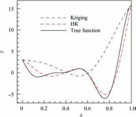
Fig. 12 Prediction results of Kriging and HK models.

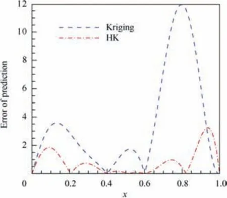
Fig. 13 Prediction errors of Kriging and HK model for onedimensional function.

This study examines the HK-based optimization for the aerodynamic/aeroacoustic performance of helicopter rotors in hover. Since the HSI noise is relatively strong when it comes to high-speed forward flights, most research has studied this noise of the rotor and achieved the effect of noise reduction by weakening shock waves of the blade tip. When the rotor is hovering, the rotational noise, which is a significant part of helicopter rotor noise, becomes prominent in the total noise.This study aims to extend the reduction of rotational noise;therefore,the hover state is adopted as the design state to optimize the aerodynamic/aeroacoustic performance.

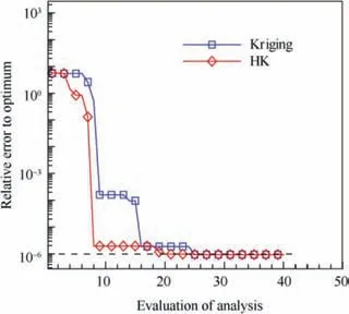
Fig. 14 Optimal convergence curves of one-dimensional function.

It should be noted that the baseline blade used in this example is a practical blade for engineering and has relative low noise characteristics itself. Challenging as it is, the rotor noise reduction can verify the optimization quality of the HK model used in this study.

4.1. Parameterized method and design variables

It has been reported in a previous study29that the rotor blade acoustic characteristics can be improved effectively by including a progressive backward sweep, forward sweep, and taper.A parameterized method for blade planforms that are double-swept and tapered is proposed by learning from the advanced blade shapes. The Class function/Shape function Transformation (CST)64method is introduced to describe the airfoil shape. r/R=0-0.8 is equipped with airfoil with 12% thickness. r/R=0.8-0.9 is equipped with airfoil with 9%thickness,r/R=0.9-1.0 is equipped with airfoil with 7% thickness.

The blade tip of the shape has important influence on the rotor noise65,66; most studies however have optimized only the shape of the blade tip.Although the blade-tip optimization can achieve the effect of noise reduction,it sometimes results in the loss of the aerodynamic performance of the rotor.67,68At the same time, the loss of the rotor’s solidity also causes the drop of the hovering efficiency.To obtain more realistic blade shapes, the entire rotor shape is optimized. Fig. 18 shows 10 Design Variables (DVs) to define the desired blade planform.The four control points in the leading-edge group range from Design Variable 1 (DV1) to Design Variable 5 (DV5), and those in the trailing edge group are from DV6 to DV10.Points DV1-DV5 are controlled with three quadratic function curves,and points DV6-DV10 are controlled with another three quadratic function curves.Tables 3 and 4 shows curves expression for optimal rotor blade. In addition, other four DVs(DV11-DV14) represent the torsion ratio of the blade at the spanwise stations of 0.25R-0.8R, 0.8R-0.9R, 0.9R-R, and the angle of attack of the profile of the blade root section.

Table 1 Optimization results of Kriging and HK models for one-dimensional function.

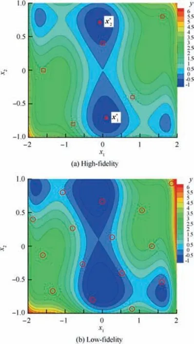
Fig. 15 High- and low-fidelity analysis functions and initial sample points (□and ◦represent positions of sample points at each layer).

The airfoil parameterization uses the sixth-order CST method. The airfoil optimization selects the reference airfoils with three relative thicknesses of 7%,9%,and 12%,and their corresponding stations are at the rotor tip, middle and root section. The number of the DVs of the airfoils is 39, and the number of the total DVs is 53. Table 5 shows design constraints for the relative geometric positions of the DVs. The CST parameterization method uses the Bernstein polynomial as the basis function. Fig. 19 shows the six-order Bernstein polynomial function Si(x). Fig. 20 shows the optimization design space of the airfoil with 9%thickness.The design space ranges of the upper bounds and lower bounds are 2 times and 1/2 times the size of the baseline airfoil, respectively. The design space of the airfoils with 7%and 12%thickness is consistent with that with 9% thickness.

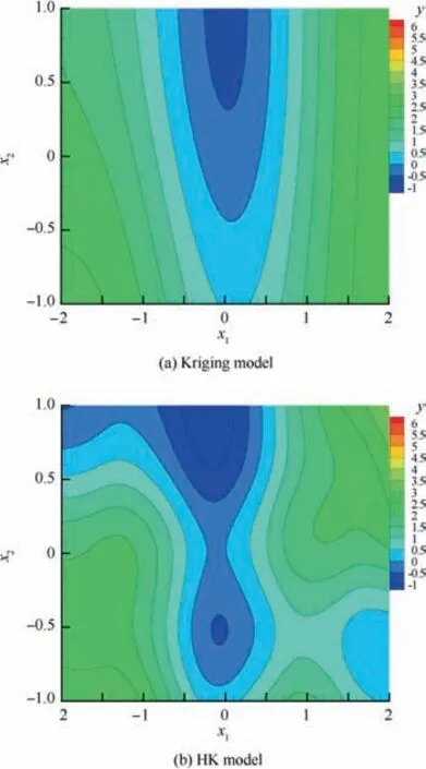
Fig. 16 Prediction results of Kriging and HK models.

4.2. Design objective functions and design constraints

For noise reduction,the absolute value of the minimum acoustic pressure is set as the main objective function.The objective function aims to improve the rotation noise characteristics by reducing the absolute peak of the acoustic pressure at the evaluation points (3.97R, -2R and 0). Fig. 21 shows the location of the observation point.As mentioned above,to obtain more realistic blade shapes,thrust,hover efficiency,solidity and airfoil thickness are taken as the constraints. The objective and constraint functions during the optimization are as follows:

Minimize: ppeak

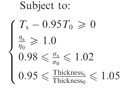
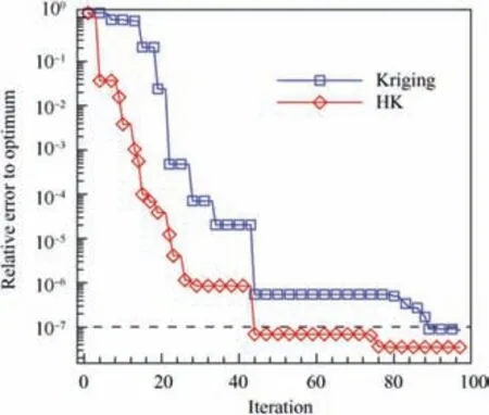
Fig. 17 Optimal convergence curves of two-dimensional sixhump camelback function.

where ppeakrepresents the peak of the acoustic pressure,Ts,ηs,σs,and Thicknesssrepresent the target blade thrust,hover efficiency, solidity, and section thickness of the airfoil, respectively. T0, η0, σ0, and Thickness0represent the baseline blade thrust, hover efficiency, solidity, and section thickness of the airfoil, respectively. Hence, the total number of design constraints is 10. Table 6 presents the calculation status and part of the baseline blade parameters.

4.3. Infill-sampling criterion

In order to expand the applicable dimensions of the SBO method and improve optimization efficiency, this paper proposes a parallel infill-sampling criterion. For the parallel infill sample strategy,five kinds of infill criteria are performed at the same time,which are Minimizing Surrogate Prediction(MSP),Expected Improvement(EI),Probability of Improvement(PI),Lower-Confidence Bounding(LCB),and Mean Squared Error(MSE). The process of the method is as follows: in each iteration step during the optimization process, after the surrogate model is updated, each criterion is independently used to find a new sample point;the newly obtained sample points are allocated to different CPU cores and parallel calculated to get the response values of these new sample points; The new sample points are added to the sample set to enter the next optimization iteration. This parallel infill-sampling criterion have the following advantages:

Table 2 Optimization results of Kriging and HK models for six-hump camelback function.

Fig. 18 Schematic of blade planform with design variables.

Table 3 Leading edge curves expression for optimal rotor blade.

Table 4 Trailing edge curves expression for optimal rotor blade.

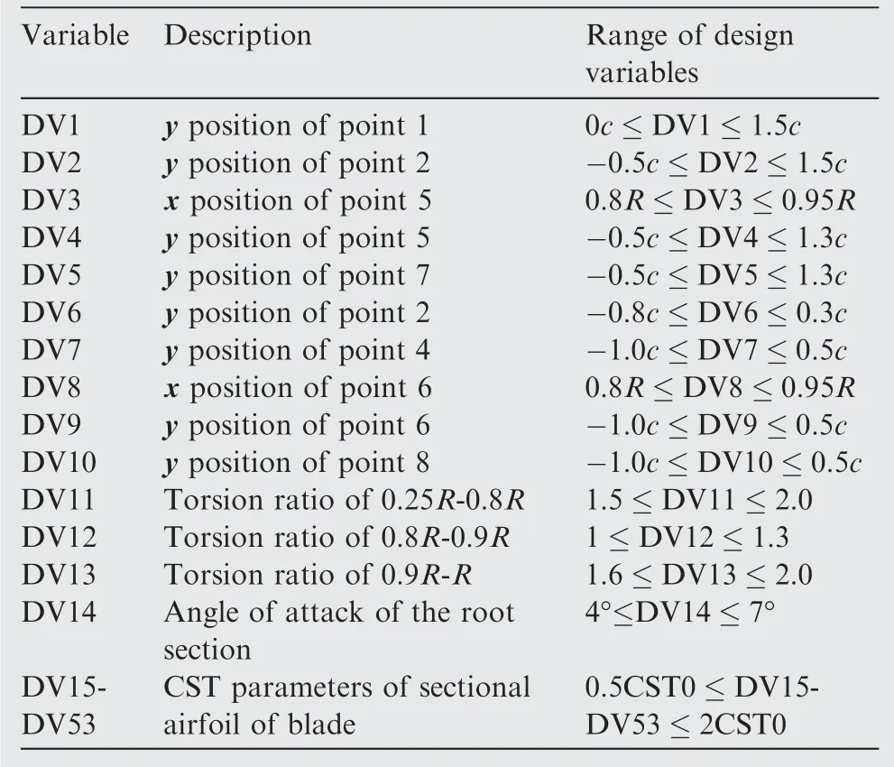
Table 5 Design constraints for relative geometric positions of DVs.

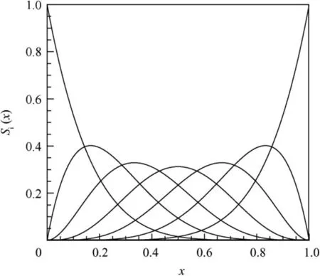
Fig. 19 Six-order Bernstein polynomial function.

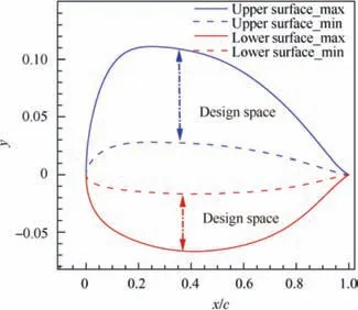
Fig. 20 Design space of airfoil with 9% thickness.

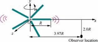
Fig. 21 Location of observation point.

Table 6 Calculation status and part of baseline blade parameters.

(1) Balance of global and local optimization properties.MSE is used to improve the global accuracy of the surrogate model;EI,LCB,PI are used for finding the most likely global optimal solution in the design space; MSP has the local optimization properties,which can be used to find more accurate points near the current optimal solution.The three types of infill-sampling criteria complement each other, so the proposed method is more conducive to find the global optimal solution of the real function.

(2) Five new sample points can be obtained in an optimization iteration,and the response values of the new sample points can be obtained by parallel calculation;when the cost budget is fixed,the number of iterations is reduced,and the optimization efficiency is improved.

4.4. Selection of high-fidelity and low-fidelity analysis models

Latin hypercube sampling is used to generate initial sample points,with 15 high-fidelity and 150 low-fidelity sample points in the two-level fidelity optimization.Due to the large number of low-fidelity sample points and of design variables, a lowfidelity Kriging model is established during each modeling,which is time consuming when low-fidelity sample points are added during the optimization. If there are enough initial low-fidelity sample points, no low-fidelity sample points are added during the optimization. Instead, a low-fidelity Kriging model is established while the initial modeling is optimized,saving the model parameters, and no longer establishing a low-fidelity surrogate model in the optimization process. This greatly saves the modeling time,so that the time for establishing an HK model almost equals that for establishing a Kriging model.

Fig. 22 shows the thrust coefficient and CPU time varied with the number of grids. The grid number 852,544 is set for the low-fidelity computing grid, and the result of the coarse grid is used as the low-fidelity data. The grid number 2,532,156 is set for the high-fidelity computing grid, and the results of the fully converged dense grid are taken as the high-fidelity data.

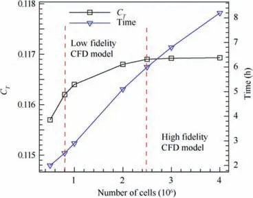
Fig. 22 Thrust coefficient and time varied with the number of grids.

5. Design results and discussion

5.1. Effect of HK model with high dimensional problem

Fig. 23 shows the comparison of the average convergence curve between the optimization of the HK model and that of the Kriging model.The abscissa represents the number of iteration steps, and the vertical axis represents the objective function. Due to the randomness of the surrogate model, the Kriging method and HK method are optimized three times,respectively.The convergence curve is the average of the values three times.

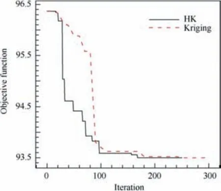
Fig. 23 Average convergence curves of different optimization methods.

Table 7 shows the calculation costs of different optimization methods when the objective is reduced to about 93.5 dB.As can be seen from Fig. 23 and Table 7, the HK model can greatly improve the optimization efficiency when solving high dimensional problems. The results show that the Kriging model finds the objective of 93.5 dB after 248 iterations and the HK model finds that only after 164 iterations. The optimization efficiency of the HK model is significantly higher than that of the Kriging model. Since the HK improves the accuracy of modeling, the number of iterations of highfidelity sample points is reduced during the optimization.When the optimization results are equivalent, the HK model saves 35% of the time used by the Kriging model. It is fully verified that the optimization result of the HK optimization method converges to the result of optimization with only high-fidelity sample points. All the calculations in this study are run on the Intel Core i7 3.4 GHz computer.

5.2. Optimization results and assessment

Fig. 24 shows the shapes and contours of pressure distributions on the upper surface baseline blade and the optimized blade. ‘‘Baseline” in the figure represents the baseline blade and ‘‘Optimized” represents the optimized blade. Table 8 shows part of the design parameters of the baseline blade and the optimized blade. Compared to the baseline blade,the optimized blade has a larger twist angle, its root chord length of the blade is longer, and the tip chord length of the blade is shorter. The optimized rotor swept forward at the middle station of the rotor and backwards at the tip of the rotor. From the theoretical analysis, the sweep of the blade tip in advance and the reduction of the blade tip chord length reduce the rotor noise, thrust and solidity. However, in order to maintain the thrust and solidity of the rotor to satisfy the constraints,the chord length in the middle section of the rotor is increased to add the thrust and solidity.

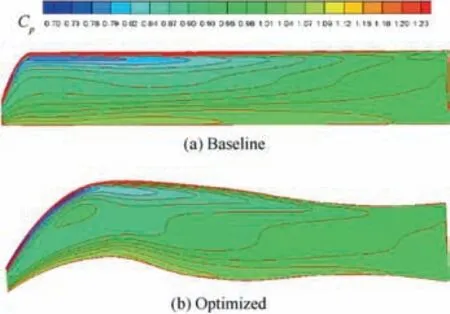
Fig. 24 Shapes and contours of pressure distributions on upper surface baseline blade and optimized blade.

Table 7 Calculation costs of different optimization methods.

Table 8 Part of design parameters for baseline blade and optimized blade.

Fig.25 shows the comparisons of sound pressure p between the baseline blade and optimized blade. Table 9 shows the comparisons of the design objective and constraints between the baseline blade and optimized blade. From Fig. 25 and Table 9, it can be seen that the noise of the optimized blade is reduced by 2.87 dB, becoming much lower than that of the baseline blade.

Figs.26 and 27 show the comparisons of sound pressure of thickness noise and loading noise between the optimized blade and baseline blade.It can be seen that the optimized blade has slight change in thickness noise from the baseline blade (only 0.35 dB), but the loading noise is significantly reduced by 2.38 dB. This is due to the change in the shape near the tip and the load redistribution. Fig. 28 shows comparison of thrust coefficient distribution along rotor blade between the baseline rotor and the optimal rotor, the thrust coefficient of the optimized rotor increases in the middle of the blade and decreases at the tip of the blade compared with the baseline rotor. Since the FW-Hpdsmethod used in this paper can consider the contribution of quadrupole noise,the optimized rotor reduces the quadrupole noise by 0.14 dB. SPL(dB) stands for sound pressure level, the formula is as follows:

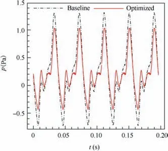
Fig. 25 Comparison of sound pressure between baseline blade and optimized blade.

Table 9 Comparisons of design objective and constraints between optimized blade and baseline blade.

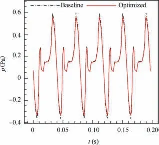
Fig. 26 Comparison of thickness sound pressure between baseline blade and optimized blade.

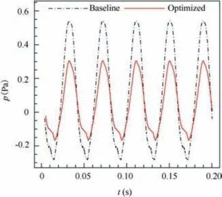
Fig.27 Comparison of loading sound pressure between baseline blade and optimized blade.

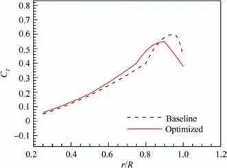
Fig. 28 Comparison of thrust coefficient distribution along rotor blade between baseline rotor and optimal rotor.

Fig. 29 Comparisons of shapes between baseline airfoil and optimization airfoil.

Fig. 30 Comparisons of pressure distribution between baseline airfoil and optimization airfoil.

where pedenotes sound pressure value, prefdenotes reference sound pressure in air, generally pref=2×10-5Pa.

Figs. 29 and 30 show the comparisons of shapes and pressure distributions between the baseline airfoil and optimization airfoil at three spanwise stations with relative thickness ratios being 7%,9%,and 12%.It can be seen that the upper surface camber of the optimized airfoil is reduced, and that the negative pressure peak value of the pressure distribution is weakened and the load is reduced, thereby reducing the noise level when the rotor is in hover.

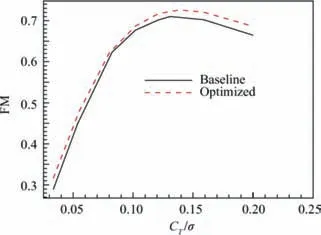
Fig. 31 Comparisons of rotor CT/σ and FM between baseline blade and optimized blade in hover.

Fig. 31 shows the comparisons of the rotor CT/σ and FM between the baseline blade and optimized blade in hover.Fig. 32 shows the comparisons of the rotor CT/σ and SPL between the baseline blade and optimized blade in hover. In general, the optimized rotor has the lower noise level and larger figure of merit at the same CT/σ. The calculation results confirm that the optimized blade has better acoustic characteristics and aerodynamic performance than the baseline blade does.

5.3. Discussion of airfoil for noise reduction optimization

In order to compare the influence of the airfoils on noise reduction in hovering state,the performance assessment is carried out by replacing the optimized airfoils of the blade section with the baseline airfoils while the optimized blade remains unchanged. Fig. 33 shows the comparisons of sound pressure between the baseline blade and optimized blades. The results show that the noise of the optimized blade with baseline airfoils is reduced by 1.80 dB, which means that the optimized airfoils contribute to 1.07 dB for noise reduction. Therefore,the airfoil has a significant influence on noise reduction of the rotor in hover.The influence of the airfoil on noise cannot be ignored.

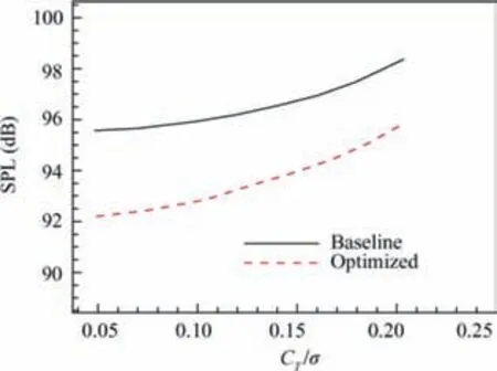
Fig. 32 Comparison of rotor CT/σ and SPL between baseline blade and optimized blade in hover.

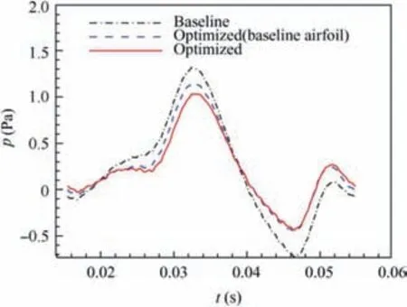
Fig. 33 Comparison of sound pressure between baseline blade and optimized blades.

6. Conclusions

In order to improve the aerodynamic/aeroacoustic optimization efficiency of the rotor blade of the high dimensional problems, the HK model is employed for optimization design in this study. Efficient infill-sampling criterion technique is used to expand the applicable dimensions of the surrogate model.Improved helicopter blade shapes are obtained via numerical optimization, effectively reducing the rotational noise. The quasi-steady method and the FW-Hpdsmethod are coupled with the HK model to perform rotor blade aeroacoustic optimization. Through the analysis of the optimization process and results, the following conclusions are reached:

(1) The optimization method of the HK model can greatly improve the optimization efficiency in solving high dimensional rotor optimization problems. In the case presented, the HK model saves 35% of the time used by the Kriging model.

(2) The high dimensional design variables are used to optimize the rotor blade.The optimized blade noise is significantly reduced by 2.87 dB,much lower than that of the baseline blade under all constraints. The acoustic characteristics can be improved effectively by including a progressive backward sweep, forward sweep, and taper.

(3) The airfoil has a significant influence on the noise reduction of the rotor in hover. The results show that the upper surface camber of the optimized airfoil is reduced.The negative peak value of the pressure distribution is weakened, and the load is reduced, thereby reducing the noise level when the rotor is in hover.In the case presented,optimized airfoils contribute to 1.07 dB for noise reduction.

The future work beyond the scope of this article will focus on perform aerodynamic/aeroacoustic optimization of the rotor blades in hover and forward flight. In addition, LES method, hybrid RANS/LES method will be considered for optimization design work.

Acknowledgement

This research was sponsored by the National Natural Science Foundation of China (Nos: 11772261, 11972305) and ‘‘111”Project of China (No.: B17037).