A new bearing fault diagnosis method based on modified convolutional neural networks

Jiangquan ZHANG, Yi SUN, Liang GUO, Hongli GAO, Xin HONG,Hongliang SONG

School of Mechanical Engineering, Southwest Jiaotong University, Chengdu 610031, China

KEYWORDS Bearing;Convolutional neural networks;Different load domains;Fault identification;Raw signals;Fault diagnosis

Abstract Fault diagnosis is vital in manufacturing system.However,the first step of the traditional fault diagnosis method is to process the signal,extract the features and then put the features into a selected classifier for classification.The process of feature extraction depends on the experimenters’experience,and the classification rate of the shallow diagnostic model does not achieve satisfactory results.In view of these problems,this paper proposes a method of converting raw signals into twodimensional images.This method can extract the features of the converted two-dimensional images and eliminate the impact of expert’s experience on the feature extraction process.And it follows by proposing an intelligent diagnosis algorithm based on Convolution Neural Network(CNN),which can automatically accomplish the process of the feature extraction and fault diagnosis.The effect of this method is verified by bearing data. The influence of different sample sizes and different load conditions on the diagnostic capability of this method is analyzed. The results show that the proposed method is effective and can meet the timeliness requirements of fault diagnosis.

1. Introduction

With the rapid development of industrial internet,it is possible to collect a large amount of sensor data from various machines. The availability of sensor data, which contains information about machine health, has attracted more and more enterprises’ attention. Enterprises want to use datadriven technology to complete the fault diagnosis of machines.1Therefore, in order to maintain industrial machinery working properly and reliably, the demand for intelligent machine health monitoring technique has never stopped.2-4In different types of mechanical components, rolling bearing is the key components of the rotating mechanism, whose health conditions, such as failure diameters at different locations under different loads, can have a significant impact on the performance, stability and longevity of the mechanism.5In order to avoid possible damage, the most common method is to monitor the health status of the mechanism in real time by analyzing the vibration signal.

Aimed to monitor the health conditions of the machinery comprehensively, the installed sensors collect a large amount of signals after a long time. Because intelligent fault diagnosis methods can automatically process signals and identify the health status of the machine,a great deal of research has been made to study these methods. Asr et al.6designed a feature extraction method based on Empirical Mode Decomposition(EMD).The extracted features are input into non-naive Bayesian classifier for intelligent fault diagnosis of rotating mechanism. Georgoulas et al.7proposed a symbolic aggregate approximation framework, extracting features from bearing signals, and then classifying faults by using the nearest neighbor classifier. Xiong et al.8considered that bearing vibration signals have multifractal properties, so multifractal detrended fluctuation analysis is used to extract multifractal features for intelligent fault diagnosis of bearings. Because continuous wavelet transform can overcome the shortcomings of the traditional Fourier transform, Wang et al.9designed a Support Vector Machine (SVM) as a classifier for analyzing vibration signals.

Compared with the traditional machine learning method,deep learning method has achieved good results, but its application in fault diagnosis is still developing. Convolution Neural Network (CNN), as one of the most effective deep learning methods, is also used in fault diagnosis. Because the most common data type is time-domain signal, the onedimensional CNN has been applied to the real-time motor fault diagnosis. In some cases, the data can be presented in two-dimensional format (such as time-frequency spectrum),and then these images can be classified by image processing methods.10-12However, these methods also rely on the knowledge of experts.

Although many of the methods mentioned have achieved good results, there is still much room for improvement. For example, in many studies, classifiers train with very specific type of data, which means that it can achieve high accuracy on similar data while performing poorly on another type.This phenomenon is caused by extracting the error representation feature from the raw signal. In addition, the selection of suitable feature functions requires considerable mechanical expertise and a wealth of mathematical knowledge. On the other hand,due to manual feature extraction and selection,the accuracy of classification results will be unstable when processing different data. Therefore, some studies have suggested that classifiers should be able to classify the data in the original signal directly without feature extraction or manual selection.13-16In other words, the method should be able to process the raw signal automatically and adaptively.And then it should extract the representation feature more precisely.At present,there are three main problems in intelligent fault diagnosis.

First, the unbalanced distribution of mechanical health is not considered. In the real world, the machine works under normal conditions during most of the operating phases.17-19Therefore,data samples from mechanical failures are more difficult to collect than that from normal conditions. Data samples for different mechanical health conditions follow a long tail distribution which means that the data samples of normal conditions are abundant while the fault samples are relatively rare. The unbalanced distribution of data samples forces CNNs to be biased towards the majority health conditions.20As a result, the features of the minority health conditions are learned inadequately, leading to their misclassification.

Second, while many methods can achieve good results in fault diagnosis, there are few ways to directly process the time-domain signal. Most methods have the same classifier,such as SVM and Back Propagation Neural Network(BPNN).This paper focuses on improving feature representation and extraction.

Third, many diagnostic methods have poor domain adaptability.It is not rare for classifiers to be trained with data from one workload and fail to correctly classify samples from another workload.

Aimed to solve the above problems, a Convolution Neural Network with two Dropout layers and two Fully-connected layers (DFCNN) is proposed in this paper. The contribution of this paper is summarized as follows:

(1) A new data preprocessing method is proposed, which converts the one-dimensional vibration signal into twodimensional gray-scale images without any predetermined parameter, and the method can eliminate the influence of expert’s experience as far as possible.

(2) We propose a novel and simple learning framework which uses the time-domain raw signal directly for diagnosis and does not need feature extraction process.

(3) The method has good domain adaptability, and using two dropout layers and two Fully-connected (Fc)layers can easily improve performance.

(4) By visualizing the features that CNN learned,this paper attempts to explore the intrinsic mechanism of CNN model in mechanical feature learning and classification.

2. A brief introduction to CNN

Due to the increasing number of equipment, devices monitoring points and acquisition frequency, a large amount of diagnostic data is obtained, which drives the fault diagnosis field into the ‘‘Big Data” era. CNN, with large data as engine, is one of the best classification methods. This section will introduce the differences between CNN and traditional methods,and briefly introduce the structure of CNN.

The convolutional neural network is a multi-stage neural network consisting of multiple filtering stages and classification stages, and more details on CNN can be found in Ref.21.The purpose of the filtering stage is to extract features from the inputs,which contains two kinds of layers,the convolutional layer and the pooling layer. The classification stage is a multi-layer perceptron consisting of several Fc layers. The function of each type of layer will be described below.

2.1. Difference between CNN and traditional method

According to the research of bearing diagnosis method in recent years,all methods are combined with feature extraction and fault recognition, as shown in Fig. 1. When choosing the BPNN as the classifier, we initially reduce the dimensions of the data, in order to reduce the computational amount and avoid the occurrence of the fitting phenomenon. Using the data-driven feature extraction technology, most of the fault diagnosis models adopt the stacked auto-encoder. Although the step of dimension reduction is eliminated, the signal preprocessing is still needed.

In order to solve above problems, this paper proposes a fault diagnosis method based on CNN structure, which integrates the feature extraction and the fault classification without analyzing the intrinsic mechanism of mechanical device.The time-domain signal is used to diagnose directly, avoiding the problem of information loss caused by preprocessing.

2.2. Design of CNN for bearing fault diagnosis

2.2.1. Convolutional operation

Convolution layer uses convolution kernel to perform convolution operations on the local region of the input signal,resulting in corresponding characteristics. Weight sharing is the most important characteristics of the convolutional layer,which means that the parameters of the convolution window are fixed when each convolution window traverses the entire image. This avoids over-fitting phenomenon caused by the parametric explosions and reduces the memory required for the system to train the network. The first layer is taken as an example. As mentioned earlier, all the units in a feature map share the same set of weights and the same bias so they retain the same feature at all possible locations on the input.The convolution process is described as

2.2.2. Activation operation

After convolution layer processing,the activation layer is used to transform the logit value of each convolution output nonlinearly and to accelerate the convergence of the CNN. Leaky ReLU layers make the weights in the shallow layer more trainable when using back-propagation learning method to adjust the parameters.Select Leaky ReLU as the activation function,and the formula of Leaky ReLU is described as

where kiis a fixed parameter in (0, 1) interval and yl（i，j）is the activation value of convolution layer output y.

2.2.3. Batch normalization

The Batch Normalization (BN)22layer is designed to reduce the shift of internal covariance, accelerate the training process of the deep neural network, improve the network training efficiency and enhance the network generalization ability.The BN layer process first subtracts the mean value μBof the mini-batch from the volume layer input and divides it by the standard deviation. But this will cause the input value to be limited to a small range. Consequently, after standardization,it needs to multiply by a scaling amount γ,plus an offset value β. The input of the batch normalization layer is. The max-pooling transformation is described as follows:

where γl（i）and βl（i）are the scaling and offset of the BN layer respectively,zl（i，j）is the output of the BN layer, and ε is a constant term that guarantees numerical stability.

2.2.4. Pooling layer

It is common to add a pooling layer after a batch normalization layer in the CNN architecture. The pooling layer is operated by the down-sampling operation,and the main purpose is to reduce the parameters of the neural network. In this paper,the largest pooled layer is chosen. For example, its input feature window size is 6×6, and the input feature is down sampled to the 3×3 output feature by a pooling operation with the size of 2×2 and the step size of 2.The max-pooling transformation is described as

where al（i，t）is the activation value of t neuron in l layer of i frame and Pl（i，j）is the width of the pool area.

3. Proposed intelligent diagnosis method

In this section, a novel fault diagnosis method based on CNN is proposed.First,a conversion method is proposed,which can transfer raw vibration signal to images.Then,two dropout layers and two Fc layers are added to the traditional CNN model.

3.1. Data processing

3.1.1. Data augmentation

In order to enhance the feature extraction capability of CNN,the structure is more and more complex,and subsequently,the training parameters are also increasing. However, this structure would easily get over-fitting without sufficient training samples. In the field of computer vision, data augmentation method is used to increase the number of training samples which are able to improve the generalization of CNN.23,24Horizontal/vertical flips, random crops and color jitters are used to increase training samples in the field of computer vision. The augmentation of data is also essential for the high classification accuracy of CNN. It is easy to obtain a large number of training data by dividing overlapping training samples. This process is shown in Fig. 2. For example, a vibration signal with 101,100 points can provide 200 training samples for the DFCNN. When the shift stride is 500, the length of each training sample is 1600.

3.1.2. Signal-to-image conversion method

The traditional intelligent fault diagnosis method is based on the statistical analysis, fuzzy logic expert system or genetic method to extract the features from the raw data.The process of feature extraction relies on experts’experience. In addition,the generality of extracted features is not good. Considering the impact of features on the final results, this paper proposes an effective data pre-processing method, which converts the raw signal of time-domain into an image.This method provides a way to explore two-dimensional features of raw signal.25,26It should be noted that this data pre-processing method can be achieved without any predetermined parameter.

As shown in Fig.2,in this data pre-processing method,the time-domain signals fill the pixels of the image sequentially.A segmentation sample of length K2is randomly extracted from the time-domain signals. Then, an image with pixel point of K×K are obtained by processing the sample. The intercepted signal segments are normalized from 0 to 255,which is just the pixel strength of the gray image. The choice of 160×160 in this paper is dependent on the volume of signal data. L(i)(i=1,2,...,K2) denotes the value of the segment signal. P(j,k) (j=1,2,...,K; k=1,2,...,K) denotes the pixel strength of the image. The process is described as

3.2. Introduction of network structure

CNN has been applied to fault diagnosis.However,compared with the traditional models, the feature extraction ability of these models has not been significantly improved. Most of the models have simple structure, which make them unable to extract the nonlinear expression of the input signal.

The overall framework of DFCNN is shown in Fig. 3. In order to improve the classification accuracy and the adaptability of the structure, two methods are used. First,10×10 sampling points of kernel are adopted in the first convolutional layer. Then, max pooling layer is adopted to reduce the dimension of data. Secondly, two dropout layers and two Fc layers are adopted to improve the adaptability of the network.

3.2.1. Architecture of DFCNN model

The structure composition of DFCNN model is similar to normal CNN models. It is made up of several filtering stages and one classification stage.The main difference is that,in the first convolutional layer, the sampling points of kernels are wide,and the following kernels are with 3×3 sampling points.Then the max pooling layer is used to reduce the dimension of data.Finally,in the classification stage,the logits of the neurons are transformed by Softmax function,which match the probability distribution of different bearing health conditions.

The DFCNN uses wide kernels in the first convolutional layer which have 10×10 sampling points of kernels to extract features.Furthermore,the number of convolution cores in the first convolution layer is relatively less, so as to suppress high-frequency noise. The Visual Geometry Group (VGG)net27performs well with 3×3 sampling points of kernels.Therefore, in order to obtain the useful information of time-domain signals in the middle and low frequency bands,successive small kernels are adopted. And, there are a large number of convolution cores in the second to fourth convolution layers, which helps to obtain features of the time-domain signals and improve the performance of the network. Additionally, the structure composition of model is deeper than the CNN models mentioned before.

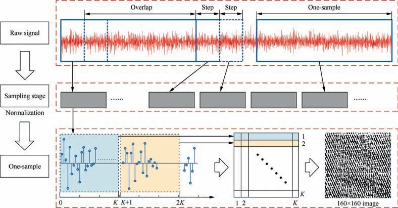
Fig. 2 Signal-to-image conversion process.

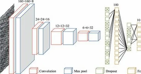
Fig. 3 Structure of DFCNN.

3.2.2. Two dropout layers and two Fc layers

The Fc layer classifies the data with features extracted by the filtering stage,which maps the‘‘distributed feature representation” learned to the label space. The Fc layer uses many neurons to fit the data distribution,but it is sometimes impossible to solve the non-linear problem with only one Fc layer.As the number of Fc layers increase, the non-linear fitting ability of the network can be improved.Then,the dropout layer is added before the Fc layer. This operation means that a randomly selected unit and all its connections are temporarily removed from the model. Its purpose is to provide DFCNN with incomplete signals during training stage, so as to improve the generalization of model. For each new input element, it selects a randomly forming subset of neurons. These subsets use common weights. This operation does not depend on specific neurons and connections, thus solving the problem of over-fitting.28,29The dropout layer is added to the CNN model, which can improve the generalization ability for various classification problems.

So two dropout layers and two Fc layers are adapted in the DFCNN.The length of the first Fc layer is 100,and the length of the second Fc layer is 10.Before using the first and the second Fc layer, dropout operation is performed.

4. Validation of proposed DFCNN method

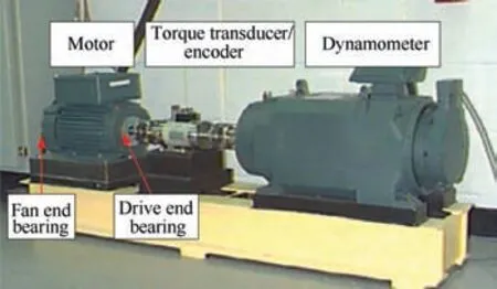
Fig. 4 CWRU bearing fault test-bed.

The experimental data set comes from open source data of Case West Reserve University (CWRU) rolling bearing data center.27At present, the fault diagnosis methods develop rapidly and new theories are constantly being proposed. In order to evaluate the performance of the method proposed in this paper, the standard database should be adopted and the mainstream methods should be used as a comparison.30,31The CNN model is written in MATLAB 2018a with Neural Network Toolbox, and is implemented on a computer where the CPU is Ryzen 5 1600X, the memory is 16 GB, and the GPU is GTX1060.

4.1. Data description

In this experiment, the signal is collected from the drive end bearing as shown in Fig. 4, and the bearing fault is formed by Electrical Discharge Machining (EDM). The raw vibration data are obtained from the motor driving mechanical system by the accelerometers at a sampling frequency of 12 kHz.The test platform simulates four types of faults under different loads.The four different types are the normal state of the bearings, the ball fault, the inner race fault, and the outer race fault.

Data sets A,B,C and D are constructed in 10 different fault categories under different loads (0-3 hp (1 hp=746 W)).Considering the actual situation, the bearing works under different loads,and the data set E is composed of data sets A,B,C and D. Table 1 shows the information of the experimental data sets.Different working conditions of bearings,the normal state of the bearing, the ball fault, the inner race fault and the outer race fault, are represented as Normal, B, IR and OR respectively. The depths of faults are represented as 0.18,0.36 and 0.54 mm.

The size of the converted gray image is set as 160×160,which are processed by signal-to-picture method from a sample signal with 25600 sampling points. Fig. 2 shows signal conversion result under normal work condition and Fig. 5 shows signal conversion results under other nine fault work conditions. As can be seen from the conversion results,the converted images under different work conditions look completely different.

4.2. Compared with other mainstream methods

Taking classification accuracy as an index, DFCNN is compared with several mainstream models. The result shows that,in Table 2, DFCNN achieves better results than these methods.

Table 1 Description of data sets.

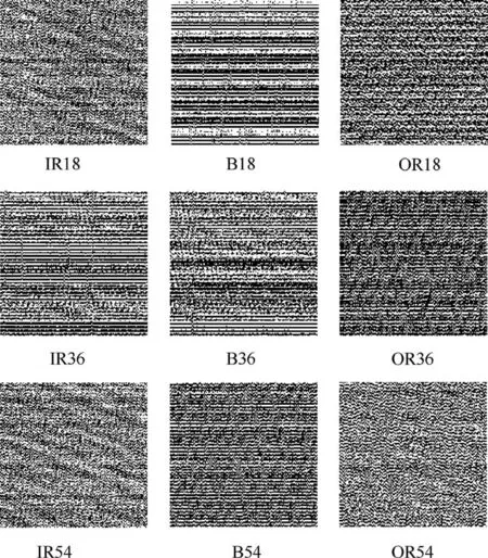
Fig. 5 Converted images under nine fault conditions.

In Ref.33, the multifractal is used to extract fault features,then the SVM classifier is used to classify the data from 10 kinds of fault signals under 0 load,and the classification accuracy of this method is 89.1%. In the same data set, the DFCNN gets 100%accuracy from the time-domain raw data.In Ref.34, statistics method is used to extract the time-domain features. After that, Multi-Layer Perceptron (MLP) is used to classify 6 kinds of faults from three different data sets,acquiring classification accuracy which are 95.7%, 99.6% and 99.4%, while the CNN could still get 100% accuracy from the same data sets. In Refs.34,35, the Deep Belief Network(DBN) method diagnoses faults directly from time-domain raw signals, and the classification accuracy of this method is 98.8% in data set E. The accuracy of the method proposed in this paper has achieved 99.8%, which is much better than the existing methods.

4.3. Effect of data number for training

As a branch of CNN,DFCNN has thousands of parameters to be trained.In order to avoid over-fitting and enhance the generalization ability of DFCNN model,a large number of training samples are needed. The experimental sample is randomly selected from the data set E.The total number of samples were 50, 100, 200, 400, 800, 1600 and the effect of data set size on CNN performance was observed. The initial weights of the CNN model are randomly generated,and the maximum number of iterations is set to 100 times.To verify the stability of the CNN, each experiment was repeated 10 times, and the results are shown in Fig. 6.

The gradient descent algorithm requires the learning rate to be set in an appropriate range. Excessive learning rate may cause instability, while too small learning rate will increase training time.On the premise of ensuring the stability of training,the adaptive learning rate can achieve a reasonable effect.At the same time, it can reduce the training time. Therefore,the initial learning rate is set to 0.0016,and after every 30 iterations, the rate drops to half of its original value.

As shown in Fig. 6, as the number of training samples increases, the classification accuracy gradually increases, and the standard deviation of 10 times accuracy decreases. Even if training samples are relatively small, DFCNN can still achieve a high classification accuracy. The above results show that as the amount of input data increases, the classification accuracy of DFCNN is improved and the ability of feature extraction is gradually enhanced.The increase of training samples can improve the generalization ability of the model.36And the size of training sample does not affect the time required to diagnose a sample. The time spent on diagnosis by DFCNN with different sizes of training samples is shown on the right side of Fig. 6, and the CNN model only needs 1.325 ms to diagnose a sample. DFCNN can meet the real-time requirement of fault diagnosis.

4.4. Performance across different load domains

In this study,the adaptive performance of DFCNN across different load domains was tested, compared with the SVM,MLP and DBN(the data is transformed by fast Fourier transformation).Fig.7 describes the information of training set and test set, and shows the experimental results.

Table 2 Diagnostic results of bearing datasets.

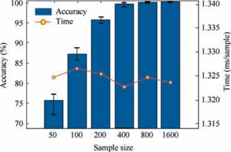
Fig. 6 Number of different training samples, CNN’s accuracy for test set E and time to diagnose individual signals.

The methods of SVM, MLP and DBN have poor adaptability, the average accuracies of the six cases are 66.6%,75.9% and 75.7% respectively. In contrast, the DFCNN method has higher accuracy than other three methods, with an average accuracy of 90.5%. The results show that the features learned by DFCNN from time-domain raw signals have more domain invariance than the traditional features, and the accuracy of each case is more than 80%.

As shown in Fig.8,DFCNN is trained in the data set A and tested in the data set C.The feature representation of the four convolutional layers is reduced to a two-dimensional distribution by t-SNE, as shown in Fig. 8. DFCNN can effectively extract features of data sets with different loads,different fault categories and different fault depths.From Fig.8(a)and(b),it can be seen that the signal features of different fault categories have a high degree of overlap. From Fig. 8(c), the features of different fault types can be clearly classified. However, the features of the same fault at different depths are still in an aggregate state. From Fig. 8(d), the features are highly overlapped of ball fault with a depth of 0.54 mm and inner race fault with a depth of 0.18 mm. The rest of fault features are clearly divided into different areas.

4.5. Necessity of two dropout layers and two Fc layers

In order to verify the effectiveness of the tricks used in the network, the following experiments were carried out to compare the network performance of two dropout layers and two Fc layers, without the first Fc layer and without two dropout layers. In this experiment, the small batch size was set to 20.Fig. 9(a) shows the effect of network training under normal data sets. Fig. 9(b) shows the effect of network training under data set A and testing under data set B.

From Fig. 9(a), it can be seen that under normal circumstances, the total number of training samples is 800, and the convergence speed of the network without the first layer of Fc layer is obviously higher than other models. The classification accuracy is much lower than the other two network structures,because the last BN layer outputs too many parameters,which cause a huge deviation in the automatic feature extraction of the network without the first Fc layer. From Fig. 9(b),it can be seen that when data set is across different load domains, the classification accuracy of the other two models are much lower than that of DFCNN.Without dropout layer,the generalization ability of various classification problems will be greatly reduced in the testing process.

5. Conclusions and future research work

The main contributions of this paper are application of the transformation from signals to images, and then design of a novel CNN network to solve the existing problems in fault diagnosis. DFCNN directly processes the time-domain raw signal without the need of any time-consuming feature extraction process, which reduces the dependence on experts’experience.

Fig. 7 Comparison with SVM, MLP, DBN, DFCNN and DFCNN (Dropout) results under varying load domains.

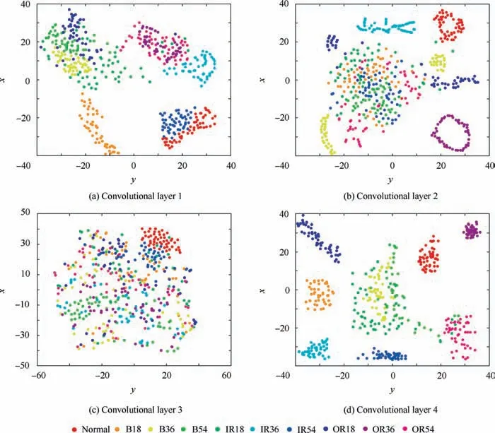
Fig. 8 Visualization under changing data set.

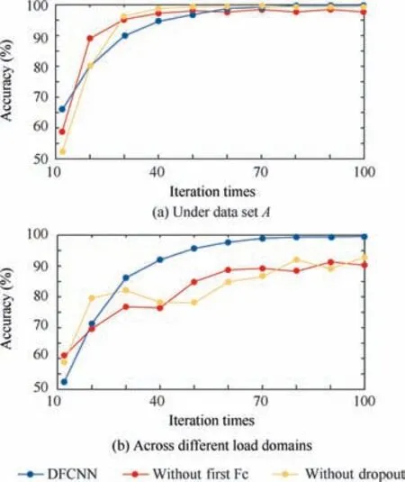
Fig. 9 Accuracy in different conditions.

The results show that although the most advanced deep neural network model has high accuracy for normal data set,its performance decreases rapidly when the workload changes.37,38,13However, DFCNN has a high classification accuracy on normal data, and also has a strong adaptability to workload changes.

Future research can be carried out in the following ways.Firstly, this method can be improved to achieve better adaptability. Secondly, the transfer learning based on CNN can be studied to reduce the training times.

Acknowledgements

Yi SUN and Jiangquan ZHANG contributed equally to this work,as co-first author of this article.Liang GUO and Hongli GAO contributed equally to this work, as co-corresponding author of this article. This research was co-supported by the National Natural Science Foundation of China (No.51775452), Fundamental Research Funds for the Central Universities, China (Nos. 2682019CX35 and 2018GF02), and Planning Project of Science & Technology Department of Sichuan Province, China (No.2019YFG0353).