Estimating interaction between surface water and groundwater in a permafrost region of the northern Tibetan Plateau using heat tracing method

TanGuang Gao,Jie Liu,TingJun Zhang,ShiChang Kang,ChuanKun Liu,ShuFa Wang,Mika Sillanpää,YuLan Zhang

1. Key Laboratory of Western China's Environmental Systems (Ministry of Education), College of Earth and Environmental Sciences,Lanzhou University,Lanzhou,Gansu 730000,China

2.Institute of Water Sciences,College of Engineering,Peking University,Beijing 100871,China

3. State Key Laboratory of Cryospheric Science, Northwest Institute of Eco-Environment and Resources, Chinese Academy of Sciences,Lanzhou,Gansu 730000,China

4.CAS Center for Excellence in Tibetan Plateau Earth Sciences,Chinese Academy of Sciences,Beijing 100101,China

5.Department of Civil and Environmental Engineering Florida International University Miami,FL 33199,USA

ABSTRACT Understanding the interaction between groundwater and surface water in permafrost regions is essential to study flood frequencies and river water quality, especially in the high latitude/altitude basins. The application of heat tracing method,based on oscillating streambed temperature signals,is a promising geophysical method for identifying and quantifying the interaction between groundwater and surface water. Analytical analysis based on a one-dimensional convective-conductive heat transport equation combined with the fiber-optic distributed temperature sensing method was applied on a streambed of a mountainous permafrost region in the Yeniugou Basin, located in the upper Heihe River on the northern Tibetan Plateau. The results indicated that low connectivity existed between the stream and groundwater in permafrost regions.The interaction between surface water and groundwater increased with the thawing of the active layer.This study demonstrates that the heat tracing method can be applied to study surface water-groundwater interaction over temporal and spatial scales in permafrost regions.

Keywords:surface water;groundwater;permafrost;heat tracing method;Tibetan Plateau

1 Introduction

Permafrost, as an integral part of the cryosphere,has undergone unprecedented changes in the past few decades.Significant hydrological changes in permafrost regions have received worldwide attention because water resources and ecosystems are particularly vulnerable to climate change (Benseet al.,2012; Woo, 2012; Walvoord and Kurylyk, 2016;Grenieret al., 2018; Immerzeelet al., 2019). Due to its hydrogeological function as an aquitard, permafrost impacts the movement, storage, and exchange of surface water (SW) and groundwater (GW). Subsurface flow can also influence the state of permafrost by enhancing heat transfer and accelerating thaw (Benseet al., 2009; Chasmer and Hopkinson,2016). Under climate warming, permafrost degradation will likely produce significant changes in surface and subsurface hydrology concomitant with modifications to the hydrological framework, particularly the SW-GW exchange which correlates with water-heat interaction processes (Careyet al., 2013;Wellmanet al., 2013; Kurylyket al., 2014). The SW-GW exchange directly reflects the effects of permafrost thaw on hydrological processes, such as subsurface flow paths, residence time, and partitioning of water stored above and below ground. Therefore,understanding the interaction between hydrological changes and permafrost thaw is essential to reduce uncertainties in predicting the responses of water resources and aquatic ecosystems to climate change in the high altitude regions (Chenget al., 2014;Abbott and Jones,2015).

Recently,many scientists have investigated hydrological regimes in mountainous permafrost regions(Yeet al., 2009; Liuet al., 2011; Cheng and Jin,2013; Cuoet al., 2013).Although explanations of the linkage between permafrost thaw and hydrological processes abound, the logistical challenges of measuring and monitoring subsurface water fluxes and storage in permafrost regions limit the predictions of how future climate change may influence hydrological conditions in these regions (Walvoordet al., 2012; Walvoord and Kurylyk, 2016). Furthermore, existing modeling studies of increases in baseflow and subpermafrost flow are based on hypothetical scenarios(Geet al.,2011;Benseet al.,2012).

Heat tracing method has been used firstly to identify and quantify reach-specific SW-GW interactions in humid environments (Constantzet al., 2013; Irvineet al., 2017). Because of conduction and convection,heat is a naturally occurring tracer in stream systems,with daily temperature fluctuations within an SW body leading to thermal responses in the sediments at the SW-GW interface (Constantz, 2008). By measuring streambed temperatures in an environment with significant differences between groundwater and surface water temperatures,the propagation of a heat signal by conductive and convective heat fluxes can be used as an indicator to reveal exchange flow directions or to quantify exchange fluxes (Hatchet al.,2006; Keeryet al., 2007). With recent developments in measurement and logger technology, it is now a common practice to use analytical approaches to interpret temporal and spatial dynamics of water fluxes from multilevel temperature records (Rauet al.,2014).

The Tibetan Plateau is considered as the "Asian Water Tower" and is particularly important in the regional water cycle and ecosystem (Yaoet al., 2012;Immerzeelet al., 2019). The discontinuous mountainous permafrost region in the northern Tibetan Plateau presents an excellent testbed for the heat tracing method since the SW-GW interactions are generally different for river reaches in areas with and without permafrost.This study aims to investigate the feasibility of using the heat tracing method to identify exchange flow patterns at the SW-GW interface and test the validity of heat tracing methods in permafrost hydrology. Specifically, a one-dimensional convectiveconductive heat transport equation combined with data collected by the fiber-optic distributed temperature sensing (FO-DTS) method was used to trace the heat exchange between SW and GW. The results demonstrate the capability of the heat tracing method to help understand the SW-GW interaction in permafrost environments.

2 Methodology

2.1 Study area

The hydrology in discontinuous permafrost regions appears to be particularly sensitive to natural or anthropogenic-induced climate changes, because of the potential flow exchanges between the water of suprapermafrost and intrapermafrost zones, or with water in non-permafrost areas (Woo, 2012).The Yeniugou (YNG) Basin is located at the upper reaches of the Heihe River of the Qilian-Altun Mountain discontinuous permafrost region in the northern Tibetan Plateau (Figure 1). It covers an area of approximately 5×103km2as a narrow basin stretching 160 km along the Heihe valley,with a width less than 60 km.Elevations range from 2,615 to 4,876 m a.s.l., with a mean elevation gradient of 14 m/km. Fifty-six small glaciers (with a total area of 11.34 km2) are distributed at higher elevations (above 4,500 m a.s.l.) on both sides of the Qilian Mountains (Huaiet al., 2014).Glacial meltwater contributes about 3.6% of the total river runoff (Chenget al., 2014). The mountainous permafrost area occupies approximately 68% of the YNG Basin, according to the 1:4,000,000 Frozen Ground Map in China (Wang, 2006). Measurements from 18 boreholes drilled in the YNG Basin show that the thickness of permafrost ranges from 0 to 113 m(Wanget al.,2013).

Atmospheric circulation patterns over the Tibetan Plateau are dominated by Indian monsoon in summer and the Westerlies in winter (Yaoet al., 2012). The mean annual air temperature in the area is less than 2 °C, and the mean annual precipitation ranges from approximately 250 mm to 500 mm in the upper reaches of Heihe River (Gaoet al., 2016). Snow-covered areas exceed 40% of the YNG Basin in winter; however, snow-cover days constitute less than 10% of the year, except on glaciers and perennially snow-covered areas(Biet al.,2015).

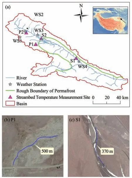
Figure 1 (a)Location of the Yeniugou(YNG)Basin in the northern Tibetan Plateau and the hydrometeorological measurement sites(S1,S2,P1,and P2),and the extent of FO-DTS measurement sites at P2(b)and S1(c)

2.2 Heat tracing method

The principle of the heat tracing method is that the daily temperature fluctuations caused by solar radiation within a SW body lead to temperature responses(because of conduction and convection) in the sediments at the SW-GW interface (Constantz, 2008).However, temperature gradient measurements beneath the streambed combined with an analytical or numerical heat transfer model can only estimate point groundwater discharge(Rauet al.,2015).The application of distributed temperature sensors along river reaches can identify large spatial variations, therefore significantly increasing the spatial and temporal scale of temperature observations (Selkeret al., 2006;Hatchet al.,2010;Krauseet al.,2012).However,this method cannot provide estimations of groundwater directly.In this study,we use an integrated approach that consists of distributed measurements of temperature and its gradient to investigate the SW-GW interaction.

2.3 One-dimensional heat transport equation

The one-dimensional (1-D) convective-conductive heat transport equation (1-D HTE) has a sinusoidal temperature boundary at the top and a constant temperature boundary at infinite depth. The streambed vertical fluxes are calculated by the extracted daily sinusoidal component of temperature(Rauet al.,2015).The 1-D heat convection conduction equation is(Equation(1)):

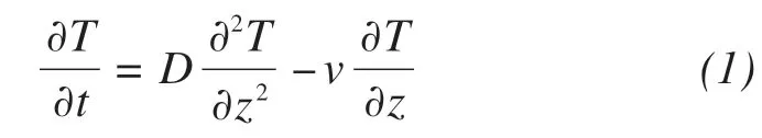
whereTis temperature,tis time,Dis the effective thermal diffusivity,zis depth, andvis the thermal front velocity(Suzuki,1960).

Stallman (1965) derived a solution for (Equtaion(1)) requiring two temperature time series recorded at different vertical positions, which allowed for the evaluation of flow velocity from the damping of temperature amplitudes and phase shift.Based on the subsequent development and expansion of Stallman's solution (Gotoet al., 2005; Hatchet al., 2006; Gordonet al., 2012), McCallumet al.(2012) extracted a system of equations that explicitly solved the thermal front velocity from consecutive pairs of temperature amplitude and phase shift data. The thermal front velocity is defined as(Equation(2)):

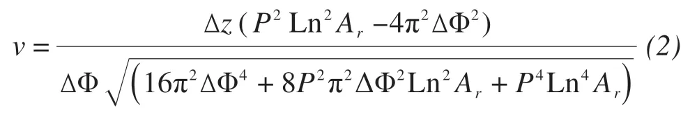
wherevis the thermal front velocity (m/d), Δzis the spacing between measurement points (m),Pis the period (d),Aris the amplitude ratio, and ΔΦ is the phase shift of temperature maxima(d).

Typically, the SW-GW interaction is quantified by Darcy velocity (q), which equals the estimated thermal front velocity (v) multiplied by a constant (γ,Equation(3)):

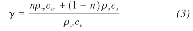
Whereγis the Darcy velocity index,nis porosity,ρwandcware the respective density (kg/m) and heat capacity(J/(kg·°C))of water;andρsandcsare the density (kg/m) and heat capacity (J/(kg·°C)) of a solid,respectively.

The analytical solution of 1-D HTE is based on an assumption of steady-state fluid flow (Stallman,1965), which contrasts with the natural processes that are commonly transient. Lautz (2012) and Rauet al.(2015) have shown that the quantification using heat tracing methods based on the assumed harmonic temperature data can potentially lead to flawed flux estimates.To avoid the heterogeneity of the local thermal physical parameters such asγ,we only used the direction and variation of the thermal front velocity, which can reveal the SW-GW interactions. In this study, the sign convention forvis as follows: positive indicates gaining water,and negative means losing water.

A semi-automated computer program was developed for deriving amplitudes and phases from the temperature data to delineate the noise in the signal since conventional signal-processing methods introduce erroneous temporal spreading of advective velocities and significant anomalies (Rauet al., 2015). The program selects the peak temperature and corresponding time in one temperature cycle based on diurnal fluctuations, followed by automatic selection of subsequent peaks and time across the remaining records. If the time corresponding to the maximum and minimum values does not fall within 24 hours, the program sets the phase and time as null values.

2.4 Fiber-optic distributed temperature sensing(FO-DTS)

Selkeret al.(2006) presented the first hydrologic application of a vertical high-resolution DTS system.Since then, this technology has been gained wide use in observing a broad range of hydrologic processes(e.g., Tyleret al., 2009; Liuet al., 2016). The FODTS measurement is based on the analysis of the temperature-dependent Raman spectra backscatter properties of a laser pulse that is applied to, and propagates through, a fiber-optic cable (Selkeret al., 2006). The backscattered light is spread across a range of wavelengths, some of which are affected by temperature changes while others are immune. This shift in the light wavelength is referred to as the Raman effect;the light with wavelengths above the incident light is the Raman Stock signal and the light with wavelengths below the incident one is the Raman anti-Stokes signal. By precisely measuring the difference in the signal intensity of the backscattered light, accurate temperature measurement can be obtained.

Laueret al.(2013) systematically investigated the capability of the FO-DTS to identify or estimate groundwater discharge from discharge points and found that its result was reliable when the contrast between groundwater and surface water temperatures exceeded a certain threshold.The strength of the temperature anomaly (AT) was used as an indicator of the temporal variability of these signals.ATis defined as the difference between a local temperature measurement at a specific point and the spatial average temperature of the cable section within the streambed(Equation(4)).

WhereATis the strength of the temperature anomaly,is the spatial average temperature of the cable section within the streambed (°C), andXiis the measurement location along the cable.

The variability ofATis described by its temporal standard deviation(STDEV)(Equation(5)):

WhereXitis the measurement location at timet,AVHGis the strength of vertical hydraulic gradients anomalies.

2.5 Field observation system

Streambed temperature data were collected from instruments hung in steel piezometers with an inner diameter of 8 cm driven 80 cm below the surface of the streambed. A screen with openings of 0.5-cm diameter allowed free flow of water into or out of the piezometer and good thermal contact between the sensors and the streambed.

Four piezometers were installed at approximately 1 m from the riverbank in areas with and without permafrost (S1 and S2 in areas with seasonally frozen ground, and P1 and P2 in areas with permafrost) and removed after measurement (Figure 1). The data was recorded at 15-min intervals with a HOBO®water temperature logger(Water Temp Pro v2,±0.21 °C precision, Onset, Bourne, MA, USA) at 0, 20, and 50 cm depths from July to September, 2015. An automatic water-level meter (Levelogger Model 3001 F2/M2,±0.1 cm precision, Solinst Canada Ltd., Ontario, Canada) was installed near S1 and also recorded water levels at 15 min intervals by a pressure gauge (Solinst Barologger,±0.05 kPa precision).

A 500-m ruggedized fiber-optic cable with two 50-μm multimode fibers was secured on the streambed approximately 1 m from the riverbank using approximately 100 tent pegs.Notably,the fiber-optic cable was attached to the pegs via plastic ties to avoid preferential heat conduction along the metal pegs. In addition, cobbles were used to anchor the cable to the streambed.

The accuracy of fiber-optic temperature measurement is controlled by the total number of photons detected as a function of integration time and spatial integration length (Roseet al., 2013). The selected FODTS system(AP Sensing,Böblingen,Germany)is capable of measuring temperature with high precision at 15 min intervals with a spatial resolution of 0.25 m using couple-ended measurements. To account for temperature offset and instrument drift, a 30-m section of the cable was coiled and placed in an insulated box filled with water together with a PT100 temperature probe for reference; the cable was set for six hours to achieve thermal equilibrium during system maintenance and recalibration.Temperature data was continuously collected along the DTS cable over a 48-hour period (September 23-25,2015 at S1;September 21-22,2015 at P2).

The precision of the FO-DTS declines as signal strength decreases (Tyleret al., 2009; Roseet al.,2013). The FO-DTS system can automatically calibrate the sensor cable in temperature offset and enhance the attenuation ratio by using the external temperature probe and the built-in program. Note that the reference temperature probe was in the same area as a specific segment of the sensor cable (called a reference loop) to obtain the exact temperature for reference. Double-ended calibrations were conducted to offset signal loss along the cable length. The measurement precision of temperature after calibration was±0.12 °C.

From 2012 to 2014,Wanget al.(2013)and Gaoet al.(2016) established 18 monitoring boreholes installed with a string of thermistors spaced at 0.5-m intervals to record temperature in areas with and without permafrost in the YNG basin. The soil temperature data was collected at depths ranging from 0.5 to 10 m below the natural ground surface. Notably, the thermistors,made by the State Key Laboratory of Frozen Soil Engineering, had an accuracy of ±0.05 °C.For this study, three of these boreholes that were near the streambed temperature observation sites (S2, P1,and P2) were chosen to carry out in-situ measurements manually for two or three times on June 18,August 9-10,and September 25-26 in 2015.

Three automatic weather stations (Campbell, USA)near the piezometer and borehole sites (WS1, WS2,and WS3 in Figure 1) provided meteorological data at 30-min intervals.A manual observation station (WS4,Figure 1) belonging to the National Meteorological Network of China (elevation 3,320 m a.s.l.) also collected data from use in this study.

3 Results

3.1 Streambed and permafrost temperatures

Streambed and permafrost temperatures are valuable background information for analyzing the SWGW interaction.Figure 2 shows the boxplots of streambed temperatures measured at depths of 0, 20 cm, and 50 cm of S1,S2,P1,and P2.The streambed temperature remained low in the YNG Basin (5-10 °C, Figure 2). The streambed temperature varied from -2 to 22 °C during the observation period; diurnal oscillations ranged from 2 to 22 °C. Damping existed in the stream signal at the sites of S1, S2, P1, and P2, with the greatest damping at P2 and lesser damping at P1.The damping indicated the heterogeneous nature of the local physical and thermal properties.

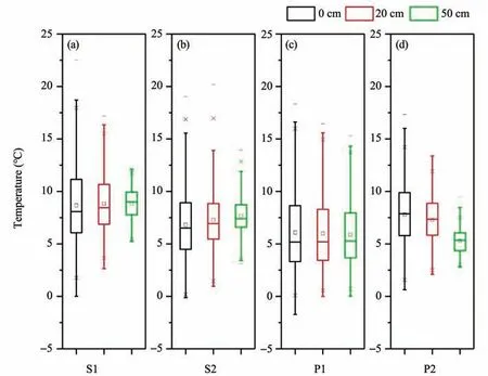
Figure 2 Boxplots of streambed temperature data at depths of 0,20 cm,and 50 cm of(a)S1,(b)S2,(c)P1,and(d)P2 during July to September 2015

In the streambed at S1, the temperature at a depth of 0 cm was the greatest with a mean value of 8.67 °C and a range of 0.01-22.3 °C. The site at P2 had the second-largest mean value of 7.79 °C with a range of 0.63-17.35 °C. In the streambed at P2, the mean temperature at 0 cm was higher than that at S2 and P1. The mean temperature at a depth of 50 cm varied significantly across sites (8.83 ° C at S1,7.67 °C at S2, 5.89 °C at P1, and 5.39 °C at P2)which was consistent with the elevation gradient between sites.

Figure 3 shows the soil temperature at depths of 0-10 m measured in boreholes near S2, P1, and P2.The temperature data indicated that S2 were free of permafrost, while P1 and P2 were located in warm permafrost (≥-1.5 °C).Assume late September as the time of maximum thaw, the active layer thickness(ALT)was calculated with the temperature data by interpolation (Brownet al., 2000). It was found to be 1.54 m and 2.78 m at P1 and P2,respectively.

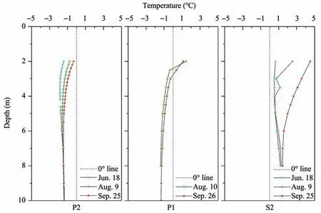
Figure 3 Soil temperature data from boreholes near the streambed temperature observation sites(P1,P2,and S2)on June 18,August 9-10,and September 25-26 in 2015

3.2 Temporal patterns of SW-GW interactions

According to the 1-D THE (Equation(2)), the mean thermal velocities depend on the physical and thermal parameters of individual observation sites and varied from a maximum of-3.12 m/d at P1,to a minimum of -0.67 m/d at P2. The streambed at P1 was coarse-grained, which could possess higher porosities and lower sediment densities and heat capacities,while the streambed at other sites was relatively finegrained. The negative thermal front velocities indicated that the stream was losing water at all observation sites (with or without permafrost) during the ground thaw season(Figure 4).

The temporal changes of thermal velocities revealed a significant difference between seasonally frozen ground and permafrost sites.The thermal velocity trends at S1 and S2 were not substantial, while those at P1 and P2 showed a significant decrease over time,with a rate of 0.13 cm/d and 1.38 cm/d,for P1 and P2,respectively. The different trends indicated that the patterns of SW-GW interaction were closely related to whether permafrost exists in the sites.

3.3 Spatial patterns of SW-GW interactions

The FO-DTS temperature surveys were carried out at S1 and P2 in September 2016 (Figure 5). The observed temperature revealed that stream warming occurred from 09:00 until 16:00, and cooling occurred from 16:00 to 09:00 of the next day, consistent with the piezometer measurements. The temperature of the water column at P2 was lower than that at S2 because the water column at P2 was shallower than that at S2. The temperature changes at the bottom of the surface water column varied less than 0.06 °C along the investigated stream reach.

An analysis of the strength of temperature anomaliesAT(xi) revealed a largely homogeneous temperature pattern in the streambed, with a temperature variability of up to 0.7 °C at S1 (Figure 6a). The typical temperature variations around the spatial average were±0.4 °C.There were no distinct cold spots or large temperature variations (STDEV) along the cable at S1, indicating that there was no up-welling of groundwater.Two warm places were identified without temporal persistence,probably due to shallow water blocked by rocks.

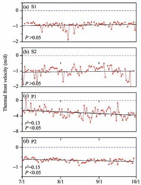
Figure 4 Thermal front velocities and their trends from July to September in 2015 at(a)S1,(b)S2,(c)P1,and(d)P2 along Yeniugou stream.The dashed blue lines represent a thermal front velocity of zero,and the black lines are the best linear fit

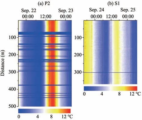
Figure 5 Riverbed temperature variations measured by FO-DTS at(a)P2 from 19:00 September 21 to 03:00 September 23,2015 and(b)S1 from 15:00 September 23 to 07:00 September 25,2015

The strength of temperature anomaliesAT(xi) and their temporal standard deviations (STDEV) at P2 also showed homogeneous temperature patterns in the streambed (Figure 6b). The temperature anomalies were less than 0.25 °C,and the STDEV was near 0 °C.Some slight cold spots were identifiable in the temperature anomaly plot. Nonetheless, they can be considered to be the uncertainty of the data collected by FODTS rather than the influence of cold groundwater,since heat conduction and streambed topography could result in up to 0.3 °C in temperature anomaly(Krauseet al., 2011). Both the low STDEV and small temperature anomalies imply that there was no colder up-welling groundwater in the observation reaches,and possibly indicate the bypassing of regional groundwater due to preferential lateral flow or confined streambed structures beneath the investigated zone of(Krauseet al.,2012).

4 Discussions

4.1 Implications of SW-GW interaction in permafrost region

The thermal velocity trends demonstrated that the SW body tended to lose more water overtime in the permafrost areas (P1 and P2), therefore resulting in the thickening of the active layer. In contrast, the hydraulic condition in the permafrost-free area varied but exhibited no trends. Careyet al.(2013) and Quinton and Baltzer (2013) suggested that the thickening active layer could lead to decreases in the bulk hydraulic conductivity and the hydraulic gradient. Thus,the increased amount of water lost into permafrost was mainly the result of the increases in soil drainage(Walvoordet al.,2012)and the enhancement in suprapermafrost transmissivity due to the thickening countered by reductions in the bulk hydraulic conductivity.The intensity of the SW-GW interaction in the area without permafrost fluctuated but exhibited no trends in summer.This observation was consistent with studies using chemical and isotope analyses in a boreal catchment that indicated the thickening of the active layer could transmit more water through a zone of lower hydraulic conductivity (Quinton and Baltzer,2013;Kochet al.,2014).In summary,the heat tracing method can provide direct evidence for the dynamic SW-GW interaction in the permafrost area.

The water loss condition indicated that the groundwater table becomes deeper beneath the SW body according to 1-D THE,and the small temperature anomalies observed by FO-DTS implied no groundwater inflow to the SW body. Altogether, it demonstrated the low connectivity between the stream and the underlying aquifer. The changes in the relative connectivity between the stream and the underlying aquifer can influence the SW-GW interaction (Hatchet al., 2010).Permafrost can act as an impermeable layer that limits infiltration, storage, and connectivity with the deeper regional flow. Consequently, it could lead to a higher hydraulic head in the subpermafrost aquifer and lower hydraulic head in the suprapermafrost aquifer (Woo,2012). Later in the thawing period, as the active layer thaws and groundwater table deepens beneath the stream,permafrost-area reaches which lose water may become more disconnected between the surface water and groundwater.It should be noted that not all reaches in the YNG Basin experienced losing conditions.Based on field observations, there were some instances of up-welling groundwater in the streambed near the lower boundary of permafrost. The result from isotopic tracer analyses performed by Liet al.(2016a, b) in other upper Heihe River sub-basins indicated that water from the active layer accounted for 9%-29% of the total runoff in July. Unfortunately, these reaches were not suitable for the FO-DTS observation because of the braided nature of the stream at these locations.

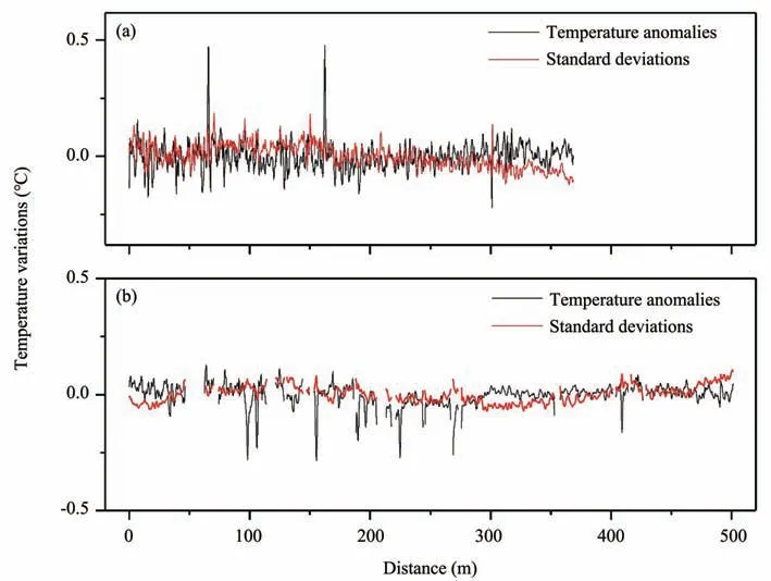
Figure 6 Temperature variability along the cable obtained by FO-DTS at S1(a)and P2(b)

The approach presented in this study extends the current knowledge accumulated from point-in-time or point-in-space measurements (Tyleret al., 2009). It can provide an understanding of SW-GW interaction in permafrost regions for a broad range of temporal and spatial scales. This approach also supports the identification of spatial patterns and temporal distribution of the SW-GW interaction.

4.2 Limitations and uncertainties in permafrost region

The combination of FO-DTS derived streambed temperatures with HTE temperature gradients provided a powerful indicator of the SW-GW exchange.However, there were still limitations and uncertainties with this approach,particularly in permafrost regions.

4.2.1 Limitations

The harsh cold environment made very high demands of the measurement devices in terms of accuracy, measurement range, and service life. Field measurements (Figure 7) showed that the streambed temperatures in permafrost regions could fall below 0 °C in summer from July to September in 2015, with air temperature variations of up to 28°C.

The permafrost region was characterized by the intensified occurrence of freeze-thaw and severe frost action. FO-DTS cables were installed at seven different sites for observing temperature-depth variations in the study area,three of which failed due to frost heave damage. Even in the sites where the sensors survived the harsh environment (e.g., S1), the system produced abnormal data due to freeze-thaw cycles, as indicated by the blue boxes in Figure 7.

The development of low-cost, accurate, and reliable miniature temperature recorders has facilitated the measurement of stream temperatures (Webbet al.,2008). Theoretically, the FO-DTS method has a high temporal and spatial resolution, which generally exceeds that of the traditional point-in-time or point-inspace measurement (Tyleret al., 2009). However,the long-term temporal repeatability of DTS systems is unknown and is an area of future study. The DTS system remains very expensive for research applications,and the environment for hydrologic applications is more complicated than that for industrial applications.

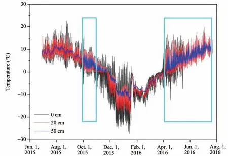
Figure 7 Stream temperature data at depths of 0 cm,20 cm,and 50 cm of S1 from July 2015 to July 2016.The blue boxes indicate the abnormal data in the measurement period

4.2.2 Uncertainties

Our computer program directly extracted sinusoidal temperature signals from noisy raw records without filtering to avoid erroneous temporal spreading of advective velocities and significant anomalies induced by signal-processing techniques, such as Fourier transform and Dynamic Harmonic Regression(Hatchet al., 2006; Keeryet al., 2007).As a result of energy decrease with depth,some low energy oscillations became linear (i.e., lack of sinusoidal signal).There were 13 days without a sinusoidal signal at P2,eight days at S2, and six days at S1, which corresponds to 14.1%, 8.7%, and 6.5%, respectively, of the observation days. Thus, the cold environment in permafrost regions can result in many days absent of a sinusoidal signal at some depths. For example, the air temperature recorded at 15 min-interval at P2 showed that the air temperature could fall below 0 °C, even in August. The days without a sinusoidal signal occurred when extremely low temperatures occurred at night, or low temperatures existed during the daytime(Figure 8).

System responses to sudden water fluxes may introduce errors. The temporal patterns of the changing thermal velocity can take place in association with short-term increases in channel discharge (Hatchet al., 2010).This phenomenon was also observed at S1,where sharp water loss followed a high water-level condition (Figure 9). McCallumet al.(2012) concluded that rapid changes in hydraulic forcing (i.e.,floods)could lead to erroneous fluxes because of a violation of the method's assumptions. Furthermore, a reversal in the flux direction,as expected during flood events (e.g., the nature of the flood hydrograph as well as return flow to bank storage), complicates the systemꞌs thermal response. Thus, the use of heat tracing methods based on the assumption of harmonic temperature data could lead to potentially flawed flux estimates(Rauet al.,2015).

The physical and thermal properties of streambed could limit the application of the heat tracing method in permafrost regions.Thermal conductivity is virtually independent of streambed texture, whereas hydraulic conductivity is highly sensitive to streambed texture (Stonestrom and Constantz, 2003; Rauet al.,2010). This observation was based on the fact that heat travels in a direct path through the entire crosssection of solids and pore-filling fluids, whereas fluid flow finds its way through a tortuous path formed by interconnected pores.Fluid flow is the product of hydraulic conductivity and hydraulic gradient (Darcy's law). Analogously, conductive heat flow is the product of thermal conductivity and temperature gradient(Fourier's law). However, it is difficult to accurately estimate the physical and thermal parameters, particularly in the rough river course of the permafrost re-gion. This difficulty forces many heat-tracing study groups to use reference values obtained in the laboratory, which could lead to a large variation in the results. For example, McCullumet al.(2012) used the thermo-physical property values reported in the literature in a Monte-Carlo analysis and reported a 3-fold difference between the maximum and minimum Darcy velocity.

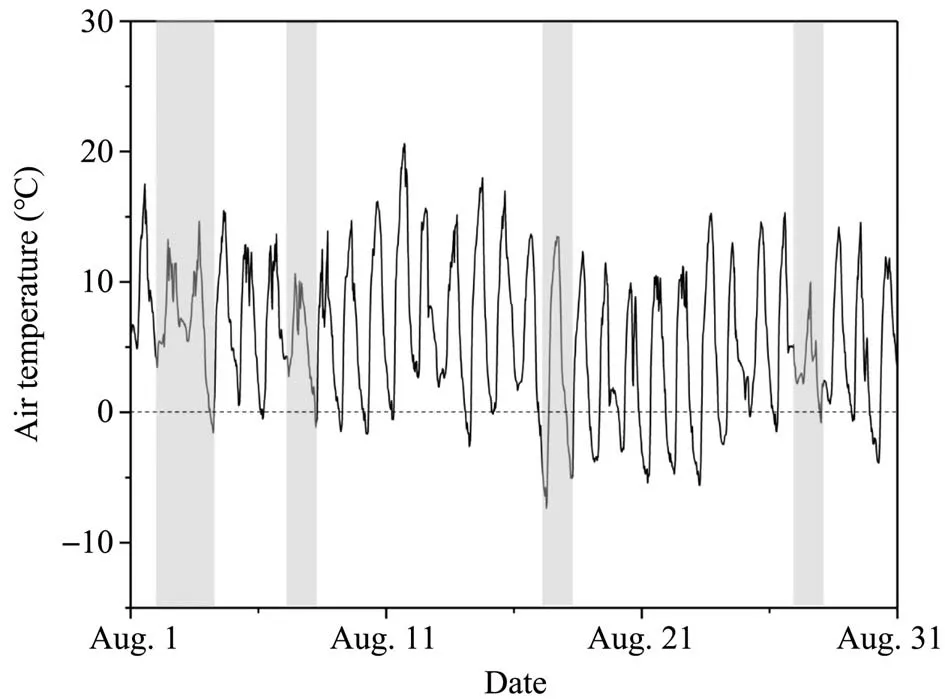
Figure 8 Air temperature recorded at P2 in August 2015.Grey rectangles indicate days without a sinusoidal signal at 50-cm depth

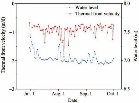
Figure 9 Thermal front velocity and water level changes at S1 from July to September in 2015

5 Conclusions

This study demonstrated the potential of heat tracing methods for studying the interaction of SW-GW across a streambed in permafrost regions of the northern Tibetan Plateau. The 1-D HTE analytical heat tracing in the observation sites revealed increasing SW-GW interaction induced by active layer thawing. The SW-GW interaction tended to increase with time in the areas with permafrost, occurring in association with the thickening of the active layer.As the active layer thawing and groundwater table become deeper beneath the stream later in thaw periods,reaches with water loss in permafrost areas may become more disconnected. The results from this study indicate that the heat tracing method can offer strong evidence for the increasing SW-GW interaction induced by permafrost thaw.

Although no up-welling groundwater in the observation area, the FO-DTS monitoring, when combined with 1-D HTE analytical analysis, is proved to be a useful indicator for the identification of temporal and spatial patterns of SW-GW interaction. By comparing the heat trace from the 1-D HTE analysis with the temperature anomalies observed by the FO-DTS, this study offers a validated strategy for optimizing the experimental design in a permafrost region with limited information of streambed structure and physical and thermal properties.

This approach has been validated for the SW-GW interaction between summer streams in permafrost regions and the active layer in thaw periods. Future work should focus on the applicability of the present approach in other seasons and adapting it for complicated streambed environments in permafrost regions,including areas with or without permafrost and talik zones.

Acknowledgments:

This work was supported by the National Natural Science Foundation of China (41690141, 41671067), the second Tibetan Plateau Scientific Expedition and Research Program (STEP) (2019QZKK0605), the Fundamental Research Funds for Central Universities(lzujbky-2019-40), CAS "Light of West China" and the State Key Laboratory of Cryospheric Science,CAS(SKLCS-ZZ-2020).