Method for denoising and reconstructing radar HRRP using modified sparse auto-encoder

Chen GUO, Haipeng WANG, Tao JIAN, Congan XU, Shun SUN

Information Fusion Institution, Naval Aviation University, Yantai 264001, China

KEYWORDS High resolution range profile;Intrinsic dimension;Modified sparse autoencoder;Signal denoise;Signal sparse reconstruction

Abstract A high resolution range profile (HRRP) is a summation vector of the sub-echoes of the target scattering points acquired by a wide-band radar. Generally, HRRPs obtained in a noncooperative complex electromagnetic environment are contaminated by strong noise. Effective pre-processing of the HRRP data can greatly improve the accuracy of target recognition. In this paper, a denoising and reconstruction method for HRRP is proposed based on a Modified Sparse Auto-Encoder, which is a representative non-linear model. To better reconstruct the HRRP, a sparse constraint is added to the proposed model and the sparse coefficient is calculated based on the intrinsic dimension of HRRP.The denoising of the HRRP is performed by adding random noise to the input HRRP data during the training process and fine-tuning the weight matrix through singular-value decomposition. The results of simulations showed that the proposed method can both reconstruct the signal with fidelity and suppress noise effectively, significantly outperforming other methods, especially in low Signal-to-Noise Ratio conditions.

1. Introduction

The High Resolution Range Profile (HRRP) is a onedimensional projection in the radar observation direction obtained by a wide-band radar(whose resolution is far smaller than the target size). The HRRP contains abundant information regarding the scattering points of the target, such as the Radar Cross-Section (RCS), the distribution of scattering points along the direction of arrival, and the structure and intensity of the scattering center, etc.1Compared with the two-dimensional resolution range profile, the HRRP is significantly easier to obtain, process and store. Therefore, it has become a topic of active research in the field of radar automatic target recognition using radar.

In practice, the data used for training and testing are often obtained under non-cooperative complex electro-magnetic environment. It is difficult to obtain a high Signal-to-Noise Ratio (SNR) HRRP especially when the target is located far from the radar. The weak scattering points of the target are prone to being submerged in the noise under low SNR conditions, resulting in a significant reduction in the target recognition accuracy. Therefore, it is necessary to develop processing methods for HRRP under low SNR conditions. Currently,there are three primary methods available for processing noisy HRRPs: HRRP reconstruction and denoising,2,3noise-robust feature extraction of the HRRP4-9and establishing noiserobust statistical models of the HRRP.10,11In this study,we will focus on the first one,that is,the denoising and reconstruction of noisy HRRP.

In recent years,there has been extensive research in this field.For instance,a denoising method for HRRP based on Singular Value Decomposition (SVD) was proposed in Ref.2. This method splits the test data into the signal subspace and the noise value subspace based on the concept of subspaces and suppresses the noise by performing SVD on the Hankel-form matrix of the test data.Data reconstruction is performed by setting the singular value to be less than a certain threshold to zero. In Ref.12,a signal reconstruction method was proposed based on the ConVeX optimization algorithm (CVX). In order to find the best approximation of the signal based on prior knowledge of the noise,this method converts the non-convex problem into a convex one,which is easier to solve.Signal denoising methods based on Bayesian Sparse Decomposition(BSD)have also been proposed.13-16In this method, the reconstructed signals is obtained by posteriori estimating the expansion coefficient and noise power using the Bayesian formula based on the assumption that the priori distribution of the signal and noise is known. Noise suppression methods based on Orthogonal Matching Pursuit(OMP)have also been developed.3,17,18These methods reconstruct the signal by selecting a local optimal solution at each iteration step.When the norm of the error between the reconstructed signal and the noisy signal is smaller than the noise power,the iterations are stopped,yielding the expansion coefficient. The advantage of these methods is that a single HRRP can be denoised and reconstructed. However, prior knowledge of the noise is required and the denoising performance is poor under low SNR conditions.Therefore,methods based on K-SVD were proposed to solve the problem of denoising under low SNR conditions.19-22Unlike the methods based on OMP,the K-SVD algorithm is used to update the dictionary atoms based on the training data after each OMP operation.Therefore,a certain amount of training data is required.

At present, the conventional methods employed for signal reconstruction and noise reduction are sparse representation methods based on dictionary learning, wherein high dimensional input data are represented as a linear combination of weighted dictionary atoms.The performance of the sparse representations depends on factors such as the SNR conditions,over-complete dictionary atoms, and sparse coefficient among others.Therefore,there are two obvious shortcomings of these methods: (A) prior knowledge of the noise distribution is required and(B)the denoising and reconstruction performance of these methods is poor under low SNR conditions.

With the above problems in mind, a denoising and reconstruction method for HRRPs is proposed based on a Modified Sparse Auto-Encoder (MSAE). The auto-encoder is an effective model for reconstructing the signals. To improve the robustness of the model, random noise is added to the input signal during every epoch.In order to present the signals more sparsely, the sparse constraint of the objective function is designed based on both the average and the variance of the activation values of the neurons in the hidden layer. Furthermore, the sparse coefficient is determined by the intrinsic dimension of the HRRP dataset instead of through experiments. To solve the problem of insufficient training data,SVD is performed on the weight matrix of the trained model to further improve the denoising performance. Experimental results confirmed that the reconstruction and denoising performance of this method under low SNR conditions is much better than those of the other available approaches.

The rest of this paper is structured as follows.In Section 2,the HRRP data and autoencoder are introduced.In Section 3,the MSAE is described comprehensively in three parts:(A)the objective function of the MSAE is described, (B) the intrinsic dimension of the HRRP dataset is estimated for calculating the sparsity parameter and (C) the physical meaning of the weight matrix is explained and the method for modifying the weight matrix is described. In Section 4, the HRRP dataset and the simulation procedures are described.Next,the simulation results are presented and analyzed in Section 5.Lastly,the conclusions of the study are summarized in Section 6.

2. Description of HRRP data and auto-encoder

2.1. Description of HRRP

The HRRP is the amplitude of the coherent summations of the complex time returns from the target scatterers in each range cell.1The radar signature of each radar range cell can be considered to be the superposition of the radar echoes from all the scatterers within the corresponding range cell. When the resolution of the radar is much smaller than the target size,the target occupies multiple radar range cells. Usually, the model of the scatterers is adopted to describe the HRRP of the target,and the mth complex returned echo in the nth range cell xn（m ） can be approximated as

where Indenotes the number of target scatterers in nth the range cell, Rn,i（m ） denotes the radial distance between the radar and the i th scatterer in the m th sampled echo, and σn,iand θn,irepresent the amplitude and initial phase of the i th echo. The nth HRRP can be expressed as

where D is the dimension of the HRRP data and ｜（·）｜represents the modulo operation.

The HRRP data used in this study was generated by using the electromagnetic simulation software CST MICROWAVE STUDIO®and the results for one single HRRP are presented in Fig.1.As can be seen from Fig.1(a),the red part of the ship represents its scattering surface in the direction of the incident angle of the radar. For ship targets, the strong scatterers are mainly concentrated on the hull and the bulges on the deck(marked with circles in Fig. 1 (a)). It can be seen from Fig. 1 (b) that the HRRP of the target is sparse; however,the noise is not. Therefore, we can sparsely represent the HRRP data to achieve noise suppression.

2.2. Description of auto-encoder

According to the universal representation theorem proposed in Ref. 23, any vector can be represented by a non-linear function. The related formula is

where, ‖·‖2represents the Euclidean norm, M is a random Gaussian matrix and f:R →R is a semi-truncated linear function, which satisfies the condition f（0 ）=0(0 ＜f （x ）≤x,∀x ＞0), and 0 ≥f （x ）≥x （∀ x ＜0）. The Rectified Liner Uints (ReLU) and the sigmoid function are examples of such a function.A （·）can be a linear or non-linear function such as the sigmoid or identity function.

Fig. 1 Scattering surface of ship and its corresponding simulated RCS at incident angle of 45°.

Non-linear representations often contain more target information than linear ones.As mentioned previously,in this paper,a nonlinear sparse representation method based on an autoencoder is proposed.This method can denoise and reconstruct noisy HRRP data well.At the same time,this method exhibits good robustness.The basic structure and function of the autoencoder are shown in Fig.2 and then described in the text that follows.

An auto-encoder consists of three parts: an input layer, a hidden layer, and an output layer.24-26The auto-encoder model shown in Fig. 2 has only one hidden layer. The input layer has the same number of neurons as that of the output layer. The mapping from the input layer to the hidden layer is called encoding. Correspondingly, the mapping from the hidden layer to the output layer is called decoding.

Encoding: The input vector is mapped to the hidden layer.The process can be described by the following formula:

Decoding: The h ∈[0,1 ]Kof the hidden layer is mapped to the output layer to reconstruct the required vector. This process can be described by the following formula?

where, ^x is the reconstruction vector,WTand bTrepresent the transposition of the weight matrix W and bias b during the encoding process, respectively and g （·） is a mapping function,which adopts a sigmoid function in this study.

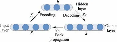
Fig. 2 Auto-encoder with single hidden layer.

3. Description of MSAE model

The design of the model proposed in this paper draws on the conventional sparse representation method and consists of the following three primary parts: an objective function for sparse reconstruction, a method for determining the sparse coefficient and the modification of the weight matrix.

3.1. Objective function of MSAE

The core idea of dictionary learning is to sparsely represent the signal by using dictionary atoms. This process can be expressed as

where,～x ∈RNis noisy data consisting of the signal x ∈RNand noise n ∈RN, ^x ∈RNis the reconstructed signal,D= ｛dk,k=1,2,···,K｝ is the dictionary, dk∈RNis the k th atom in the dictionary, and ξ= ｛ξk,k=1,2,···,N｝ is the expansion coefficient of the signal. Because of the overcompleteness of the dictionary D, ξ is not unique. Therefore,constraints are needed to determine the expansion coefficient as

It can be seen from Eq. (8) that, in order to achieve noise reduction and sparse reconstruction, the method introduces two distinct constraints.First,the number of dictionary atoms is constrained.Second,the norm of the reconstruction error is smaller than the noise power.We apply the same sparse reconstruction ideas to auto-encoder model to obtain the MSAE.The structure of the proposed model is shown in Fig. 3.

The function of the auto-encoder is mainly embodied in the objective function.In order to realize the sparse representation of the HRRP, the objective function of MSAE is

Here, the first part of the function is called the error term which is designed to minimize the error between the reconstruction ^x and the original vector x,and L （·）is the loss function.Because a Stochastic Gradient Descent(SGD)is adopted

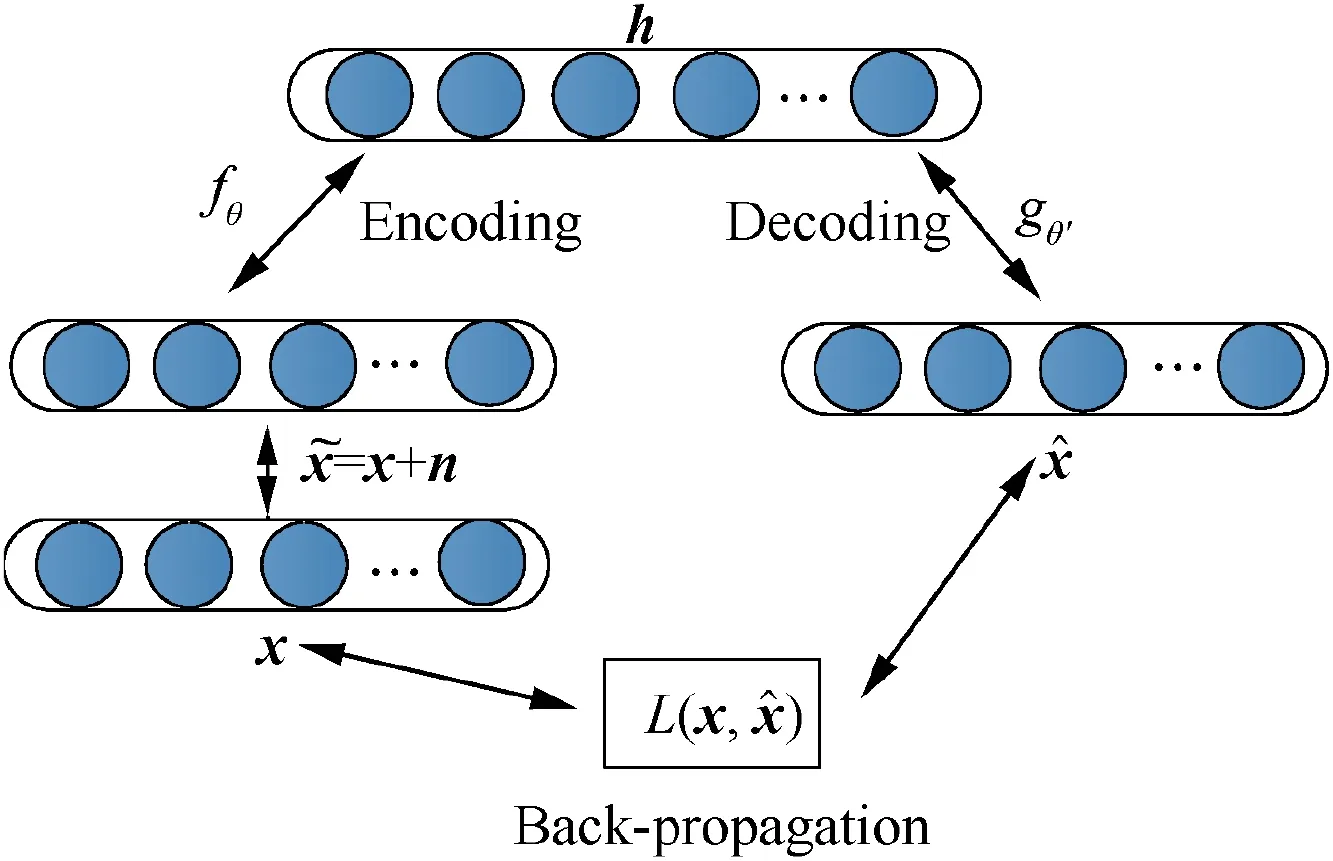
Fig. 3 Schematic diagram of proposed model.

where, m is the number of training samples in min-batch.

The second part of the function is called the regularization term, which is adopted to prevent overfitting. The hyper parameter λ controls the weight of the regularization term.The expression for Ωwis

where,D is the dimension of the input data and H is the number of the neurons in the hidden layer. Ωwpenalizes the larger elements of the weight matrix.

The third part of the function is called the sparsity term,which is designed to make sparse the hidden representation,here, β is a hyper parameter, which controls the weight of the sparsity term. The function for the sparsity term is

3.2. Setting of sparse coefficients and number of hidden layer neurons

In order to fully represent the input vector, the dictionary for sparse representation must be over-complete. Sparse reconstruction is achieved by constraining the number of non-zero values in the expansion coefficients. Generally, an autoencoder is used to extract the features.Therefore, H is smaller than D. Learning from the case of sparse representation using dictionary learning,H should be larger than D,and the sparse constraints should be exerted put on the activation of the neurons in the hidden layers.

In this section, a method for estimating the sparse coefficients is proposed based on the intrinsic dimension. The intrinsic dimension refers to the smallest dimension that can represent the HRRP.27The sparse coefficients of the MSAE are determined both by the intrinsic dimension of the HRRP dataset and the number of neurons in the hidden layer. Since the HRRP dataset was simulated by the software CST in the full angle domain, a global intrinsic dimension estimation method is proposed to maintain the topological structure of the dataset. Simultaneously, the relationship between the local neighboring data and the distance constraints of non-adjacent data is considered, In other words, the neighboring data are expected to be closer and the non-adjacent data are expected to be lie farther away.The algorithm for calculating the intrinsic dimension is given as below.The HRRPs for different angle domains are very different.The relationship between xi∉Ωjand xj∉Ωiis non-linear.It is not appropriate to represent the weight between xi∉Ωjand xj∉Ωiby the Euclidean distance. However, the HRRP data can be considered continuous in the angle domain because of similarity between the adjacent angles. Therefore, the Isometric feature mapping(Isomap)algorithm is adopted to compute the global weight matrix G.29,30Dijis calculated for the following steps

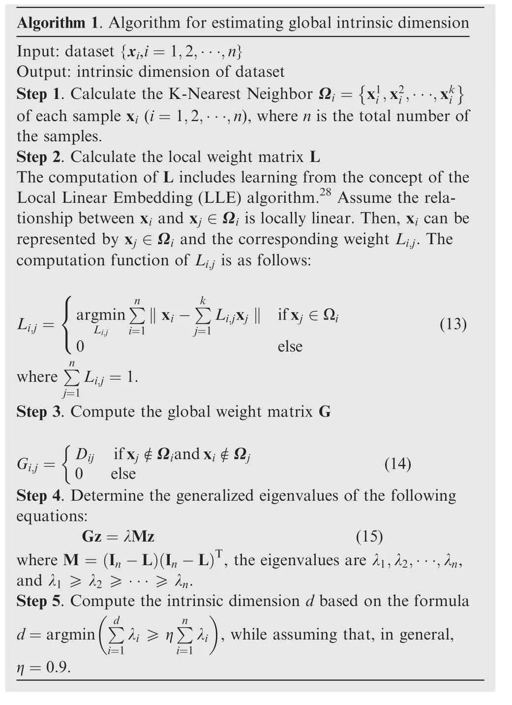
Algorithm 1. Algorithm for estimating global intrinsic dimension Input: dataset {xi,i=1,2,···,n}Output: intrinsic dimension of dataset Step 1. Calculate the K-Nearest Neighbor Ωi = x1i,x2i,···,xki■■of each sample xi (i=1,2,···,n), where n is the total number of the samples.Step 2. Calculate the local weight matrix L The computation of L includes learning from the concept of the Local Linear Embedding (LLE) algorithm.28 Assume the relationship between xi and xj ∈Ωi is locally linear. Then, xi can be represented by xj ∈Ωi and the corresponding weight Li,j. The computation function of Li,j is as follows:■■ ■Li,j = argmin ∑n ‖xi-∑k Li,jxj ‖ if xj ∈Ωi 0 else(13)where ∑n Li,j i=1 j=1 Li,j =1.Step 3. Compute the global weight matrix G Gi,j = Dij if xj ∉Ωiand xi ∉Ωj 0 else j=1&(14)Step 4. Determine the generalized eigenvalues of the following equations:Gz=λMz (15)where M = In-L In-LT, the eigenvalues are λ1,λ2,···,λn,and λ1 ≥λ2 ≥···≥λn.Step 5. Compute the intrinsic dimension d based on the formula d=argmin ∑d λi ≥η ∑n , while assuming that, in general,η=0.9.λi i=1 i=1

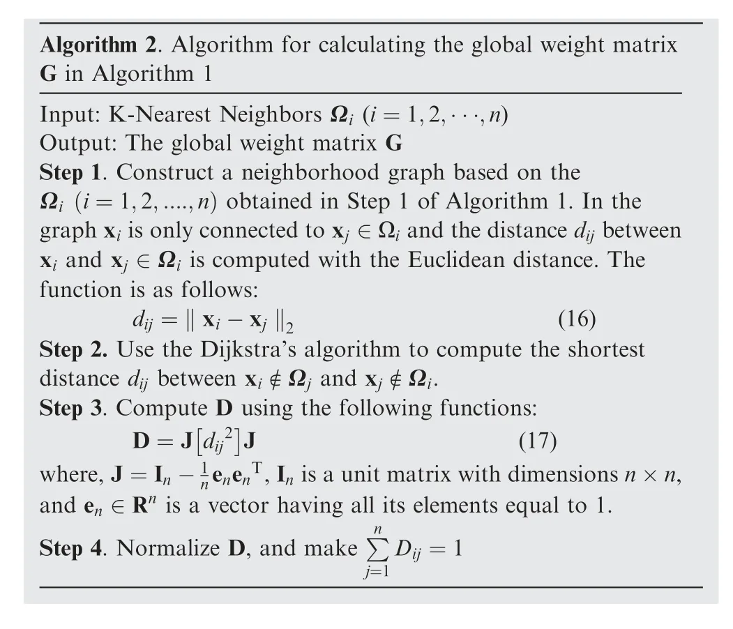
Algorithm 2. Algorithm for calculating the global weight matrix G in Algorithm 1 Input: K-Nearest Neighbors Ωi (i=1,2,···,n)Output: The global weight matrix G Step 1. Construct a neighborhood graph based on the Ωi i=1,2,....,n） obtained in Step 1 of Algorithm 1. In the graph xi is only connected to xj ∈Ωi and the distance dij between xi and xj ∈Ωi is computed with the Euclidean distance. The function is as follows:dij =‖xi-xj ‖2 (16)Step 2. Use the Dijkstra’s algorithm to compute the shortest distance dij between xi ∉Ωj and xj ∉Ωi.Step 3. Compute D using the following functions:D=J dij2■ ■J (17)where,J=In-（1n enenT,In is a unit matrix with dimensions n×n,and en ∈Rn is a vector having all its elements equal to 1.Step 4. Normalize D, and make ∑n Dij =1 j=1

3.3. Modification of weight matrix

The SGD method is adopted to update the model weight matrix during training. Theoretically, the loss function should approach zero after training. However, in practical applications, owing to factors such as insufficient training data, the loss function can only approach a relatively small value.Hence, the HRRP reconstructed using MSAE still contains noise information. In order to better denoise and reconstruct the data, we need to further process the weight matrix W.The connecting lines in Fig. 4 represent the elements of the weight matrix W.

As shown in Fig.4,each connecting line corresponds to an element of the weight matrix. The initial weight obeys the Gaussian zero mean distribution. With the output ^x continuously approaching x, the weights corresponding to the input x increase, while those corresponding to the noise n decrease continuously during the training period.Together,the weights corresponding to the noise are regarded as the noise weight.The noise can be suppressed more effectively after reducing the corresponding weight. Therefore, the SVD algorithm is applied to the weight matrix to better suppress the noise.31The weight matrix W can be decomposed as follows:

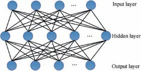
Fig. 4 Schematic of weight matrix.

where W is the weight matrix of the MSAE with dimension K×D, U is an orthogonal matrix with dimension K×K, V is an orthogonal matrix with dimension D×D, Λ is a matrix with dimensions K×D, Λ=diag（σ1,σ2,···,σD,0,···,0）,and σ1≥σ2≥...≥σ. Further, uiis the i th column of U and viis the i th column of V. W can also be expressed as

4. Dataset and experimental procedure

4.1. Dataset

It is difficult to establish a target HRRP dataset through measurements because of the non-cooperative properties of the targets. Therefore, the software CST was employed to simulate the HRRP data. The 1:1 target model shown in Fig. 5 was established using the 3-dimensional software Solidworks and imported into CST. Several factors were considered before the simulation:

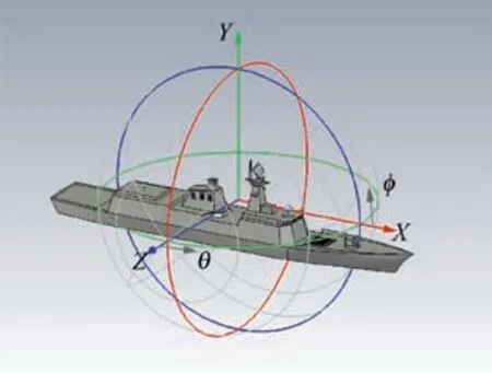
Fig. 5 Ship model.

(1) To begin with,it was assumed that the target is a type of super-large electric target. During the simulation, the CST developed an extremely fine mesh model of the ship,which calls for high performance of the computers.Next, the HRRPs between the adjacent angles were assumed to be similar to each other.Therefore,we could choose a large angle step.

(2) The ship model used in this study was assumed to be symmetrical, hence, only half of the target had to be simulated.

Combining the above factors, the CST simulation parameters were set as follows: azimuth angle of -90°to 90°, pitch angle of 0°,and angle step of 1°.For the radar, the center frequency was 10 GHz, bandwidth was 100 MHz, the polarization method was V, and the number of frequency sampling points was 256.

Finally, the simulation yielded 181 azimuthal angle HRRP data for seven ship targets.

The target HRRP was obtained by converting the RCS of the range cell simulated with CST using radar equation. Since the simulation background was simple, the HRRP obtained from the simulation could be regarded as noise-free data.However, the HRRP simulated with CST was insufficient for training the proposed model. Therefore, the dataset was expanded by interception. The dimension of the data obtained from CST was 1024. Since the model was placed at the origin of the coordinate axis during the simulation,the points reflecting the characteristics of the model were distributed symmetrically with the center point being 512, hence,we performed the interception with 512 as the center point,20 as the step size and 512 as the length of the interception window, and then translated to the left and right sides five times. Using this method, the dataset could be expanded by a factor of 10.

In order to simulate the actual scene, the noise was superimposed on the raw HRRP.Usually,the SNR of training data is high and set to 20 dB.In order to test the recognition performance of the target HRRP under different SNR conditions,the SNR of the test data was set as 0, 5, 10 and 15 dB. The SNR is defined as the ratio of the signal power to the noise power:

where, Psand Pnrepresent the power of the signal and noise respectively. The HRRP dataset for different SNR values could be obtained by adding noise to the noise free HRRP,the noise power σi2was calculated according to Eq. (21).The number of trainings and test data obtained by this method were both 7×181×10=12670. It is worth noting that the training and test dataset did not overlap.

4.2. Experimental procedure

MATLAB2016b was used for data processing and the algorithmic simulations. The proposed models can be obtained by the following steps:

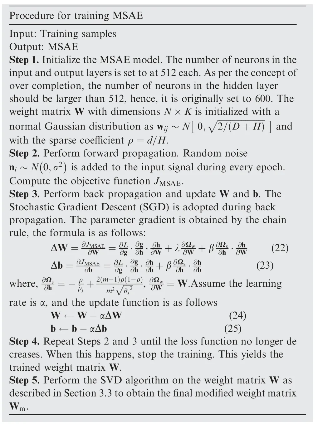
Procedure for training MSAE Input: Training samples Output: MSAE Step 1.Initialize the MSAE model.The number of neurons in the input and output layers is set to at 512 each.As per the concept of over completion, the number of neurons in the hidden layer should be larger than 512, hence, it is originally set to 600. The weight matrix W with dimensions N×K is initialized with a normal Gaussian distribution as wij ～N 0,■■■■■■■■■■■■■■■■■■■■2/ D+H■■and with the sparse coeきcient ρ=d/H.Step 2. Perform forward propagation. Random noise ni ～N 0,σ2■ ■is added to the input signal during every epoch.Compute the objective function JMSAE.Step 3. Perform back propagation and update W and b. The Stochastic Gradient Descent (SGD) is adopted during back propagation. The parameter gradient is obtained by the chain rule, the formula is as follows:ΔW=■∂JMSAE∂W =∂L∂g·∂g∂h·∂h∂W (22)Δb=∂W+λ∂Ωw ∂W +β∂Ωs∂h ·∂h∂JMSAE∂b =∂L∂g·∂g∂h·∂h∂b (23)where,∂b+β∂Ωs∂h ·∂h∂Ωs ∂W =W.Assume the learning rate is α, and the update function is as follows W ←W-αΔW (24)b ←b-αΔb (25)Step 4. Repeat Steps 2 and 3 until the loss function no longer de creases. When this happens, stop the training. This yields the trained weight matrix W.Step 5. Perform the SVD algorithm on the weight matrix W as described in Section 3.3 to obtain the final modified weight matrix Wm.∂h =-ρ^ρj+2 m-1ρ 1-ρm2 ■■■■■ ,∂Ωw^σj2

5. Simulation results and analysis

In order to analyze the reconstruction performance of the algorithms quantitatively, we define the Mean Square Error(MSE)as the evaluation metric.The smaller the MSE,the better the reconstruction performance was:

where xirepresents the i th test data, ^xirepresents the reconstructed data of xiand ntrepresents the number of test data.All the simulations were performed 100 times to obtain the average result as the effective MSE.

5.1. Effect of number of hidden layers on reconstruction performance

From simulation Step 1 in Section 4.2,we know that D is 512.Irrespective of whether H is larger or smaller than D, ^ρ will be approximately equal to ρ at the end of the training process.In order to elucidate the effect of H on signal reconstruction, H was taken to be 100, 200, 300, 400, 500, 600, 700 and 800.

As stated in Section 3.2, the intrinsic dimension of the HRRP is 180. The sparsity parameter can be obtained from ρ=180/H.Because 100 ＜180,when H=100,we set the corresponding sparsity term coefficient as β=0.The result of the simulation is shown in Fig. 6.

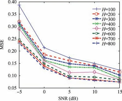
Fig. 6 MSE for reconstruction under different SNR conditions with different number of neurons in hidden layer.

As shown in Fig. 6, the reconstruction MSE of the model for the different H values is generally small, and gradually decreases with the increase of H under high SNR situations.The reconstruction MSE for the models with different H values still decreases gradually with the increase in H. However,the reconstruction performance of the model with H ＞D is significantly better than that of the model with H ＜D in low SNR situations. On the other hand, when H ＞D, the reconstruction MSE of the model increases slightly with the increase of H.This is because the model with more hidden neurons can better represent the data,but when H is too large,the training process is prone to over-fitting, which results in poor reconstruction performance for the test samples. Therefore, we chose to keep H slightly larger than D and set it to 600. The corresponding sparsity parameter ρ was 0.3.

5.2. Selection of hyper-parameters There are three hyper-parameters related to the MSAE model,namely,learning rate α,regularization coefficient λ,and sparse coefficient β.These parameters were selected through trial and error.

(1) Selection of learning rate α

The learning rate determines the convergence performance of the model.A high learning rate will lead to significant oscillations in the loss, while a small one will lead to slow convergence.The initial value of the learning rate does not need to be precise.

Assume that the initial learning rate is Δ and that the number of training epochs is 100. If the objective function oscillates, it means that the learning rate is too large, and its initial value rate can be halved to Δ/2.Continue the above iteration until the objective function starts to converge. If the objective function converges slowly, double the initial value of the learning rate until the objective function oscillates,and select the first previous value as the initial learning rate.During the training process, when the average change in the objective function within 10 epochs is less than 10-5, halve the learning rate, and when the average change is less than 10-9, stop the training process. The convergence speed of this method was approximately five times faster than the invariant learning rate. The initial learning rate was set to 0.02. As shown in Fig. 7, a suitable learning rate ensures that the loss curve (representing the objective function) of the model decreases faster and is more stable.

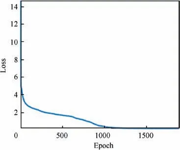
Fig. 7 Training loss curve.

(2) Selection of regularization coefficient λ and sparsity coefficient β

The role of the regularization term is to prevent overfitting.A small λ leads to overfitting,while a large one leads to a large convergence value of the objective function.Usually,the initial regularization coefficient is set to be a small number such as 0.001,and the order of magnitude is then determined by zooming the initial value in or out 10 times until the best performance is achieved. The order of λ was set to 10-5after the simulation.Further,β controls the weight of the sparsity term,usually taken to be an integer, Thus, we assumed β ∈[1,5 ],λ ∈[ 1,9]×10-5. Then, a grid search method was used for the cross validation of λ and β.32The values chosen finally were λ=6×10-5and β=2.

5.3. Effects of number of hidden layers on reconstruction performance

Next, the performances of four methods were compared with that of MSAE in order to evaluate the latter. These were denoising methods based on CVX, OMP, BSD, and K-SVD.MSE was used as the metric to measure the reconstruction performances, as shown in Table 1.

It can be seen from Table 1 that, when SNR=15, the reconstruction performance of MSAE was inferior to those of the other four methods. When SNR=10, however, the reconstruction performance of MSAE was slightly better than those of the other four. On the other hand, when SNR=5,the MSE of MSAE was markedly lower than those of the others algorithms. Finally, when SNR=0, the MSE of MSAE was even lower. Further, the MSE values for MSAE for SNR values of 5, 10, and 15 were similar, indicating that MSAE is highly robust.

In order to further elucidate the reconstruction and noise reduction performance of MSAE, the results for OMP and K-SVD were analyzed in depth. The simulation results forthe three algorithms under different SNR conditions are shown in Figs. 8 and 9.

Table 1 MSE for different methods under different SNR conditions.

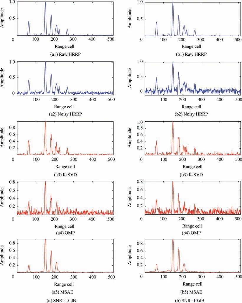
Fig. 8 Denoising and reconstruction results of dictionary learning method and proposed method under high SNR conditions.

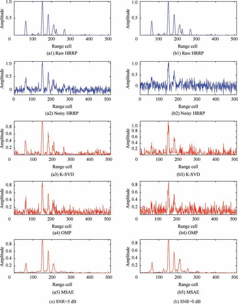
Fig. 9 Denoising and reconstruction results of dictionary learning methods and proposed method under low SNR conditions.

It can be seen from Fig.8 that the signal could be denoised and reconstructed effectively by both MSAE and the dictionary learning methods under high SNR conditions.The methods based on dictionary learning even exhibited better reconstruction performances.From the figures labeled with OMP and K-SVD in Figs. 8 (a) and (b), it can be seen from that the strong scattering units as well as the weak scattering units were well reconstructed by both OMP and K-SVD. In terms of denoising, OMP reconstructed a small amount of the noise and exhibited good denoising performance overall.The K-SVD algorithm smoothened the noise and showed better noise suppression performance than that of OMP. From the figures labeled with MSAE in Figs. 8 (a) and (b), it can be seen that MSAE exhibited good reconstruction performance for the strong scattering units but showed poor reconstruction performance for the weak ones. The weaker the scattering units were,the worse its reconstruction performance was.Although MSAE showed a better denoising performance,the MSE of MSAE was larger than those of the other two methods because of its poor reconstruction performance for the weak scattering units.

Further, it can be seen from Fig. 9 that, the reconstruction performance of MSAE was obviously better than those of OMP and K-SVD under the low SNR conditions. The reconstruction performance of OMP and K-SVD reduced sharply with a decrease in the SNR. As is evident from the figures labeled with OMP and K-SVD in Figs. 9 (a) and (b), there were large deviations in the reconstructions of the strong scattering units and the weak scattering units in the case of OMP,and many strong noise points were also reconstructed.Although reducing the sparse coefficient helped suppress the noise better, it also resulted in the incorrect reconstruction of the signal. It is difficult to simultaneously improve the signal reconstruction and denoising performance. Compared with OMP, K-SVD showed better reconstruction performance in terms of both the strong scattering units and the weak ones,however, it showed poorer denoising performance. Although the overall noise was reduced, it still existed in each unit and had a large effect on weak scattering units. Further, it can be seen from the figures labeled with MSAE in Figs. 9 (a) and(b) that, in these conditions too, MSAE showed good reconstruction performance for the strong scattering units but relatively poor reconstruction for the weak ones. In terms of denoising, the proposed method performed very well. Compared with OMP, MSAE did not reconstruct the noise corresponding to the target scatters. Further, compared with KSVD, MSAE showed very good denoising performance for each unit. This was because, as also stated above, non-linear representations often contain more target information than linear ones. This was the reason MSAE performed better that the linear algorithms, exhibiting better representation performance and resulting in a smaller loss in information.

Since the strong scattering units contain most of the target information, it is more important that they are reconstructed with accuracy.Therefore,MSAE can be considered a good signal reconstruction method.Further,MSAE showed better performance with respect to both signal reconstruction and denoising than other methods, especially under low SNR conditions.Moreover,with a decrease in the SNR,the reconstruction and denoising performance of MSAE remained at a high level.

5.4. Effects of number of hidden layers on reconstruction performance

Finally, to better highlight the effectiveness of the proposed algorithm, the target recognition accuracy of the denoised HRRP was simulated.In the simulation,two typical classifiers were selected for target recognition:these were an Linear Support Vector Machine(LSVM),which represented linear classifiers, and a Convolutional Neural Network (CNN), which represented nonlinear classifier; the structure of the CNN was the same as that of the classical CNN adopted in.33The simulation results are listed in Table 2,which shows the recognition accuracy of mapping of the classifiers, the denoising algorithm used,and the SNR;RA stands for recognition algorithm, DA stands for denoising algorithm, ACC denotes the recognition accuracy, and NONE means that the HRRP was not subjected to denoising.

It can be seen from Table 2 that, the LSVM was more sensitive to noise. Therefore, the denoising performance had a greater influence on its recognition accuracy. When SNR=15 dB, the accuracy of MSAE was slightly lower than those of the other two DAs, whereas, with a decrease in the SNR, the advantage of MSAE gradually emerges. In particular, for SNR=0 dB, the accuracy was of MSAE was significantly better than those of the other algorithms.In conclusion, from the perspective of recognition accuracy,the denoising performance of MSAE was better than those of the other two DAs especially under the low SNR conditions.

6. Conclusions

(1) An effective denoising and reconstruction method for HRRPs was proposed based on MSAE.

(2) The proposed method shows good denoising and reconstruction performance especially under low SNR conditions. With a decrease in the SNR, the performance of the proposed method remains high, indicating that it has high robustness.

(3) Another advantage of the proposed model is that it requires no prior knowledge of the noise.

(4) The proposed method also has a few deficiencies. To begin with,it requires a certain amount of data for training. Thus, it cannot handle noise reduction problems in the case of single data. Secondly, the proposed method exhibits poor performance during the reconstruction of weak scatters.

Acknowledgements

This study was co-supported by the National Natural Science Foundation of China (Nos. 61671463, 61471379, 61790551 and 61102166).

Table 2 Recognition accuracy for denoised HRRP.