A global solution for robust parameter design of aeronautical electrical apparatus based oninteractions analysis and polynomial fitting

Jie DENG, Xuerong YE,*, Jinhu XUE, Guofu ZHAI

a School of Electrical Engineering and Automation, Harbin Institute of Technology, Harbin 150001, China

b Department of Research and Development, Wuxi Newhongtai Electrical Technology Co., Wuxi 214174, China

KEYWORDS Aeronautical electrical apparatus;Global optimization;Interactions analysis;Polynomial fitting;Robust parameter design

Abstract Robust Parameter Design(RPD)has been widely applied for improving quality and reliability of products. One of the key drawbacks of applying RPD using Taguchi method is that the stable factors may not be independent of the adjustment factors,resulting in unsatisfactory design.Moreover,the Taguchi method cannot guarantee global optimality since the levels set in the experiment are usually discrete to ensure orthogonal design. In this paper,robust solutions of the stable factors are obtained via a nonlinear model based on polynomial fitting;while the adjustment factors are obtained via interactions analysis so that they are independent of the stable factors. In particular, the values of the adjustment factors are determined by output offset compensation so as to achieve robustness of the design scheme. An example on the design of an aeronautical electrical apparatus is presented to illustrate the procedure. The results show that the proposed method can take full advantage of the nonlinearity in the response and achieve the desired outcome.

1. Introduction

Uncertainties in the manufacturing process is the fundamental reason of output variation from the designed values.1-3It directly affects the consistency and reliability of batch products,4,5especially for the aeronautical electrical apparatus containing a great many technique processes during the manufacture.6In order to improve the robustness through the parameter optimization, Taguchi et al proposed the basic idea of quality loss and established the Robust Parameter Design(RPD)method.7,8The Signal to Noise ratio(SN ratio)is firstly introduced to describe the impact of uncertainty factors on the output characteristics.9-11Moreover,the nonlinearity among the input parameters and output characteristics is utilized to improve the robustness under the conditions of‘no change of cost’.12-14The RPD method has been proved successfully in many fields.15-18For instance, Wang Z.F. and Wang H.19used Taguchi method to obtain the optimum factors for the lowest deflection and largest value of SNR of inflatable wing.Tiryaki et al.20used Taguchi method to determine the optimal settings of process parameters and obtained the lower surface roughness values in wood machining process.

The fundamental principles of the Taguchi method are widely recognized.21-23However, there are still many arguments focusing on the techniques of experimental design.24,25Leon et al.26pointed out that there are many real life problems in which the SN ratio is not independent of the output mean,and its use can lead to design parameter settings being far from optimal. In response to this issue, Box27put forward PerMIA(Performance Measure Independent of Adjustment) in which an appropriate transformation Y=h(y) is made so that the standard deviation σYis independent of the mean μY.

Although the PerMIA has been proven to be theoretically possible in solving RPD problems,28the appropriate transformation Y=h(y) may not be easy to identify in practical. In view of this,the interactions analysis is proposed in this paper so that appropriate adjustment factors which are independent of stable factors can be identified.Unlike the PerMIA method which directly determines the optimal values of the parameters through the transformation process,our proposed method first identifies the factor types and then determines the optimal values.

Another drawback of the Taguchi method is that, even if SN ratio is statistically independent of the adjustment factors,the results are not necessarily optimal.29This is because of discontinuity and the large difference of the levels in orthogonal table.The optimization scheme may not result in true optimal solution within the scope of parameter variation.30Therefore,effective global robust optimization has also been a hot topic in the field of robust design.31-33It is expected that the use of the surrogate model is able to overcome the difficulty resulting from the computational expense of the uncertainty analysis in the robust design, so as to improve the accuracy and efficiency of global optimization.34-36For example, Rehman and Langelaar37proposed a globally robust design by searching for the best worst-case cost,which involves model building using Kriging method.Gan et al.38combine numerical simulation method and RBF surrogate model to build the deterministic optimization process of robust design for the conformal expansion nozzle of flying wing unmanned aerial vehicle.

However,in order to ensure the accuracy of the model containing all the factors, a large number of samples still need to be collected. To address this shortcoming, we propose using nonlinear polynomial for modeling only the stable factors. In this way, the optimal robust solution can be obtained via the global searching algorithm similar to the Response Surface Methodology (RSM).

In this paper, we proposed an improved RPD method that combines interactions analysis, polynomial fitting and global optimization.The interactions analysis is used for factors classification so that appropriate stable factors which are independent of adjustment factors can be obtained. At the same time,it can effectively reduce the number of factors when building the nonlinear function model, so as to increase the modeling accuracy. Then polynomial fitting is adopted to establish the functional relationship among the factors and the output characteristics. Finally, the stable factor values are determined for robustness by the global optimization,and the adjustment factor values are calculated for the offset compensation of output.

The remainder of the paper is organized as follows. Section 2 gives a brief description of the design process of the improved RPD method. Subsequently, theoretical models of significance analysis, interactions analysis, and the establishment of optimization functions are presented in Section 3.Section 4 illustrates the effectiveness of the proposed method via an RPD optimization of an aeronautical electrical apparatus.Finally, conclusions are given in Section 5.

2. Procedure of the proposed RPD method

A three-step procedure containing the determination of two types of design parameters (d, a)⊂θ is proposed here, where d represents stable factors, a represents adjustment factors and θ represents the design parameters.

Step 1.Find the setting d=d*that maximizes the SN ratio(Same as the Taguchi method).

Step 2.Find the adjustment parameter a via the interactions analysis (Additional step).

Step 3. Adjust a to a* to compensate the offset while d is fixed at d* (Same as the Taguchi method).

The procedure of the improved RPD method is shown in Fig. 1. Firstly, the appropriate orthogonal table is selected by the number of factors and their levels. An orthogonal experiment is designed with the experimental factors in the inner array and the uncertainty factors in the outer array.

The key difference of the proposed method to the traditional RPD method is that the aim of the orthogonal experiment is to determine the factor types rather than obtaining the optimal solution. As a result, a two-level orthogonal table for the inner design is adequate,in order to further reduce the amount of testing. For example, it usually uses orthogonal table L18(37) for inner design of 6 factors and 3 levels in the Taguchi method, with 18 sets of test schemes. Then it can select orthogonal table L8(27) in the improved method. Thus,the total amount of experiments (with the same outer design using orthogonal table L18(37) in the Taguchi method) can be reduced by at least 180.Even,the other experimental design methods besides the crossed-array orthogonal method can be chosen to determine the factor types, which may have higher test efficiency and accuracy.

Secondly,the ANalysis Of VAriance(ANOVA)on SN ratio and the sensitivity is conducted respectively, in order to determine the stable factors which have a significant impact on SN ratio. Then the adjustment factors, which are independent of stable factors, can be determined by the interactions analysis within several calculations(e.g.calculated amount for 6 parameters is 46).Although interactions analysis can be carried out in the Taguchi RPD method,it is necessary to add extra factors to the orthogonal table,leading to a large growth in the number of experiments. For instance, an orthogonal experiment with 6 factors and 3 levels selects inner array L18(37)without the interactions analysis,and its total number of tests is 18×18.While regarding the interaction, the number of experimental factors increases to 21.Thus,the inner array L54(325)should be selected and the total number of tests is consequently 54×18. As a result, the test number is increased by 648.

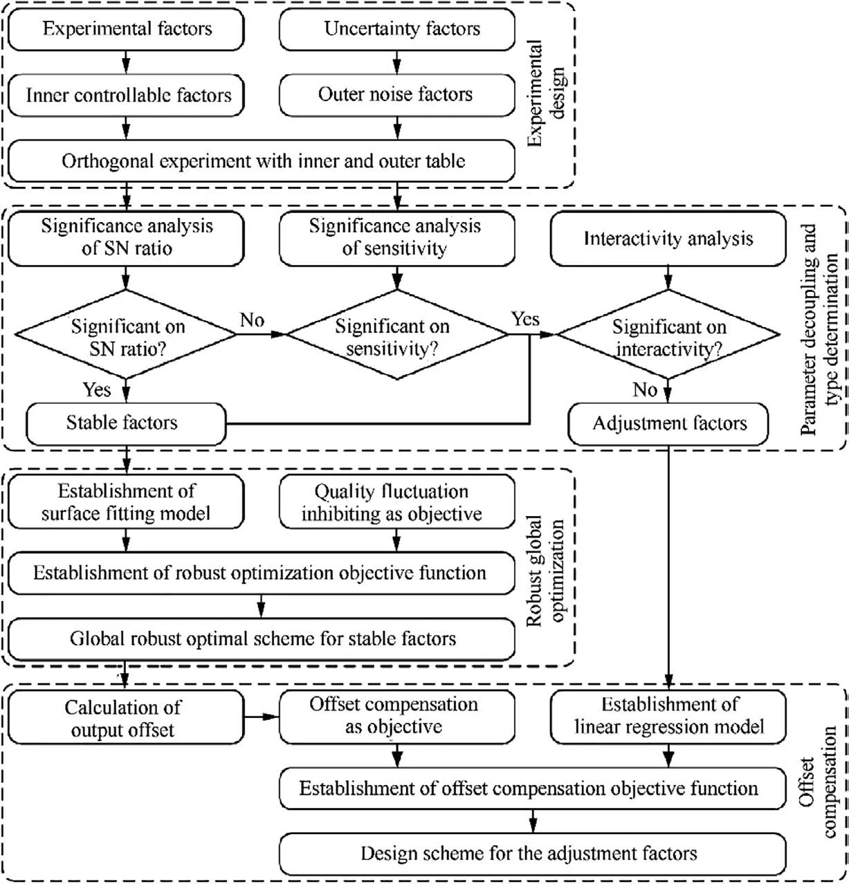
Fig. 1 Procedure of RPD proposed in the paper.

Thirdly, the nonlinear functions between the stable factors and output characteristics are established based on the polynomial fitting. With the purpose of reducing the quality fluctuation,the robust optimization objective is established,and then the scheme of stable factors can be obtained by the global optimization to minimize the change rate of output (i.e. the standard deviation).

Lastly,the offset of output is calculated after the stable factors have been designed. Then the offset compensation objective is established by using the polynomial functions of adjustment factors. Thus, the design of adjustment factors can move the output (i.e. the mean) back to the target value.

3. Mathematical models for the proposed RPD method

3.1. Significance analysis

In Taguchi method,the impact of input parameters on the SN ratio and the sensitivity is calculated by the significance analysis. The SN ratio S is able to reflect the impeding ability of input parameters to output fluctuation when different values are selected, and its calculation formula is given in

is the average fluctuation of the output y.is the error variance,yjis the result of jth output value,y-is the average of output, m is the number of output.

The stable factors with strong nonlinear properties to the output are determined if they have significant impacts on the SN ratio. By moving their values into a nonlinear interval,the stable factors can improve the robustness of output effectively.

The sensitivity η is used for reflecting the influence of input parameters on output amplitude when different values are selected, and its calculation formula is expressed as

The adjustment factors with approximately linear properties to the output are determined if they have insignificant impacts on the SN ratio and simultaneously have significant effects on the sensitivity. When output characteristics deviate from the target value, the adjustment factors can easily compensate the offset.

The calculation processes of SN ratio and the sensitivity are achieved through the outer design of crossed-array orthogonal method, in which experimental factors are the uncertainties(i.e. the fluctuation ranges of input parameters). Then the calculation results are filled into the inner orthogonal table, in order to analyze the impact of input parameters on the SN ratio and the sensitivity by the ANOVA analysis.

3.2. Interactions analysis

For the purpose of global optimization when factors vary continuously in the interval of the solution,it is necessary to accurately establish a relationship between input parameters and output characteristics in the form of a function.Due to a large number of input parameters and the nonlinear effect between inputs and outputs,it is complex and difficult to directly establish a mathematical model with high precision. On the other hand, there are correlative and interactive influences generally existing among the input parameters. In order to avoid the determined optimal solution of stable factors to be affected during the process of output compensation,the independences should exist between the selected adjustment factors and stable factors. Therefore, in this paper, the experimental factors are separated by means of the interactions analysis method to allow the determined adjustment factors to be mutually independent of the stable factors,and thus to establish the polynomial function models respectively.

Any two factors (X, Y) that are not duplicated are randomly selected from the experimental factors. First of all, the variations of the output characteristics Δx and Δy corresponding to the change of factor X and factor Y are calculated respectively.Then the variation of the output Δxy is computed when the factors of the combination (X, Y) are changed synchronously. In case factors X and Y are entirely independent,mathematical relation Δxy=Δx+Δy is satisfied. Otherwise,the two factors are considered to be interactive.

In addition, the factor γ is introduced to reflect the degree of interaction,and Eq.(3)is utilized to measure the interaction effect among the factors.

3.3. Establishment of RPD objective functions

The curvilinear polynomial function of single independent stable factor can be established by using the least square method, Lagrange polynomial method, Newton iteration method, Jacobi iterative method, etc. However, for the stable factors with interaction, a surface interpolation or fitting method is required to establish the polynomial function model,such as Response Surface Method(RSM),Radial Basis Function (RBF), Kriging and other traditional modeling methods.Then the accuracy of the function models needs to be tested.For example, in the goodness-of-fit test, the determination coefficient and regression standard deviation are applied in order to verify the fitting degree of the model to sample observations.

With the purpose of impeding quality fluctuations during the process of robustness optimization, the polynomial functions of stable factors are utilized for the determination of optimal values in the solution region, in order to minimize the change rate of the output characteristics. The partial derivative of the stable polynomial function Fswith respect to each factor Xsis taken, in order to obtain the slope of the function in the direction of each factor. The closer the slope is to zero,the higher the stability of the function is.Therefore,the sum of squares of the slopes is calculated to establish the objective function Fsta.Consequently,the robustness optimization problem H1is transformed into the evaluation of the minimum value of the objective function Fsta, which may be written as

The linear regression method is adopted to establish the polynomial function between the adjustment factors Xaand output characteristics. Firstly, the offset ΔFsof the output is calculated after the values of stable factors are changed. Then the adjustment polynomial function Fais combined with the offset ΔFsto establish the offset compensation target H2,which may be expressed as

Because H2has multiple optimal solutions in theory, additional conditions can be added according to the practical problem, in order to determine the design scheme for the adjustment factors.

4. Case study

The balanced force electromagnetic relay is a typical and widely used electrical apparatus applied to aeronautical condition. The holding force of electromagnetic system in the relay is used as the objective function of robust optimization design,in order to verify the validity and correctness of the improved RPD method proposed in this paper.

The structure of electromagnetic system is depicted in Fig. 2, consisting of the iron core, coil, armatures, yokes, permanent magnet and shaft. When the coil is not energized, the magnetic flux provided by permanent magnet creates holding force between releasing armature and releasing yoke, in order to guarantee the vibration resistance of the armature under the release conditions.When the coil is carrying the rated current,a magnetic flux opposite to the direction of the permanent magnet will be generated in the magnetic circuit, in order to counteract the holding force between releasing armature and releasing yoke, and then drive the armature group to rotate around the shaft until the pickup armature and pickup yoke are fitting closely together. At this moment, the holding force between pickup armature and pickup yoke determines the vibration resistance of the armature under the pickup conditions.

In this paper, the release holding force of the electromagnetic system is selected as the objective for the RPD. In order to accurately obtain the relationship between design parameters and release holding force, the simulation modeling is adopted for the calculation.

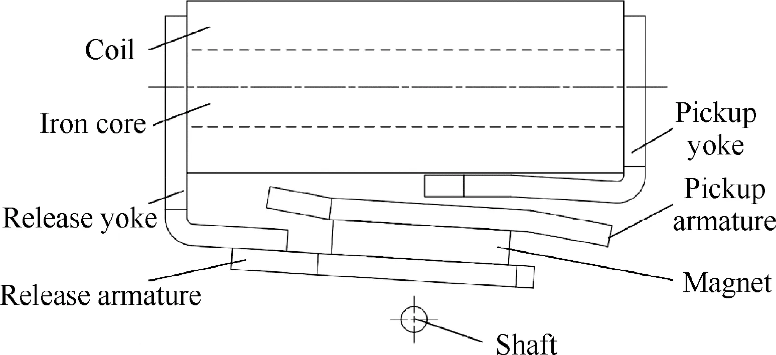
Fig. 2 Structure of an electromagnetic system.

4.1. Orthogonal experimental design

After the preliminary theoretical analysis, six design parameters in the electromagnetic system are chosen as the experimental factors of the RPD. The central values and tolerances of experimental factors are displayed in Table 1.

4.1.1. Inner design

Three level values are chosen respectively for each controllable factor,in order to conduct the inner orthogonal design.As stated above, the purpose of orthogonal experiment in the improved RPD is only to confirm the type of factors. Therefore, two levels can be selected for each factor. However, in order to compare the optimization effect of the traditional and the improved method, three levels are chosen for the traditional methods to achieve the desired effect.The level values of the controllable factors are shown in Table 2.

The inner orthogonal table is chosen as L18(37). The number 3 denotes that each factor in the orthogonal table can take three level values. The number 7 denotes that this orthogonal table can accept up to seven experimental factors.The number of controllable factors in this paper is six, thus one factor can be left as an error term in the orthogonal table.The number 18 denotes that this orthogonal table consists of eighteen test schemes. The test scheme and results are shown in Table 3.

4.1.2. Outer design

To describe the impact of parameter fluctuations on the output characteristics, a set of outer orthogonal experiments corresponding to each scheme in the inner orthogonal table is designed respectively. Three level values are taken for each noise factor, namely the central value, the upper limit value and the lower limit value,as factor fluctuations in the tolerance range, as shown in Table 4.

The orthogonal table L18(37)is selected in the outer design.Therefore, the total number of planned tests within the inner and outer design is 18×18. After computing the output of each experimental scheme via the simulation method, both the SN ratio and the sensitivity for each outer orthogonalscheme are calculated individually by using Eqs. (1) and (2)before being filled into the inner array, i.e. Table 3.

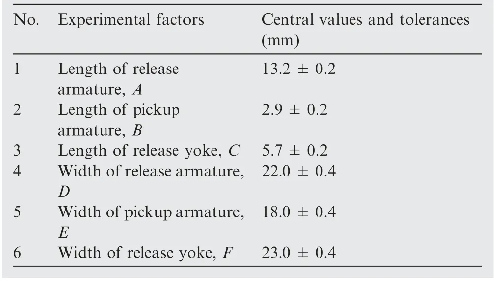
Table 1 Central values and tolerances of experimental factors.

4.2. Significance analysis

The significance analysis for the SN ratio and the sensitivity in Table 3 are conducted by using the ANOVA method. Subsequently, the controllable factors can be confirmed according to the analysis results, which are presented in Tables 5 and 6, where e is experimental error, T is total of results, STis sum of squares of fluctuations, dfis degree of freedom, MS is mean square, F value is the ratio of factor’s MS to error’s MS, P is the result of P-tests according to F value.

In accordance with the significance analysis results in Table 5, factors D and F are determined to have nonlinear properties,and are referred to as stable factors.After combining this with the analysis results from Table 6,it can be verified that the factors A,C and E have approximately linear properties and great impacts on output.

For the sake of comparing the optimization accuracy of the traditional and the improved method,the traditional method is utilized first to obtain the optimal solution(as shown in Table 7 and marked with‘‘△”in Fig.3,where‘‘°”represents the result of the Original scheme).Regarding the stable factors D and F,the optimal values are determined as the level value, whose partial sum(the average value of the SN ratio results in Table 3 corresponding to the equal level value) is the maximum value in all three levels. The calculated partial sum and the optimal values of stable factors are displayed in Table 7.

4.3. Interactions analysis

In order to identify the adjustment factors among the factors A, C and E, which are independent of the stable factors D and F, the interactions among experimental factors are analyzed. The scheme of factor changes is shown in Table 8.

Firstly, the output of release holding force is calculated when each factor takes the central value. Next, two arbitrary factors are combined to calculate the output in cases when factors are varying separately and simultaneously.The results are shown in Table 9.

Finally, the interactions analysis results are calculated by using the Eq. (3). After setting the interaction factor γ to 10%, the obtained analysis results are stated in Table 10.

From the analysis results,it can be seen that there is a very strong interaction between stable factors D and F.Thus,if the robust optimal solutions for factor D and F are determined separately, the interaction between factors will definitely carry a huge impact on the accuracy of the optimization.Therefore,a polynomial function must be established for these two factors, and their optimal solutions should be synchronously determined.

In addition, there is a strong interaction between factor D and E, which means the compensation of output using factor E can have an influence on the robust optimization results.The factors A and C are mutually independent of factors D and F, and thus can be used as the adjustment factors. Meanwhile,there is a mutual independence between factors A and C.Consequently, polynomial models for A and C can be established separately.

Table 2 Levels of controllable factors.

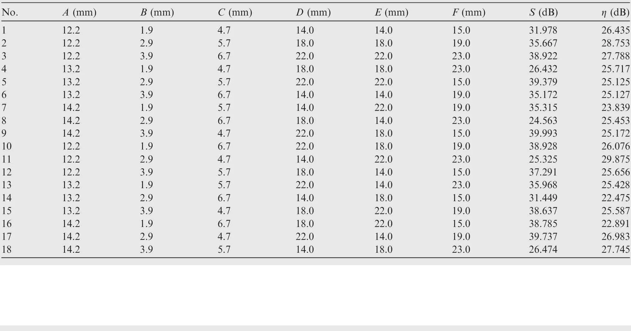
Table 3 Inner orthogonal test scheme and the results.

Table 4 Levels of noise factors.

Table 5 Variance analysis results of SN ratio.

Table 6 Variance analysis results of sensitivity.

Table 7 Calculation results of SN ratio and optimal level of stable factors.

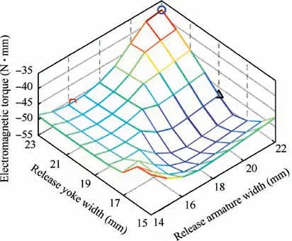
Fig. 3 Sampling points and computational results of stable factors.

Table 8 Scheme of factor changes.

4.4. Establishment of polynomial functions

4.4.1. Polynomial function of stable factors

First of all, equidistant sampling within the solution range is adopted to intuitively determine the stability region of stable factors D and F on the output characteristics. Secondly, sampling points are selected in the stability region to model the polynomial function for stable factors. Aiming to obtain the solution in the region of factor D [14,22] and in the region of factor F [15,23], nine uniformly spaced values are selected as samples. Thus, the total amount of sampling points is 81.The computational results are presented in Fig. 3.

According to the varying behavior of the curved surface in Fig.3,the stability region with strong inhibiting ability on factor fluctuations is obtained, where more details can be seen in Fig. 4. Then, the sampling points are selected to establish a polynomial function indicating the impact of stable factors D and F on the output characteristic T, by means of RSM method. The function model is given in Eq. (6).

Fig. 5 shows the comparative analysis of the polynomial function with the data of sampling points. Besides, the goodness-of-fit method is applied to evaluate the fitting degree of the polynomial model to sampling points. Thereat, the determination coefficient R2refers to the proportion of Sum of Squared Residuals (SSR) in the Sum of Squares for Total(SST), whose value range is [0, 1]. The closer the value is to 1, the higher the fitting precision of the polynomial function is. The calculation result of R2for Eq. (6) is 0.997, which is acceptable. Therefore, the polynomial function can be applied to the robust parameter optimization.

4.4.2. Polynomial functions of adjustment factors

As shown in Figs. 6(a) and (b), 5 uniformly spaced values within the variable range are selected respectively for the adjustment factors A and C, in order to establish the polynomial functions of adjustment factors to the output characteristic T, by means of least-square curve fitting method.

The variable range of the factor A is [12.2, 14.2], and the variable range of factor C is [4.7, 6.7]. The polynomial functions are shown in Eqs. (7) and (8).

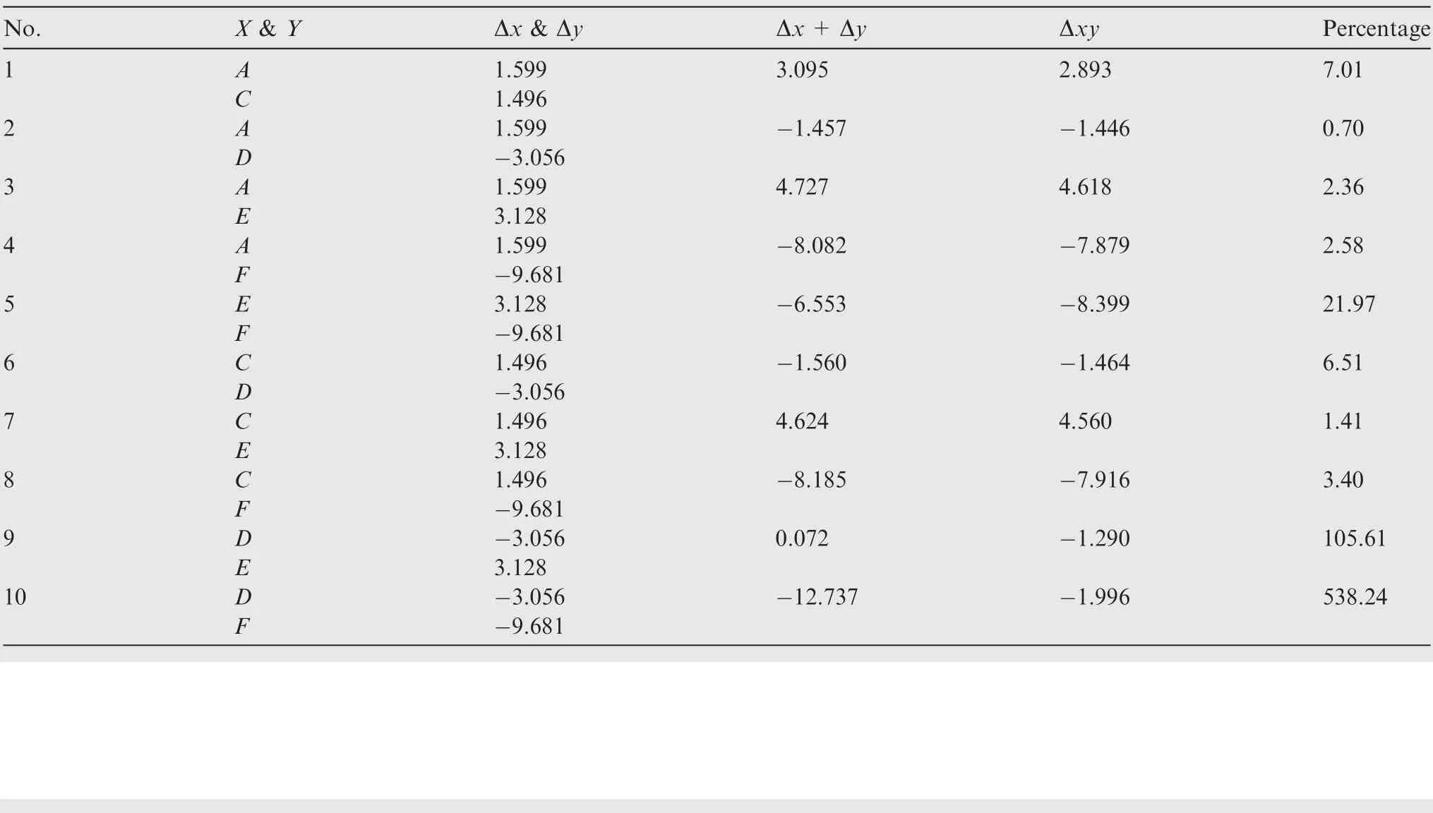
Table 9 Calculation results of factors varying.

Table 10 Interactions analysis results.

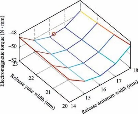
Fig. 4 Stability region of stable factors.

It can be proved that the determination coefficients R2of adjustment polynomial functions are 0.985 and 0.997 respectively, which satisfies the precision requirements.

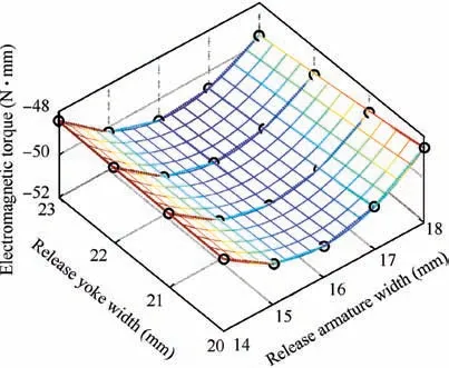
Fig. 5 Comparison of stable polynomial function with data of sampling points.

4.5. Establishment of objective functions

For the purpose of determining the optimal solution for the polynomial function of stable factors D and F in the solution domain,the objective H1for the RPD is established according to the Eq. (4) and expressed as

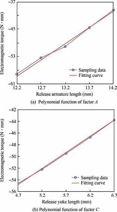
Fig. 6 Comparison of adjustment polynomial functions with data of sampling points.

Using the Sequential Quadratic Programming (SQP) algorithm, the optimal scheme for stable factors is obtained, leading to the minimum value of the objective function Y, as shown in Eq. (10). The obtained result is marked with ‘‘□”in Fig. 3.

The release holding force of the electromagnetic system under the original scheme is -37.808 N·mm, and the output after the optimazation of stable factors is calculated to be-50.906 N·mm. Therefore, the offset of the output is gained to be ΔT=13.098 N·mm.

Combining the polynomial Eqs.(7)and(8),the offset compensation objective H2is established according to the Eq. (5).The target H2is expressed as

As mentioned above, the objective H2theoretically has multiple sets of solutions. Therefore, additional conditions need to be added according to the practical problem. In this case, as the length of armature varies, the rotational inertia of movable parts changes proportionally, which can affect the operation of relay. Therefore, the minimum change of armature length min{ΔA} is defined as the additional condition and added to Eq. (11). Then the optimization scheme for adjustment factors is calculated as

4.6. Verification

Using Monte Carlo stochastic simulation method, the quality distribution characteristics before and after the RPD is performed, are analyzed and compared. Then, the mean value and the standard deviation are calculated by using statistical methods, in order to accurately evaluate the quality consistency of the design schemes, and also to quantitatively compare the improvement with the traditional RPD method and the improved RPD method.

Firstly, on the basis of tolerance range of each design parameter in the electromagnetic system, 50 values possessing normal distribution are randomly generated using the independent identically distributed central-limit property. Next, the values of 6 design parameters are randomly combined to generate 50 sets of virtual samples. Then the assembly dimension chain is applied to verify the validity of samples.In the end,the release holding force for each effective virtual sample is calculated via simulation,and thereat to obtain the quality distribution characteristics of the design schemes. As a result, the quality distributions respectively corresponding to the Original scheme,the Modified scheme with the improved RPD method,and the Traditional scheme with the traditional RPD method are displayed in Fig. 7.

In order to compare the quality fluctuations of the above three schemes more intuitively, the three distribution characteristics in Fig. 7 are respectively shifted to zero on the mean value, as shown in Fig. 8.

Under the condition of tolerances being constant,the traditional RPD method is capable of reducing the standard deviation of output characteristics from 0.714 to 0.530, with a decreased magnitude of 25.8%. It proves that the traditional method is practically able to enhance the quality consistency of products.

Using the improved RPD method proposed in this paper,the standard deviation is reduced to 0.194 before the offset compensation, with a decreased magnitude of 72.8%(increased by 47% compared to the traditional method). It demonstrates that the improved method can better exploit the nonlinear effect between design parameters and output characteristics, in order to effectively increase the robustness and consistency of products.

After changing the values of stable factors,the central value of output characteristic deviates accordingly. Using the previously determined adjustment factors to compensate the offset,the central value of output changes to-38.35,with an error of 1.43% to the target value -37.81. The quality distributions respectively corresponding to the Original scheme, the Modified scheme before output compensating and the Adjusted scheme after output compensating are displayed in Fig. 9.

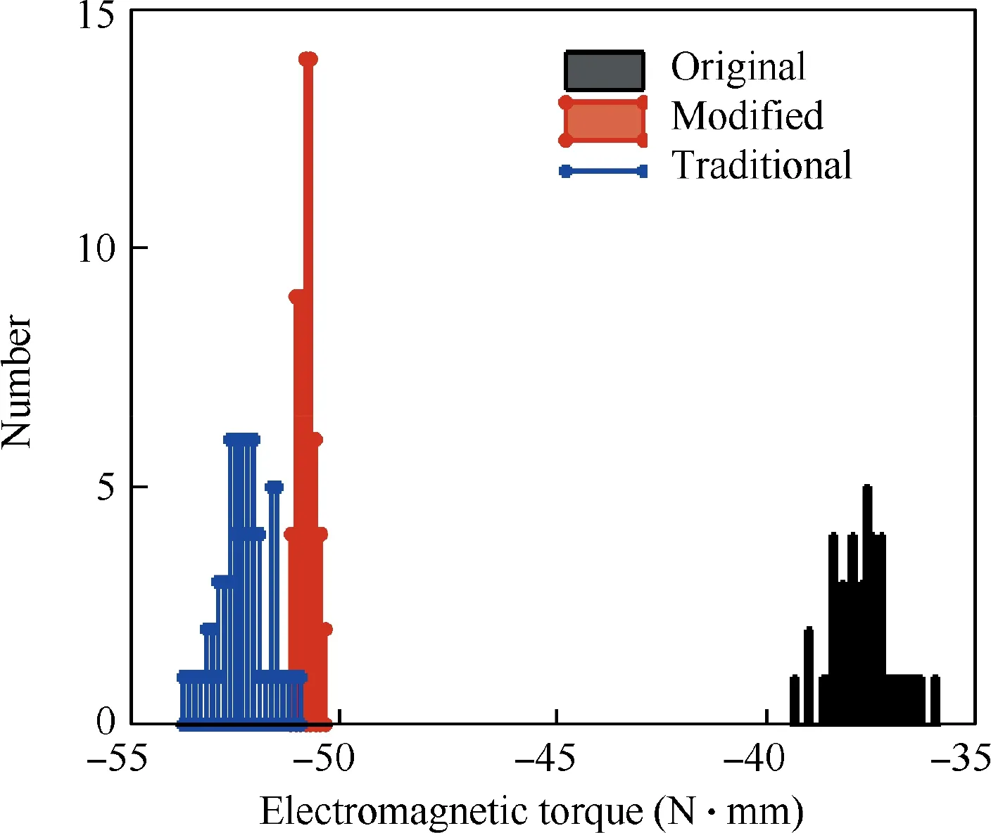
Fig. 7 Comparison of quality distributions with Original,Modified RPD and Traditional RPD schemes.

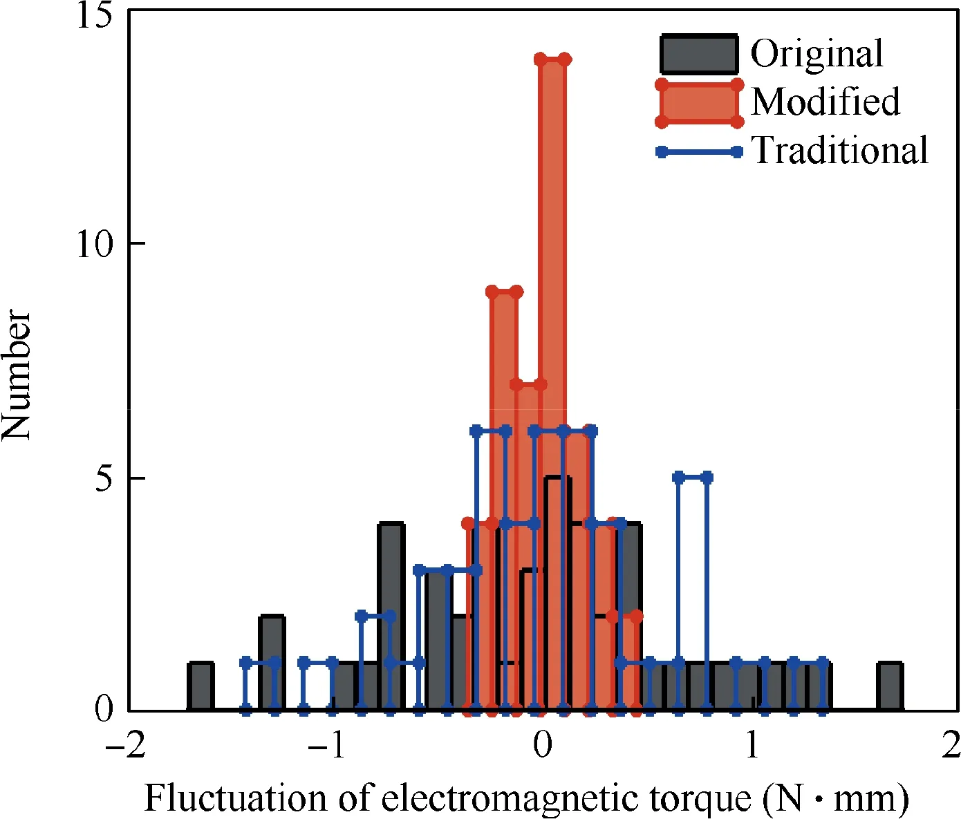
Fig. 8 Comparison of quality fluctuations with Original, Modified RPD and Traditional RPD schemes.

By shifting the distribution characteristics in Fig. 9 respectively to the zero on the mean value, the quality fluctuations before and after the compensation are shown in Fig. 10.

The standard deviation of the output after the compensation is increased from 0.194 to 0.201, with a variation of 3.61%. The results show that the adjustment factors possess great linear properties and are independent to stable factors,being able to compensate for the output offset without impacting the robustness of schemes.

In addition, thirty actual products are selected from batch products separately before and after the RPD is performed,in order to confirm that the obtained results of design parameters from the proposed scheme are actually effective when being used in the manufacturing process. The mean value and the standard deviation of the quality distribution characteristics before and after the RPD are statistically calculated and compared, which are shown in Fig. 11 and Table 11.

Firstly, it can be seen from the results in Table 11 that the actual standard deviation of quality distributions before and after the RPD optimization are both larger than the theoretical results shown in Table 12.In theoretical analysis and optimization, only six main influencing parameters are selected. But in the actual manufacturing process,the fluctuation of all parameters including many uncontrollable noise factors, whether major or not, will affect the consistency of output. Therefore,it is reasonable that the actual standard deviation is larger than the theoretical one.

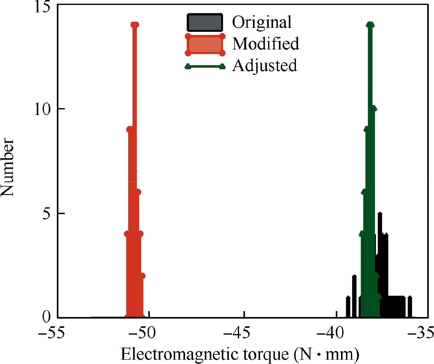
Fig. 9 Comparison of quality distributions before and after compensation for output offset.

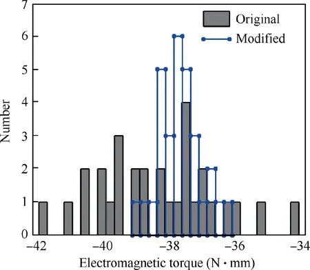
Fig. 11 Quality consistency of actual products before and after RPD is performed.

Table 12 Statistical results of quality distribution characteristics before and after the RPD is performed.

Secondly,the standard deviation of actual quality distribution is significantly reduced by 62.9% after the RPD is performed, which means the expected satisfactory performances can be actually realized by the proposed RPD method.

5. Conclusions

It is hard for the traditional RPD method to obtain the globally optimal solution,which significantly reduces the optimization effect of robustness and consistency. This paper puts forward an improved RPD method based on interactions analysis and polynomial fitting.

(1) Through the interactions analysis,it enables the selected stable factors and adjustment factors to be mutually independent, and consequently to establish the polynomial functions between factors and output characteristics respectively. By this means, it reduces the number of input parameters during the functions establishing process, thereat evidently lowering the modeling difficulty, decreasing the number of sampling points and improving the modeling precision.

(2) By using the polynomial function of stable factors, the proposed method can take full advantage of the nonlinear relationship between design parameters and output characteristics, in order to obtain the global optimal solution of RPD. Demonstrated by the example given in this paper,the improvement of robustness and consistency with the improved method is 46% more than the one with the traditional method.

(3) By using the polynomial functions of adjustment factors, it is able to adjust the offset of output characteristics without affecting the robustness of the optimization schemes. In the presented example, the error of the offset compensation is 1.43%, and the amplitude of influence of the offset compensation process on the consistency of the design scheme is only 3.61%.

(4) The RPD method proposed in this paper focuses on the improvement of the design process. Therein, the approaches adopted in each stage of the optimization process are not limited to the methods used in this paper, but can be adjusted and replaced according to the practical applications. Therefore, this method has a good applicability.

Acknowledgements

This study was co-support ed by the National Natural Science Foundation of China (Nos. 51707044 and 61671172) and the China Postdoctoral Science Foundation (No. 2018M632377).