The Modified Local Crank-Nicolson Schemes for Rosenau-Burgers Equation

Muyassar Ahmat, Abdurishit Abduwali, Abdugeni Abduxkur

(1- College of Mathematics and System Science, Xinjiang University, Urumqi 830046;2- College of Mathematics and Statistics, Yili Normal University, Yining 835000)

Abstract: Two class of modified local Crank-Nicolson schemes for Rosenau-Burgers equation are proposed.Firstly, we obtain the exact solution of the ODE which reached from the original PDE by using central finite difference discretization in space direction.Next, the exponential coefficient matrix of this equation is approximated by using matrix splitting technique by line and element.Finally, two types of methods are achieved by using modified local Crank-Nicolson scheme.The stability,convergence and priori error estimation of two schemes are discussed.The accuracy of theoretical proof and efficiency of both schemes are demonstrated by numerical results.The proposed methods possess the advantages of simple structure and high accuracy.

Keywords: Rosenau-Burgers equation;Crank-Nicolson method;modified local Crank-Nicolson scheme

1 Introduction

In the study of discrete dynamics system, the physical interaction of wave-wave or wave-wall collision can not well described by well-known KdV equation which was presented by Korteweg and de Vries[1].To solve this problem, Rosenau proposed Rosenau equation[2].

However, Rosenau-Burgers equation was presented by adding-uxxin order to further consider the loss of power system in space[3].

The existence and uniqueness of the solution for (2) was proved by [4].Since then, much work has been done on the numerical method for (2) with the boundary conditions

and the initial condition

Many effective finite difference methods[5-12]have been used to approximate the exact solution.Huet al[5]proposed a nonlinear Crank-Nicolson difference scheme for the Rosenau-Burgers equation which have to be solved with Newton iterative algorithm.Liet al[6]came up with a linear three-level finite difference scheme with the advantage of its convenience to solve the problem without iteration.A second-order accurate linearized difference scheme was applied by [7].A linear three-level average implicit finite difference scheme is introduced by [8].

Researchers also work on the generalized Rosenau-Burgers equation.Zheng and Hu[9]presented nonlinear two-level Crank-Nicolson difference scheme for the Generalized Rosenau-Burgers equation.An average implicit linear difference scheme is used for this equation by [10], Xue and Zhang[11]proposed a two-level linear implicit finite difference scheme, which can reduce the computational work and be easily implemented.Zhou and Zheng[12]also contributed to the study of generalized Rosenau-Burgers equation.

In this paper, two types of modified local Crank-Nicolson methods which has been designed by Abduwali in order to solve the two-dimensional heat transfer equation in[13]Burgers equations in 1D and 2D by [14]are achieved to solve Rosenau-Burgers equation.

2 The modified local Crank-Nicolson schemes for Rosenau-Burgers equation

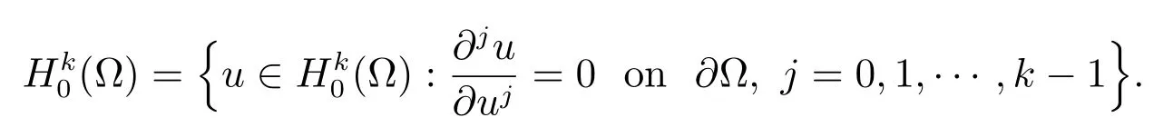
We define the solution domain to beQ={(x,t)|0≤x ≤L, 0≤t ≤T}, which is covered by a uniform gridQh={(xi,tn)|xi=(i-1)h,tn=nτ,i=1,2,···,M,n=0,1,···,N}.HereDenote{u=(ui)|u1=uM= 0,i= 1,2,···,M} andHk(Ω) denote the usual sobolev space of real-valued function defined on Ω by nonnegative integerk, define

It can be easily obtained by semi-discretion for (1) at (xi,t), we have

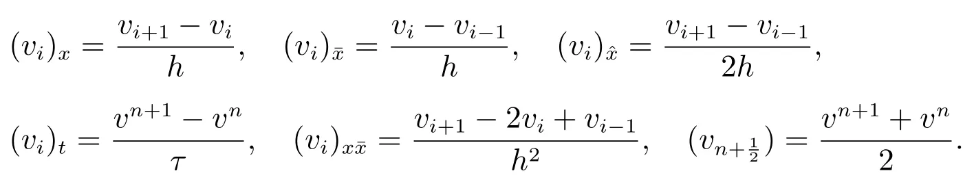
Next we define these following difference operators

We have

Its explicit expression is

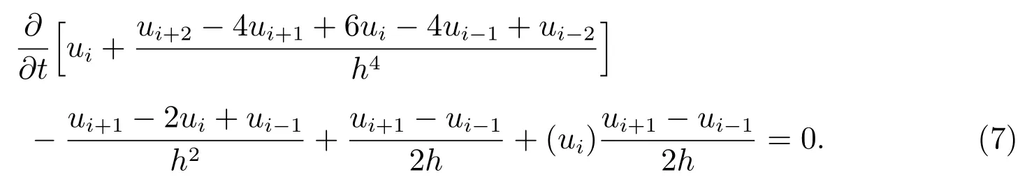
(7) also can be written into ordinary differential equation

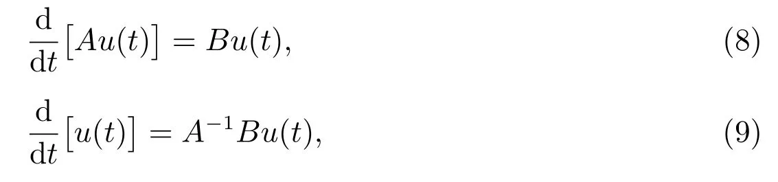
where

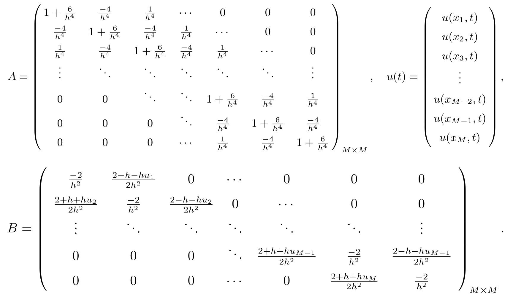
The exact solution of this ordinary differential equation (9) for initial conditionu(t0)=[u0(x1),u0(x2),···,u0(xM)]can be indicated as

Discrete the equation (1) at the point (xi,tn) based on former difference operators, we obtain

It can be reorganized as

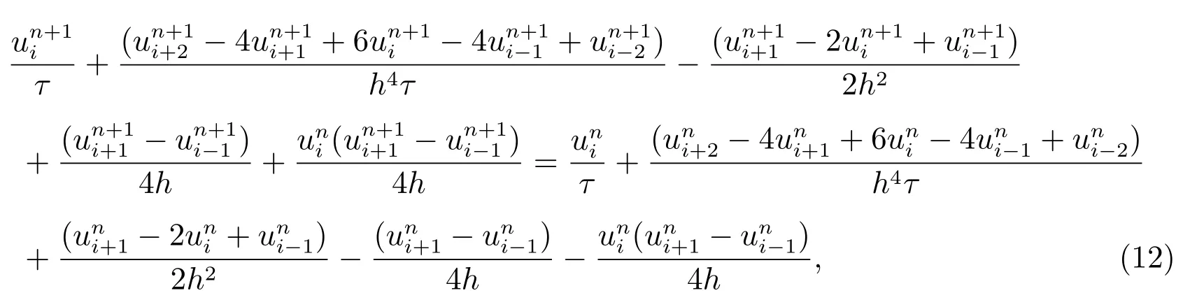
(12) also can be written as

We obtain following approximation from (10) and (12)

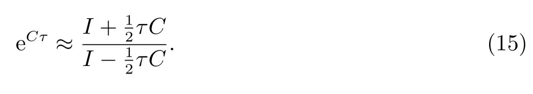
LetC=A-1B, then (14) can be rewritten as

Lemma 1(Abdirishit)[13]Express the matrixDin the form ofK ∈N+, we have

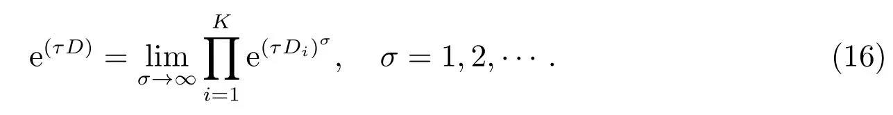
According to Lemma 1, we have

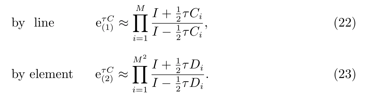
According to (17), we can split the matrixCby matrix line and matrix element,respectively.The first type of matrix split by line is given as follows

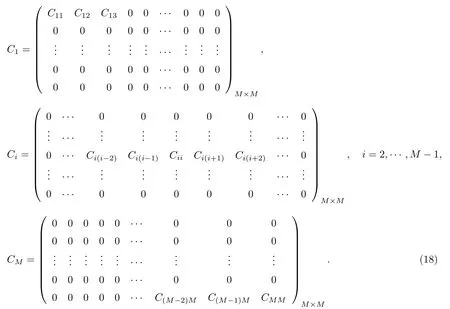
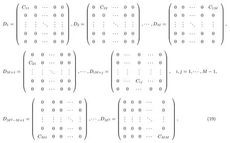
The second type of matrix split by element is given as follows

we obtain

It can be deduced from (17),(20) and (21)

We obtain two different kind of new difference schemes from (13) and (22),(23).

In order to improve the accuracy of (24) and (25), we defineEi=CM-i+1,Fj=DM-j+1,i=1,2,···,M,j=1,2,···,M2, and substitute in (24),(25)

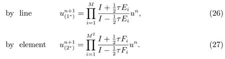
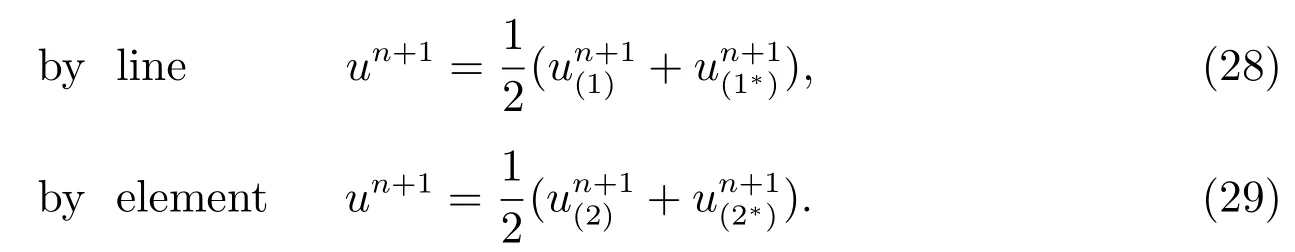
Finally, we obtain two different modified local Crank-Nicolson schemes based on line and element respectively by averaging (24),(26) and (25),(27).

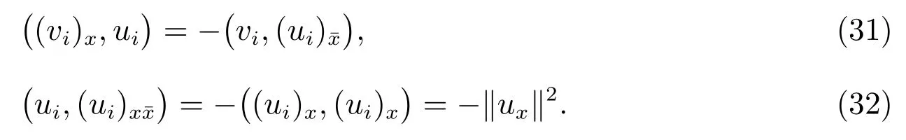
Lemma 2[5]For any two mesh functionsu,v ∈we have

Therefore,

Lemma 3(Discrete Sobolev’s inequality)[15]There exist constants such ask1,k2,such that

Theorem 1Supposethen there is an estimation forunsatisfies

which yield

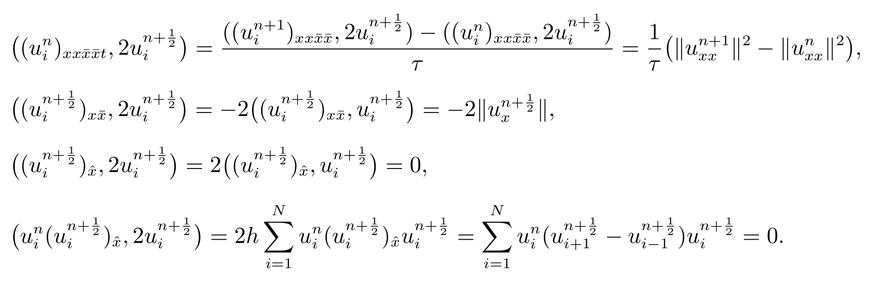
ProofConsider inner product withfor (11), we obtain

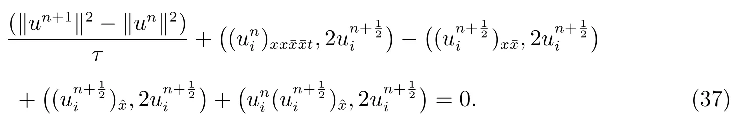
Considering the boundary condition (4) and Lemma 2, we have

Therefore, (37) can be rewritten as

then

Finally

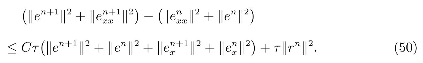
By using Lemma 2 and the Cauchy-Schwarz inequality, we derive

3 Solvability

It is necessary to apply Brouwer fixed point theorem for proof the solvability of(2)-(4).

Lemma 4(Brouwer fixed point theorem)[15]LetHbe a finite dimensional inner product space, suppose thatg:H →His continuous and there exists anα ＞0 such that (g(x),x)＞0 for allx ∈Hwith ‖x‖ =α.Then there existsx∗∈Hsuch thatg(x∗)=0 and ‖x‖∗≤α.

Theorem 2There existun ∈which satisfies (2)-(4).

ProofThe theorem is proved by mathematical induction,supposeu0,u1,···,un,n ≤N-1 satisfies (2)-(4).Next, we proofun+1also satisfies (2)-(4).Let

gis continuous,use the inner product for(11)withv,let=0,we have

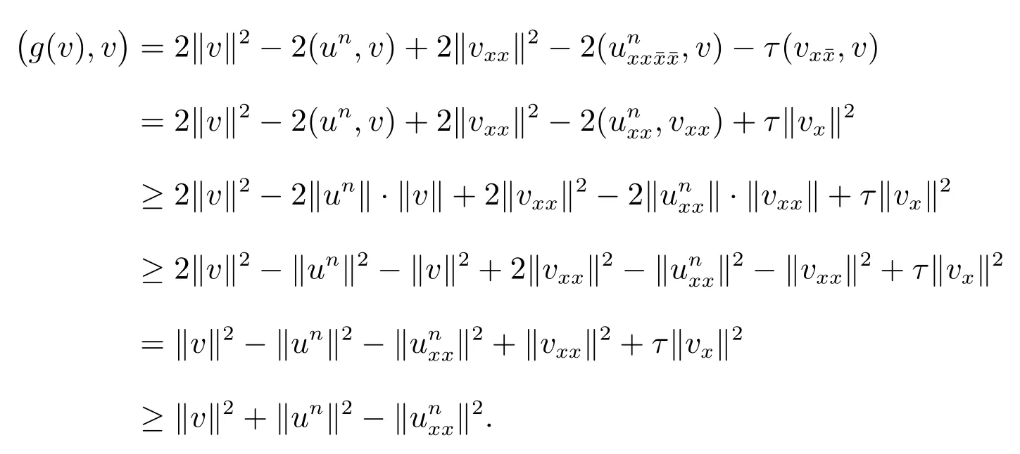
Therefore (g(v),v)＞0 for anyv ∈

According to Lemma 4, there existsv ∈such thatg(v∗) = 0.If we takeun+1=2vn-un, thenun+1satisfies (2)-(4).

4 Convergence and stability

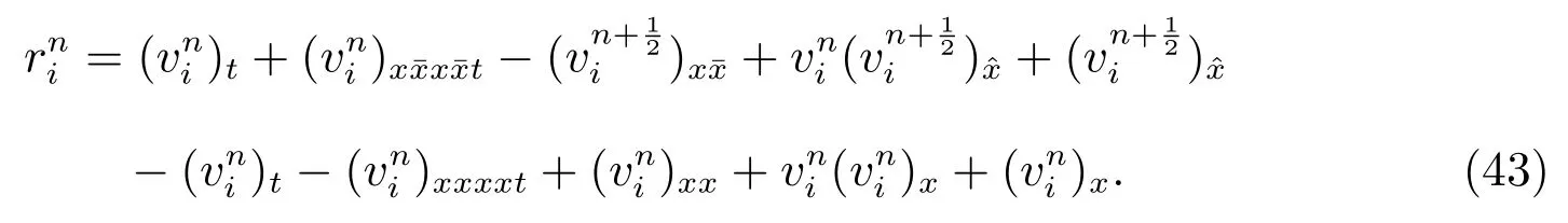
Letv(x,t) be the solution of problem (2)-(4),then the local truncation error of the difference scheme (11) is

According to Taylor expansion, we know thatholds ifh,τ →0.

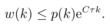
Lemma 5(Discrete Gronwall inequality)[15]Supposew(k),p(k) are nonnegative function andp(k) is nondecreasing.IfC ＞0, and

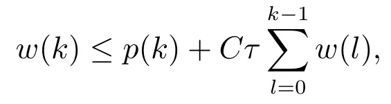
then

Theorem 3Supposeu0∈then the solutionunof the difference scheme(2)-(4) converges to the solutionv(x,t) of problem (2)-(4) in norm ‖·‖∞and the rate of convergence iso(h2+τ2).

ProofSubtracting (5) from (43) and lettingwe have

Let

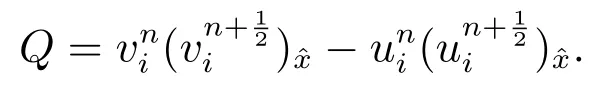
Computing the inner product of (44) withand usingwe obtain

That is

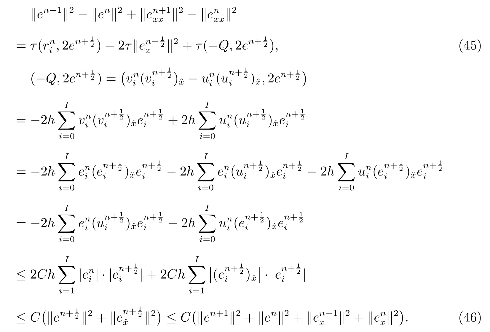
Noting that

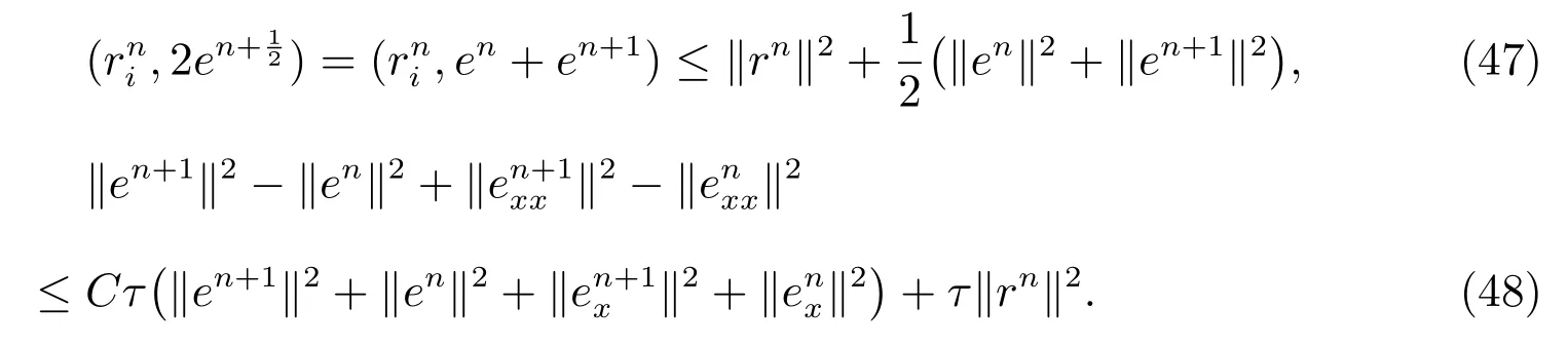
Similar to (41), we can prove

(48) can be changed into

Summing up (51) from 0 ton-1, we have

Noticing

We getB0=o(τ2+h2)2.Hence we obtain

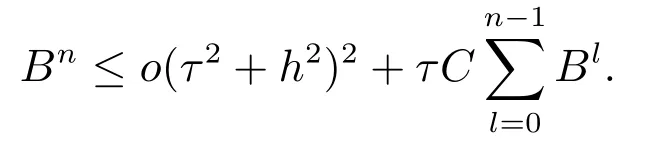
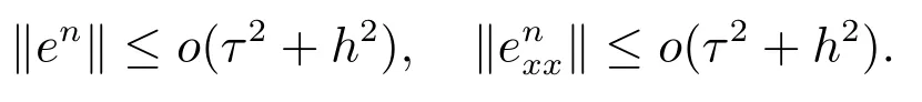
From Lemma 5, we getBn ≤o(τ2+h2)2.That is

Theorem 4Under the conditions of Theorem 3, the solution of (2)-(4) is stable for initial data in norm ‖·‖∞.

Theorem 5The solutionunof (2)-(4) is unique.

5 Numerical tests

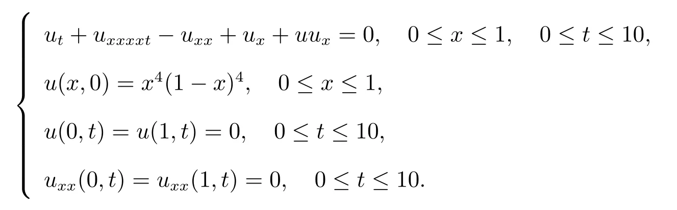
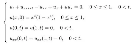
Example 1Consider the initial boundary problem of Rosenau-Burgers equation

Since we don’t know the exact solution of problem.In order to obtain the error estimation, we consider the solution on meshas the reference solution.The maximum errors from the two schemes in the article are presented in Table 1.

Table 1: The comparison of numerical results of (28) and (29) for Example 1 (h=τ =0.1, T =1)

Table 1: The comparison of numerical results of (28) and (29) for Example 1 (h=τ =0.1, T =1)

x (28)absolute error (29)absolute error exact solution 0.2 5.8509e-4 3.8317e-5 5.9195e-4 3.1456e-5 6.2341e-4 0.4 3.1731e-3 5.3479e-5 3.1874e-3 3.9254e-5 3.2266e-3 0.6 3.1733e-3 5.3377e-5 3.1874e-3 3.9281e-5 3.2266e-3 0.8 5.8513e-4 3.8283e-5 5.9195e-4 3.1458e-5 6.2341e-4 Max error 5.5534e-5 4.0067e-5

In Table 2,L2errors are given for (28),(29) in various time forwith fixedτ=0.05.

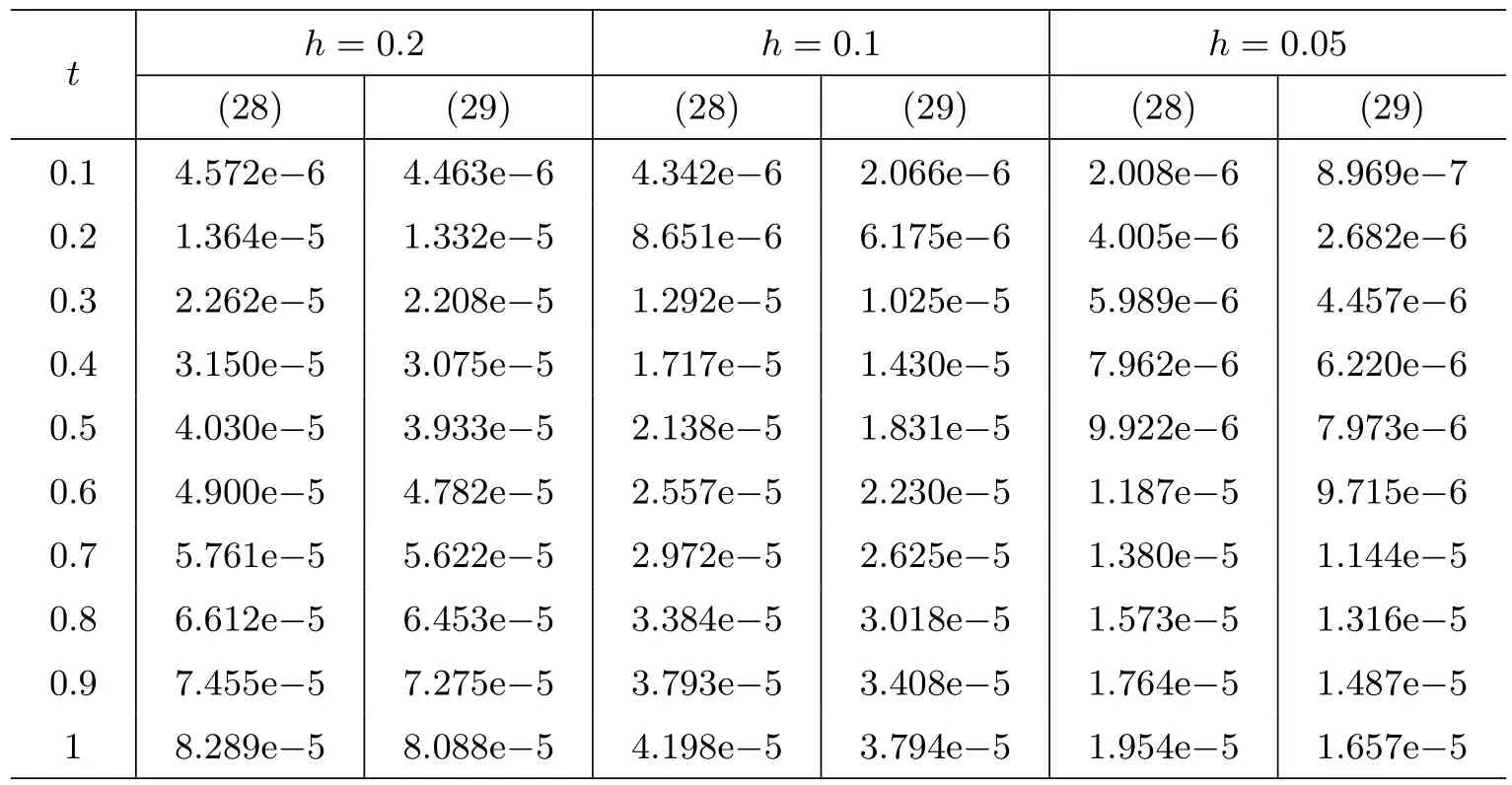
Table 2: The comparison of L2 error at various time step

The figure on the left of Figure 1 shows the numerical solutions of (28) and (29) ath=0.05,τ=0.05,T=1.It confirms that the approximated solutions are coinciding.The figure on the right of Figure 1 shows enlarged part in subsection in order to show the superiority of (29) more clearly.Figure 2 show the numerical comparison of (28)withτ= 0.1,h= 0.01 atT= 0,2,4,6,8 and 10, respectively.It is clear that the amplitude of the numerical solution decreases over time.

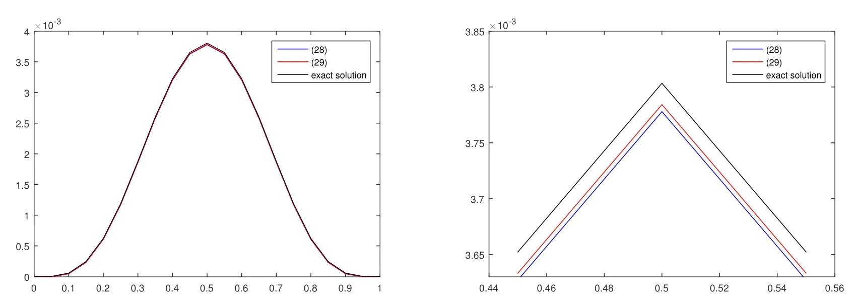
Figure 1: Numerical and exact solutions of (28),(29) in Example 1 at T =1 for h=0.05, τ =0.05

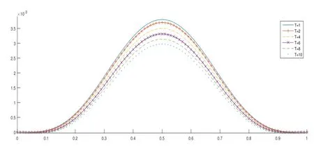
Figure 2: Numerical solutions of (28) in Example 1 at T =1,2,4,6,8,10 for h=0.01, τ =0.1

Example 2

In Table 3, the maximum errors of four schemes are presented, it is clear that our schemes give better approximation than other two schemes proposed in [5,7].The scheme splitting by element in this paper gives better results than the scheme splitting by line.It is also illuminated in Figure 3.

Table 3: The absolute max error comparison of four difference schemes at T =1

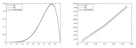
Figure 3: Numerical and exact solutions of (28), (29) in Example 2 at T =1 for h=0.05, τ =0.05

6 Conclusion

In this work, the studied equation is transformed into ordinary differential equation, then we use the Trotter product formula of exponential function to approximate the coefficient matrix, the five diagonal sparse matrix is summed of some simple matrices according to rows and elements.Finally two types of modified local Crank-Nicolson schemes for solving Rosenau-Burgers equations are presented by using the Crank-Nicolson method.In order to verify the effectiveness of the two numerical schemes,two numerical examples are given for numerical experiment.Numerical simulations show that these methods are efficient.