Convergence Properties of Local Defect Correction Algorithm for the Boundary Element Method

Godwin Kakuba,John M.Mango and Martijn J.H.Anthonissen

1 Makerere University,P.O.Box 7062,Kampala,Uganda.

2 Eindhoven University of Technology,P.O.Box 513,5600 MB Eindhoven,The Netherlands.

Abstract: Sometimes boundary value problems have isolated regions where the solution changes rapidly.Therefore,when solving numerically,one needs a fine grid to capture the high activity.The fine grid can be implemented as a composite coarse-fine grid or as a global fine grid.One cheaper way of obtaining the composite grid solution is the use of the local defect correction technique.The technique is an algorithm that combines a global coarse grid solution and a local fine grid solution in an iterative way to estimate the solution on the corresponding composite grid.The algorithm is relatively new and its convergence properties have not been studied for the boundary element method.In this paper the objective is to determine convergence properties of the algorithm for the boundary element method.First,we formulate the algorithm as a fixed point iterative scheme,which has also not been done before for the boundary element method,and then study the properties of the iteration matrix.Results show that we can always expect convergence.Therefore,the algorithm opens up a real alternative for application in the boundary element method for problems with localised regions of high activity.

Keywords: Local defect,defect correction,composite grids,integral equation methods,boundary elements.

1 Introduction

Often boundary value problems have small localised regions of high activity where the solution varies rapidly compared to the rest of the domain.This behaviour may be due to boundary conditions or due to an irregular boundary.One therefore has to use relatively fine meshes to capture the high activity.Since the activity is localised,one may also choose to solve on a uniform structured grid.The size of each grid is chosen in agreement with the activity of the solution in that part of the domain.The solution is thus approximated on a composite grid,which is the union of the various uniform local grids.One way of approximating this composite grid solution that is simple and less complex than directly solving on the composite grid is byLocal Defect Correction(LDC).This approach is well developed and extensively studied in methods like the finite difference methods(FDM)[Anthonissen,Bennett and Smooke(2005);Ferket and Reusken(1996);Hackbusch(1984)].In Kakuba et al.[Kakuba and Anthonissen (2014)],a local defect correction algorithm for the boundary element method(BEM)is presented.It was shown therein that the algorithm is cheaper than solving directly on the composite grid.The BEM,being a method with full matrices,would benefit much from such an algorithm when solving problems with localised regions of high activity that occur at the boundary.

The LDC technique employs a uniform global coarse grid that covers the whole boundary and then a uniform local fine grid in a small part of the boundary that contains the high activity.In Ferket et al.[Ferket and Reusken (1996);Hackbusch (1984)] LDC has been shown to be a useful way of approximating the composite grid solution in which a global coarse grid solution is improved by a local fine grid solution,through a process whereby the right hand side of the global coarse grid problem system of equations iscorrectedby thedefectof a local fine grid approximation.The properties for this method in FDM have been well studied,see for instance[Anthonissen(2001);Ferket and Reusken(1996);Hackbusch(1984);Minero,Anthonissen and Mattheij(2006)].Literature is still scanty on the LDC technique for BEM,but error studies,especially for direct multigrid applications,are increasing [Qu and Cui (2014)].A good overview is also given in Feischl et al.[Feischl,Führer,Heuer et al.(2015)].The LDC technique will be particularly useful in applications for problems that exhibit multiscales in behaviour.An example is the modelling of impressed current cathodic protection systems where the potential problem is characterised by small regions of high activity,cathodes and anodes.

In this paper we study convergence properties of the LDC algorithm for BEM which,to the best of our knowledge,has not been done.In Kakuba et al.[Kakuba and Anthonissen(2014)],the algorithm is presented using integral formulations.In this paper we base on the integral formulation to derive the corresponding fixed point iterative scheme in matrix form.This formulation assumes the boundary and the discretisation are such that,on refinement,the nodes of the global grid in the refinement area also belong to the fine grid.For the sake of completeness,we first briefly outline the development of BEM in Section 2.To build the discussion for the convergence properties,the important steps of the LDC technique for BEM,as published in Kakuba et al.[Kakuba and Anthonissen(2014)]are presented in Section 3,with an example.In Section 4,the LDC algorithm is formulated as a fixed point iterative scheme on the basis of which convergence properties are tested using examples.We conclude the study with a summary of the findings,in Section 5.

2 The boundary element method

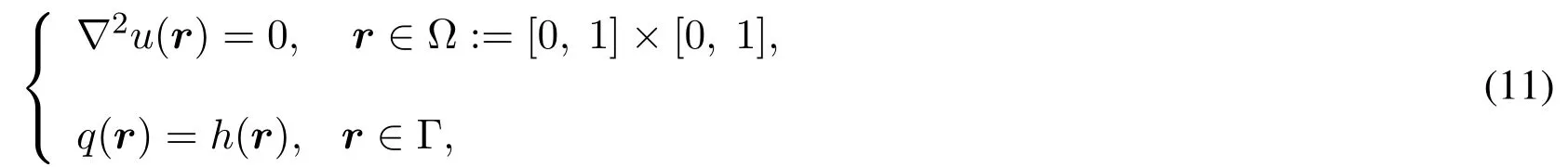
Consider a closed domain Ω⊂R2,with boundary Γ.Denote bynthe outward unit normal at Γ.We consider on Ω the two dimensional potential problem

for which Dirichlet,Neumann or mixed boundary conditions may be defined as illustrated in Fig.1.

Figure 1:Illustration of the domain Ω,with boundary Γ = Γ1 ∪ Γ2, Γ1 ∩ Γ2 = ∅,where on Γ1 we have Neumann boundary conditions,and on Γ2 we have Dirichlet conditions [Kakuba and Anthonissen (2014)]

If Γ1≡Γ,we have aNeumann problem,and if Γ2≡Γ,we have aDirichlet problemotherwise we have aMixed problem.In the solution of problem(1)using BEM,the problem is formulated as an integral equation

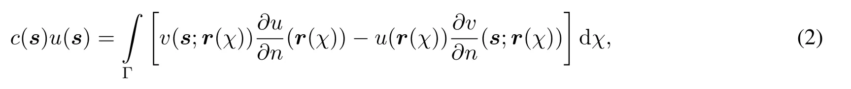
where the coefficientc(s)is given by,

whereris the variable field point,sis a fixed point,χa coordinate along the boundary,Ωcis the complement of Ω in R2andα(s) is the internal angle ats.The derivation of this boundary integral equation(BIE)is readily available [Katsikadelis(2002);Paris and Canas(1997);Pozrikidis(2002)].The functionvis the fundamental solution of the Laplace equation in R2given by:

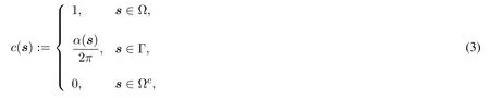
According to Eq.(2),the solutionucan be computed at any point in the domain if we knowuand its normal derivative everywhere at the boundary.The goal in BEM therefore is to look for the missing data at the boundary,which is the functionuat the Neumann boundary or the normal derivative∂u/∂nat the Dirichlet boundary.At the boundary,the discretised BIE leads to the linear system of equations

where

i,j=1,2,...,N,Γj,j=1,2,...,Nis a discretisation of Γ andNis the number of grid elements Γjused in the discretisation.We have also introduced the vectors

whereqis defined as

Using boundary conditions in Eq.(5)leads to the square system

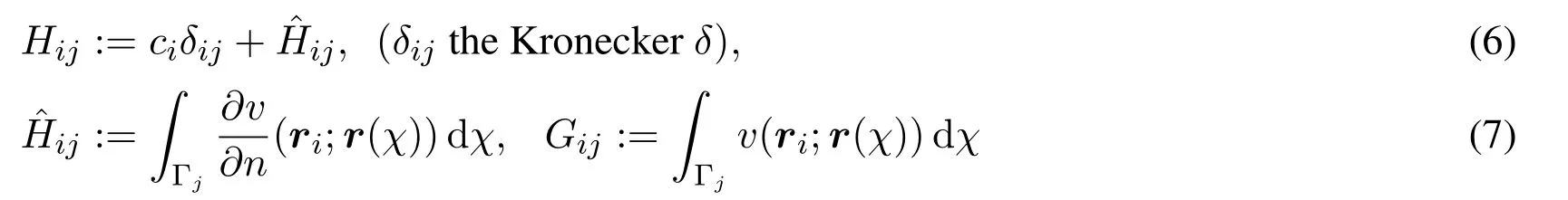
The vector x contains the unknown values of eitheruorqin the grid elements nodes at the boundary.The solution of the system(9)gives a BEM approximation of the unknowns in x in the grid nodes at the boundary.We denote by xLa BEM approximation on a grid of sizeL.Thus,uLj(orqLj)is a BEM approximation ofuj(orqj),using a grid of sizeL.Solving Eq.(9) gives the unknown boundary quantities ofuandq.Therefore,all the boundary quantities are available and the solutionuiat any pointri ∈Ω can then be computed using the identity

3 local defect correction

In this section we briefly present the local defect correction algorithm that was introduced in Kakuba et al.[Kakuba and Anthonissen (2014)].The presentation focusses on the important steps of the algorithm that are necessary in the development of the same,as a fixed point iterative scheme that is discussed in this paper.Consider the potential problem:

where

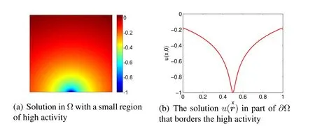
Figure 2:Solution in the domain,in 2(a),and solution at the boundary 0 ≤x ≤1,y =0,in 2(b),for problem(11)[Kakuba and Anthonissen(2014)]

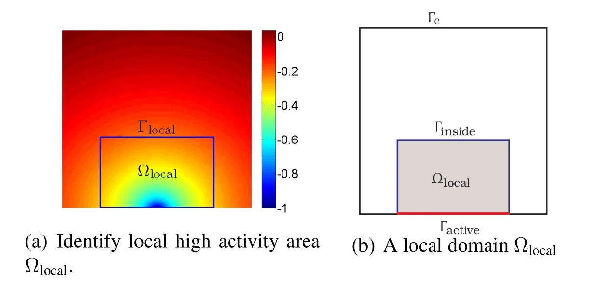
Figure 3:An example of a multiscaled solution with localised high activity,in 3(a) and,in 3(b),an illustration of a local problem domain.The boundary of Ωlocal is Γlocal :=Γactive ∪Γinside[Kakuba and Anthonissen(2014)]

The exact solution of this problem,shown in Fig.2,has a small area close to the boundary where it changes rapidly.As a result,the solutionu(r) at the boundary has a region of high activity in a small part of the boundary.The LDC algorithm distinguishes a small region of high activity in Ω and defines a local problem on it.We denote this region byΩlocal.Part of the boundary of Ωlocalintersects with the global boundary Γ,Fig.3.We call this intersecting part of the boundaries of Ω and Ωlocal,thelocal active boundary,Γactive,because it captures the high activity of the problem at the boundary.In the application of BEM to solve this Neumann problem,a Dirichlet condition is prescribed in one node,for uniqueness of results,which also enables us to compare the numerical results with the exact solution.In the LDC algorithm,alocal problemon Ωlocalis solved on a fine mesh whose size is chosen in agreement with the local activity.The solution on the local fine grid is combined with the solution on the global coarse grid,throughdefect correction,to obtain a composite grid solution on Γ.The global problem is solved on a uniformglobal coarse gridΓLofNelements each of sizeL,covering the whole of Γ,that is,

where|ΓLj|=Lfor allj= 1,2,...,N.The number of elements of the local problem is denotedNlocal,and the individual elements of the local grid are denoted Γllocal.Thus,the local problem is solved on Ωlocal,using a uniformlocal fine gridΓllocal,ofNlocalelements each of sizelcovering Γlocal.That is,

where|Γllocal,i|=lfor alli=1,2,...,Nlocal.This discretisation is illustrated in Fig.(4).In

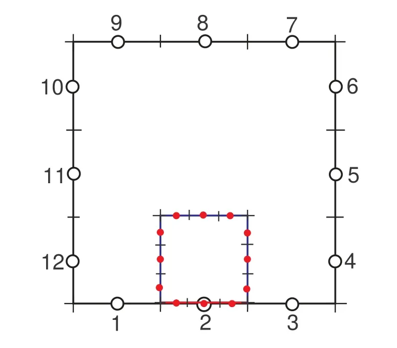
Figure 4:Global coarse and local fine grids.The dots are the nodes rllocal of the local fine grid Γllocal and the big open circles are the nodes rL of the global coarse grid ΓL.Node 2 belongs to rL ∩ rlactive [Kakuba and Anthonissen (2014)]

constant elements that we use here,the collocation nodes are the midpoints of the elements.Let

denote the set of coarse grid nodes.Let

be the set of the local fine grid nodes.Then we denote the nodes of the local problem that belong to the active part of the boundary asrlactive.We assume that all the grid nodes ofrL ∩rlactivebelong torlactive,Fig.4.The composite grid nodesrl,Lare the unionrL ∪rlactiveof the global coarse grid nodesrLand the active local fine grid nodesrlactive.First,we have the following discretised integral equation on ΓL

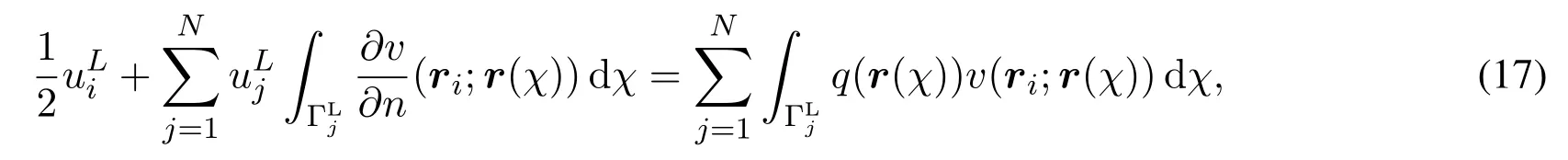
which leads to the initial global coarse grid system of equations

Note that on the right hand side of Eq.(17),the functionq(r) is given and,therefore,to make sure we are only measuring the errors due to the discretisation ofu,we minimise the interpolation error[Kita and Kamiya(2001)]by evaluating that integral without discretisingq,but by using an appropriate integration rule to evaluate that integral of the product ofqandv.Once Eq.(18)is solved,the solution is used to complete the formulation of the local problem by computinguon Γinsideto be used as the Dirichlet boundary condition.The local problem on Ωlocalsatisfies the same operator as in the global problem.Since Γactive⊂Γ,the boundary conditions on Γactiveare the same as those in the global problem.The local problem is solved on a finer grid and the solution is used to estimate the defect as by the following explanation.

Consider the coarse grid discretisation Eq.(17).If we knew the exact solutionuj:=u(rj)in the nodes,then using it in Eq.(17)would give:

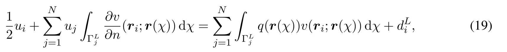
wheredLiis the local defect for thei-th equation.We also have the exact BIE obtained by using the undiscretised exact functionuon the elements,as

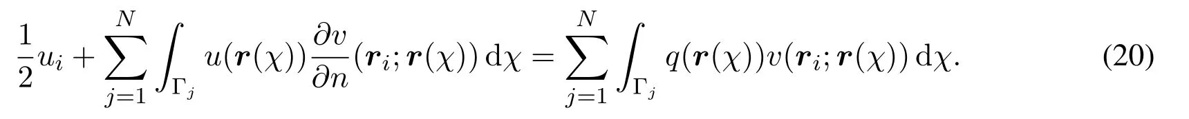
Subtracting Eq.(20)from Eq.(19)gives

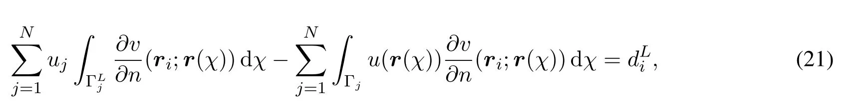
wheredLiis the defect of thei−th equation.If we had this defect,we would add it to the system Eq.(18)and solve to obtain the exact solution at the nodes.The contribution to the defectdLi,from elementj,is given by:

so that the defect for thei−th equation is given by:

The contributions to this defect are significant in the active region,and are assumed negligible elsewhere.However,the exact functionuis not known and we cannot therefore use Eq.(21)to compute the defectdLi.What we can instead do is to formulate and solve a local problem using a fine grid in the active region.The solution to this problem is better than the coarse grid solution because of the fine grid used.At this point,the best solution available is

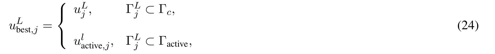
and the best approximations to the integrals in Eq.(22)are

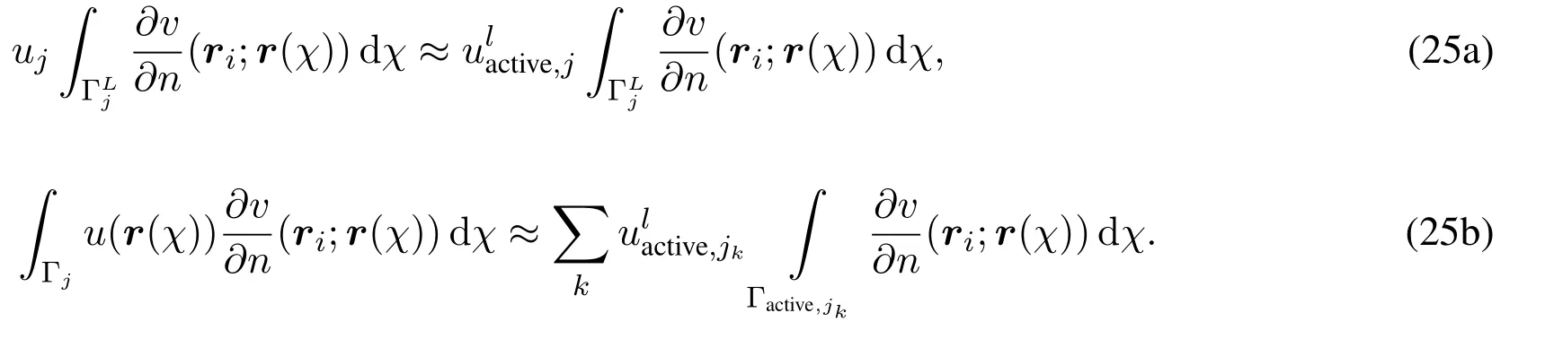
In Eq.(25),we assume that in the local fine grid,a global coarse grid element ΓLjis divided intoKfine elements,k=1,2,...,K,such thatFig.(5)gives an illustration forK=3.

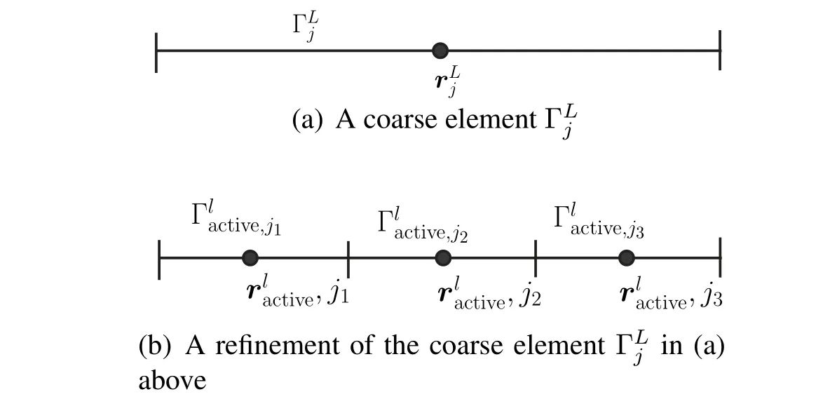
Figure 5:A coarse element that is refined into three elements in the local fine grid,such that [Kakuba and Anthonissen(2014)]

Therefore,using the initial fine grid solution,the initial best approximation of the defect per element is for elements in the active region of the boundary,whereas it is assumed zero for elements outside the active region.We can then compute the defect

The formulation described above can be summarised in matrix form as follows.On the local domain Ωlocalwe have the local fine grid problem

where

The solution ul0active,on the fine grid,which is expected to be more accurate than the coarse grid solution,is then used to approximate the defect for the global coarse grid problem

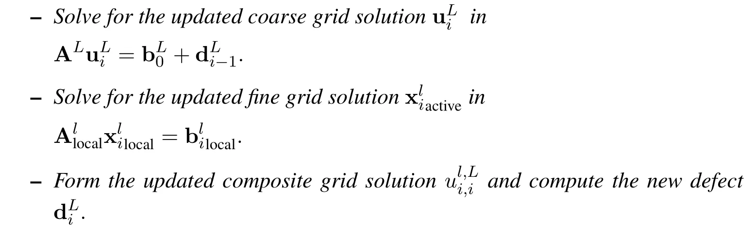
So we solve the updated system

Solving the system in Eq.(31)gives the updated coarse grid solution uL1.At this stage we use the fine grid solution onand the global coarse grid solution to form a composite grid solutionul,Las

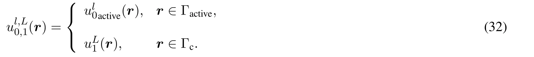
The composite grid solution in Eq.(32) can now be used to compute better boundary conditionson Γinside,and then form and solve the updated fine grid problem

Then we obtain the updated composite grid solution given by:

This step marks the end of one complete cycle of the LDC algorithm.The iteration process is summarised in Algorithm 1,whose more detailed presentation is discussed in Kakuba et al.[Kakuba and Anthonissen(2014)],and results on an example are shown in Fig.6 and Fig.7,where functions are plotted only for the side of the square boundary with the active region.The authors in Kita et al.[Kita and Kamiya (2001)] present a broader review of adaptive error refinement techniques.In this paper,we compare the numerical solution with the exact solution to make conclusions on the error,a kind of error measurement similar to the one attributed to Mullen et al.[Mullen and Rencis(1985)].

Algorithm 3.1.

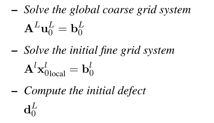
(i)Initialisation

(ii) Fori=1,2,...

4 Properties of the LDC for BEM algorithm as a fixed point iterative scheme

We consider the following Neumann problem

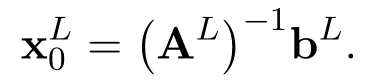
To formulate the LDC algorithm as a fixed point iteration,we need a vector formulation for the steps in Algorithm 3.1.The first step of the algorithm is to solve a global coarse grid problem

for an initial solution xL0.The solution xL0is a vector ofu’s except in one node,the last node,where a Diriclet boundary condition is prescribed to ensure uniqueness of the solution.Using uL0,the boundary conditions and the boundary integral relation Eq.(2)for interior points,we compute the potentialu(r)on Γinside.That is,

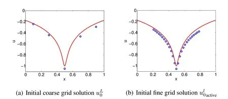
Figure 6:Results of a typical LDC process for a Neumann problem in one iteration (The solid line is the exact solution [Kakuba and Anthonissen(2014)])

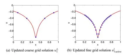
Figure 7:Results of a typical LDC process for a Neumann problem in one iteration (The solid line is the exact solution [Kakuba and Anthonissen(2014)])

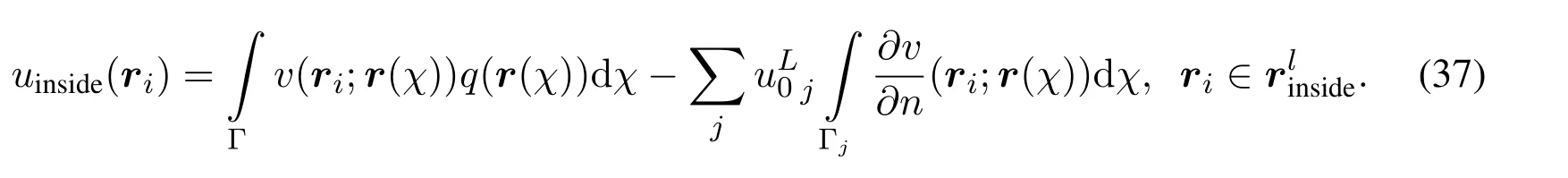
Introducing a vector g and a matrixsuch that

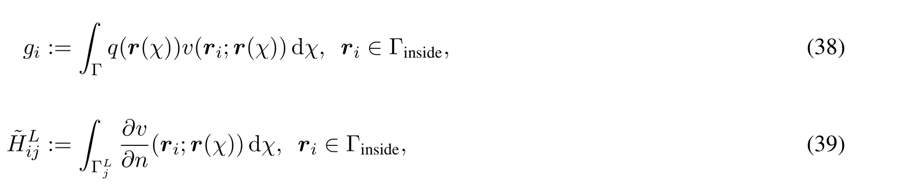
then we can write Eq.(37)as

Using Eq.(40),we obtain Dirichlet boundary conditions on Γinside.The boundary conditions on Γactiveare the same as the given boundary conditions in the global problem since,Γactive⊂Γ.Using(5),we can then write the equations on Γllocalin vector form as

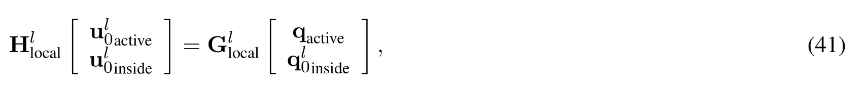
where Hllocaland Gllocalare the BEM H and G matrices on the fine grid of the local problem boundary Γllocal,ulactiveand qlactiveare vectors on the active part Γlactiveof the local problem boundary,and ul0insideand ql0insideare vectors on Γlinside,the part of the local problem boundary that is inside the global domain.The vector ul0insideis known through Eq.(40)and the vector qactiveis known through the boundary conditions.So,we rearrange Eq.(41)as

The matrix Hlactiveis a block of Hlfor which the column index corresponds to nodes in Γlactive.Similarly Hlinsideis a block of Hlfor which the column index corresponds to nodes in Γlinside.The blocks Glactiveand Glinsideare defined analogously.The quantities on the right hand side of Eq.(42)are all known.Let

Then we have

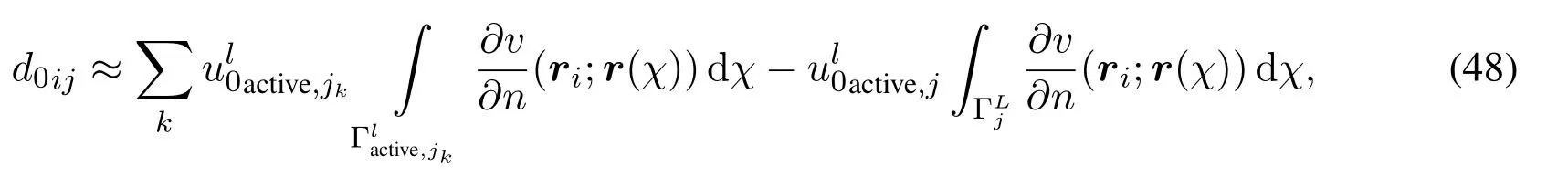
The solution of the system in Eq.(47) gives us another solution ul0activein Γactive,which should be a better approximation ofu(r)than uL0in Γactive,because of the fine grid used.We,then,use this solution to compute the defect and update the global coarse grid solution.The defect on an element ΓLjwhen the collocation node isiis given by:

Since each node communicates with the local active region through integration,the defectd0iis computed for all the nodes.Let us introduce a matrix,defined as

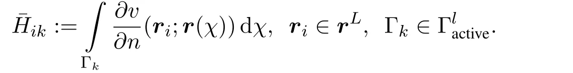
Let PL,lbe a restriction from the fine grid Γlactive,to the coarse grid ΓLactivein Γactive.Then we can write the defect d0as:

At this stage we can assemble a composite grid solution on Γl,Lthat consists of the initial fine grid solution and the updated coarse grid solution.So,

where uL1cis the updated coarse grid solution on Γcoutside the active region Γactive.To complete the updated composite grid solution,we need to solve a new local problem.To this end,we use the solution in Eq.(52) to compute another approximation ofu(r) on Γinside.Thus,we have

andri ∈Γinside.Then we formulate an updated system for the local problem

where

Solving the system in Eq.(55)gives an updated solution ul1activeofu(r)on Γactive.At this stage we have a completely updated composite grid solution given by:

This completes the first iteration that gives us the first updated composite grid solution.The process can be repeated until there is no more change in the solution.In what follows,we formulate the above process as a fixed point iterative process.

Let Ilactivebe an identity of sizeNactive,the number of local elements in Γactive.Then,the part of the local solution in Γactiveis given by,

for thei-th iteration.Consider the updated composite grid solution in Eq.(56)for iterationi+1.Using Eq.(55)and Eq.(57),we have

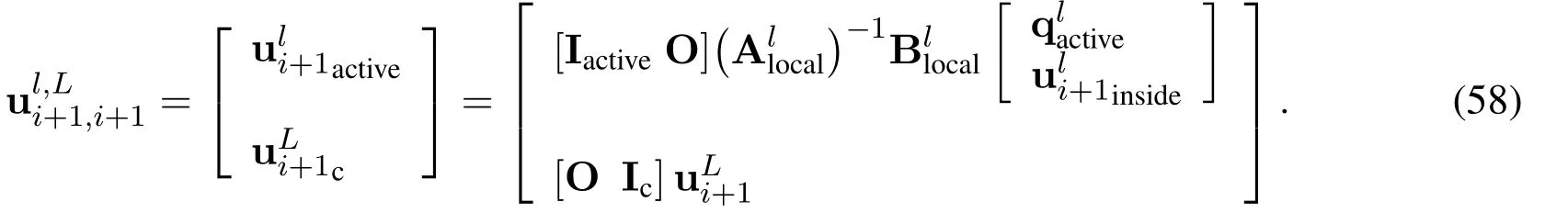
From the second block row of Eq.(58)we have

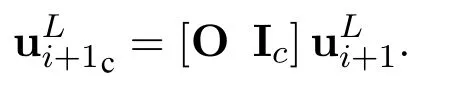
This is the global coarse grid solution outside the active region.For a Neumann problem,we prescribe Dirichlet boundary conditions in the last node,in order to obtain a unique solution.Thus,the last value of the solution vector will be aqvalue.So,in general,we write

Using Eq.(51),we have

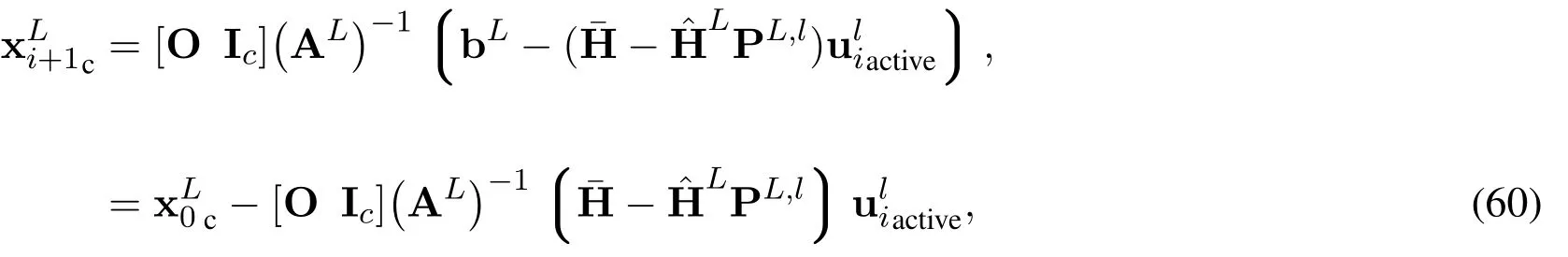
where

Let us consider again Eq.(58).If we introduce a matrix M,defined as

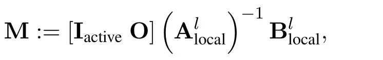
then,from the first block row of Eq.(58),we have

Note that the matrix M is rectangular in size.Let us break it into two blocks,a square block Mactivethat operates on Γlactiveand a block Minsidethat operates on Γlinside.Then we can write Eq.(61)as

From Eq.(53),we see that

Using Eq.(64)in Eq.(62),we have

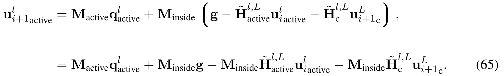
After introducing the following operators

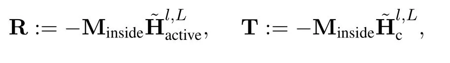
we can then write Eq.(65)as

In Eq.(66) the updated solution on the active grid Γlactiveis expressed in terms of the previous solution and the updated solution outside the active grid.To have an expression for the iteration that takes place on the active region alone,we use Eq.(60) to replace uLi+1,c.Thus,

where bcis the vector of boundary conditions outside the active region.Since the last entry of xLi+1cis aq-value and that of bcis au-value,then matrices D1and D2are the projections

and we have

Introducing the notation

we can write Eq.(69)as

Using Eq.(71)in Eq.(66),we obtain

which can be written as

With a vector v defined as

Eq.(72)can be written as

The vector v remains fixed throughout the iteration,since qlactive,g,bc,remain fixed,andremains the same throughout the iteration.Eq.(73) expresses the iteration that takes place on the fine grid Γlactiveas a fixed point iteration with iteration matrix Q defined as

Thus,we have

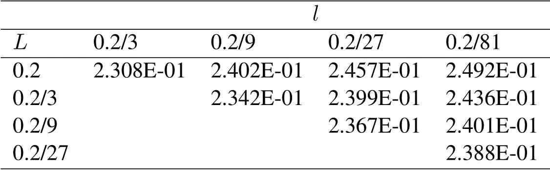
Table 1:Spectral radius of the iteration matrix Q for a Neumann problem for different combinations of fine and coarse grid sizes l and L respectively when local problem domain is the rectangle[0.2, 0.8]×[0, 0.4]and Ω=[0, 1]×[0, 1]

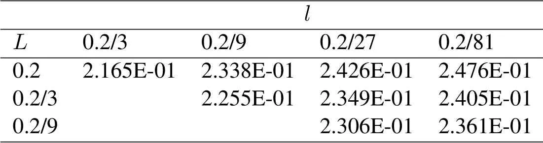
Table 2:Spectral radius of the iteration matrix Q for a Neumann problem for different combinations of grid sizes L and l,and a smaller local problem on[0.4, 0.6]×[0, 0.2]with still Ω=[0, 1]×[0, 1]

This iteration will converge if the spectral radius of the iteration matrix Q is less than unity.In Tab.1 and Tab.2,we have the spectral radii of Q for different combinations ofLandl.All the values are less than unity implying convergence of the fixed point algorithm.

Consider the problem in Eq.(11).We identify Ωlocalas Ωlocal:= [0.2,0.8]×[0,0.4],as illustrated in Fig.2.The LDC is then used with various sizes of coarse grid sizeLand fine grid sizel.We expect the ratios

to be less than unity as well.In Tab.3,we have computed these ratios for five iterations and different combinations of grid sizes.The results fit our expectations,to further illustrate guaranteed convergence of the algorithm.

5 Conclusions

The boundary element method is a relatively new method,whose development started in the late 1970’s although the underlying theory of integral equations could be traced to earlier decades.Its biggest computational disadvantage is that the resulting matrices are full matrices,making the method expensive.In the present study,we have successfully opened a new direction in the implementation of the method,by formulating a fixed point iterative scheme for the LDC technique and showing numerically that the algorithm converges.This approach will be very useful in the implementation of the method in problems withlocalised regions of high activity in the boundary that demand localised regions of high resolution grids.We have shown,by numerical experiments,that the resulting algorithm converges and thus provides a real alternative to composite grid solutions.There is still need to theoretically establish the convergence results,but given the complexity of the matrices involved,this paper presents a good opening to that line of research work.

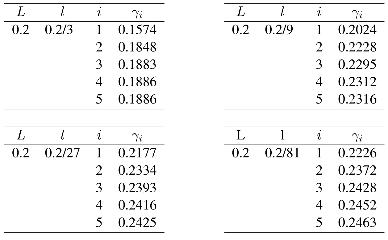
Table 3:The ratios γi defined in Eq.(76)when we use LDC to solve the problem in Eq.(11)

Acknowledgement:We are grateful to the Swedish SIDA-Makerere bilateral project for the funds provided,which enabled time availability for writing this paper.